Vol 7, No 8 (2017)

(1)

Research Article

August

2017

Computer Science and Software Engineering

ISSN: 2277-128X (Volume-7, Issue-8)

Classification of Observations through Combination of the

Dimension Reduction and the Cluster Analysis

Hyeuk Kim*

Division of Global Management Engineering, Hoseo University, Asan, Korea

DOI: 10.23956/ijarcsse/V7I8/01803

Unsupervised learning in machine learning divides data into several groups. The observations in the same group have similar characteristics and the observations in the different groups have the different characteristics. In the paper, we classify data by partitioning around medoids which have some advantages over the k-means clustering. We apply it to baseball players in Korea Baseball League. We also apply the principal component analysis to data and draw the graph using two components for axis. We interpret the meaning of the clustering graphically through the procedure. The combination of the partitioning around medoids and the principal component analysis can be used to any other data and the approach makes us to figure out the characteristics easily.

Keywords— partitioning and around medoids, principal component analysis, unsupervised learning, dimension reduction, baseball

I. INTRODUCTION

Clustering is a main area of data mining and a popular technique for data analysis, used in many fields, including machine learning, bioinformatics, pattern recognition, artificial intelligence, and so on. The most important part of cluster algorithm is how to assign the observations into one of several groups. Observations in the same group have similar characteristics and observations in the different groups have different characteristics as much as possible. Therefore, we can understand complex data easily after assigning them into a few of clusters. We apply the approach to sports data for experiment. Baseball is the most popular sports in Korea of which professional league has started since 1982. The total number of attendance was over 5 million in 2008 and it was over 8 million in the last year. There are several possible outcomes when a batter comes in a plate. We can classify batters based on their styles from various outcomes. The paper is organized as follows. The related papers are explained in the section 2. Section 3 describes data which were used in the paper and section 4 shows the various results of data analysis. We make a conclusion in the final section.

II. LITERATURE REVIEW 2.1. Analysis of sports data

Many researchers have applied the machine learning techniques into sports data. There are two approaches in handling sports data. One approach is to figure out the factors which influence the winning of the game. Lee and Cho [1] suggested the win and loss model through logistic regression model, decision tree model, and neural networks model. Lee and Lee [2] used logistic regression model to predict the outcome of the game and applied the structural equation modelling to investment the effects of factors. Shin, Park, Cho, and Choi [3] tried to find how the individual in a team can affect the result of the single game. They used logistic regression model and decision tree model. Cho, Han, Park, and Heo [4]’s approach was similar to Shim et al.’s approach. However, they focused on the team’s performance to figure out the factors for winning the game. Another approach is to classify players in other sports. The standards of classification can be changed based on the features which are used for analysis. Lutz [5] classified the professional basketball players in United States and explained the effects of the players’ combination. Han, Choen, and Jin [6] analysed the professional basketball players in Korea by clustering and investigated the characteristics of players in each cluster. All papers which are mentioned above handled team sports, but there is also research for an individual game. Choi and Choi [7] classified the golf players by clustering and the generalized canonical correlation biplot.

2.2 Clustering techniques

(2)

ISSN(E): 2277-128X, ISSN(P): 2277-6451, DOI: 10.23956/ijarcsse/V7I8/01803, pp. 30-35

Table I

k-PAM algorithm Procedure

Step Description

1 Choose k initial values among n instances(k<n). The initial points become the centers in each

medoid.

2 Assign all instances into the medoids with the shortest distance by comparing them with the

medoids.

3 Sum the distances between the specific instance and the whole instances inside the same

medoid. Find the instance with the lowest summation of the distance from the previous procedure. It becomes a new center in the corresponding medoid.

4 Return the second step if there is the medoid which has a new center through the third step.

Otherwise stop the clustering procedure.

III. DATA DESCRIPTION

Many statistical measures are developed to evaluate the player’s performance. The area which measures in-game activity in baseball is called Sabermetrics. The examples of the statistical measure in baseball are as follows. RC(Run Created) has been developed by James in 1985 [8]. Furtado [9] has estimated the points by the multiple regression model. The recent popular measures are WAR(Wins Above Replacement), DIPS(Defense Independent Pitching Statistics) for evaluating the pitcher’s own ability, and so on. We only consider the primary data which are available from Korean Baseball League website. There are two reasons not to use the secondary statistics. First, many complex statistical measures are highly correlated since they are derived from the basic statistics. Secondly the purpose of the secondary statistics is to represent the player’s value through one measure. Therefore, it is impossible to distinguish the players with the same value in one integrated measure and the different styles. Korean Baseball Organization offers 32 statistics which are the name, the team, the total number of at-bats, the number of single, the number of double, the number of triple, the number of homerun, bases on balls, hit by pitch, strikeouts, double plays, and so on. We select the variables which are uncorrelated as possible. The unselected statistics are the batting average, on-base percentage, slugging percentage, the success rate of steal, the ratio between bases on balls and strikeout, OPS(on-base plus slugging), batting average with runners in scoring position, and pinch batting average which are generated from other basic statistics. We also ignore the player’s name and the team name since their roles are to identify the record. From the remaining 21 variables, we additionally delete errors, runs batted in, and runs scored which are the measure about defence and the measures influenced on the situation. The last procedure of a variable selection is to remove the variables which are the linear combinations from other eighteen variables. The total plate appearances are the linear combination from at-bats, bases on balls, hit-by-pitch, sacrifice fly, and sacrifice hit. The total bases are the summation of single, two times doubles, three times triples, and four times home runs. Finally, sixteen variables are remained and analysed for research. we classify the baseball players based on the hitting records. Therefore, we do not include the players without the plate appearance even though they join a game as the substitute for run or defense.

IV. DATA ANALYSIS 4.1. Clustering the baseball players

The partitioning around medoids technique is applied to 250 players who have at least one plate appearance in 2013. The selection of the number of clusters is very important issue in clustering. There are many methods to figure out the appropriate number of clusters such as an elbow method, Silhoutte [10], Gap statistic [11], and so on. The suggested numbers of clusters are frequently different based on which methods are applied since they have different algorithms to find the appropriate number of clusters. For example, Silhouette method suggests two clusters and Gap statistic suggests five clusters as the optimal number of clusters. Therefore, it is important for researcher to consider both statistical algorithm and the knowledge about data to decide the number of clusters. It is hard to figure out the characteristics of the clusters if the number of clusters is too small. On the other hand, the representative of each cluster becomes weak if there are too many clusters. We decide to use six clusters to assign players to clusters after considering all aspects of data. The basic results are summarized in Table 2. The players belonging to Cluster ID 5 and Cluster ID 6 are named as Borderline Player and Second-Stringer, respectively since their numbers of plate appearance are little. The players in the fifth cluster take average 112.1 plate appearances in 2013 season and the players in the sixth cluster take average 17.5 plate appearances in 2012 season. We make a conclusion that the players in both clusters are temporarily in the first string.

Table III

Description of Players in Each Cluster in 2013

Cluster ID Type Number of Players Number of Players(%)

1 Powerful Starter 13 5

2 Ordinary Starter 23 9

3 Speedy Starter 14 6

4 Substitute 47 19

5 Borderline Player 57 23

(3)

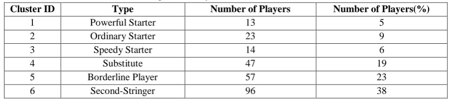
We apply the principal component analysis to 250 players to visualize the relationship among the clusters. The first and the second components are used as x-axis and y-axis, respectively.

Fig. 1 Clustering of baseball players in 2013 when the number of clusters is six

We can figure out which cluster belongs to a certain circle in Figure 1 if we consider the direction of vectorized variables. The circle located on the upper left corner denotes powerful starters, the circle located on the lower left corner denotes speedy starters. Four circles in the middle of Figure 1 describes ordinary starters, substitutes, borderline players, and second-stringers from left to right. The averages of 16 variables in each cluster by PAM algorithm are described in Table 3 and 4.

Table IIIII

Averages of Variables of Players in 2013 in Each Cluster (1)

ID Type G PA 1B 2B 3B HR SB CS

1 Powerful Starter 119.3 502.5 106.1 20.7 0.3 20.3 6.0 3.3

2 Ordinary Starter 113.9 450.0 85.1 21.6 2.1 8.3 12.5 5.2

3 Speedy Starter 115.0 419.5 75.5 15.7 5.1 3.9 24.8 8.7

4 Substitute 93.0 299.4 48.0 12.2 1.0 4.6 5.0 2.6

5 Borderline

Player

56.6 112.1 17.8 4.2 0.3 0.9 3.1 1.4

6 Second-Stringer 11.7 17.5 2.3 0.5 0.1 0.2 0.4 0.2

G: Games played, PA: Plate Appearance, 1B: Single, 2B: Doubles, 3B: Triples, HR: Home Runs, SB: Stolen Bases, CS: Caught Stealing

Table IV

ID Type SAC SF BB IBB HBP SO GDIP MH

3 Speedy Starter 10.6 3.2 39.9 0.6 7.6 66.1 5.6 24.9

4 Substitute 6.3 2.4 27.5 0.4 5.2 52.9 6.0 15.4

5 Borderline

Player

2.4 0.7 10.4 0.1 1.5 21.8 2.5 4.6

6 Second-Stringer 0.2 0.1 1.2 0.0 0.2 4.9 0.4 0.4

SAC: Sacrifice Bunts, SF: Sacrifice Flies, BB: Bases on Balls, IBB: Intentional Walks, HBP: Hit by Pitch, SO: Strikeouts, GDIP: Ground into Double Plays, MH: Multiple Hits

(4)

Table V

ID Type AVG OBP SLG OPS BB/K P/H RBI R

3 Speedy Starter 0.279 0.361 0.385 0.746 0.644 0.247 38.3 60.4

4 Substitute 0.257 0.339 0.367 0.706 0.603 0.274 31.0 32.9

5 Borderline

Player

0.234 0.315 0.304 0.619 0.530 0.221 10.2 12.5

6 Second-Stringer 0.160 0.212 0.208 0.420 0.197 0.133 1.3 2.0

AVG: Batting Average, OBP: On-base Percentage, SLG: Slugging Percentage, OPS: On-base Plus Slugging Percentage, BB/K: the ratio between bases on balls and strikeouts, P/H: the ratio between the number of hits excluding singles and the number of hits, RBI: Runs Batted In, R: Runs Scored

We apply the same approach to the players’ record in 2012 to verify whether it is robust to assign players into 6 clusters or not. The league structures in 2012 and 2013 are different since a new team joined Korean Baseball League. We compare the league structure in 2012 with the league structure in 2013 in Table 6.

Table VI

Comparison of League Structures between 2012 and 2013

2012 2013

total games 133 128

number of teams 8 9

games between two teams 19 16

number of eligible players 226 250

number of eligible players per team 28.3 27.8

runs per game 4.12 4.65

The number of eligible players is reduced from 250 in 2013 to 226 in 2012 since the number of teams is 8 in 2012 compared with 9 in 2013. We find that there is no difference in two years when we investigate the number of eligible players per team in 2012 and 2013. We follow the same research procedure for the players’ data in 2012 and generate the tables like Table 2 to 5.

Table VII

Description of Players in 2012 in Each Cluster

Cluster ID Type Number of Players Number of Players(%)

1 Powerful Starter 5 2

2 Ordinary Starter 29 13

3 Speedy Starter 15 7

4 Substitute 44 19

5 Borderline Player 46 20

6 Second-Stringer 87 37

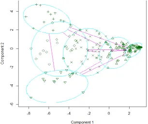
The shapes of clusters are plotted on the two-dimensional graph of which x-axis is the first component and y-axis is the second component from the result of the principal component analysis. They are described on the graph in Figure 2.

(5)

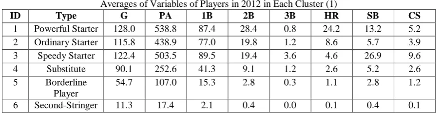
Table VIVII

ID Type G PA 1B 2B 3B HR SB CS

3 Speedy Starter 122.4 503.5 89.5 19.4 3.6 4.6 26.9 9.6

4 Substitute 90.1 252.6 41.3 9.1 1.2 2.6 5.2 2.6

5 Borderline

Player

54.7 107.0 15.3 2.8 0.3 1.1 2.8 1.2

6 Second-Stringer 11.3 17.4 2.1 0.4 0.0 0.1 0.4 0.1

G: Games played, PA: Plate Appearance, 1B: Single, 2B: Doubles, 3B: Triples, HR: Home Runs, SB: Stolen Bases, CS: Caught Stealing

Table IX

ID Type SAC SF BB IBB HBP SO GDIP MH

3 Speedy Starter 11.9 4.4 41.9 1.1 6.0 61.4 7.3 30.4

4 Substitute 6.9 1.8 21.0 0.4 3.0 44.1 4.9 12.1

5 Borderline

Player

3.2 0.6 8.3 0.2 1.1 22.4 1.8 3.2

6 Second-Stringer 0.2 0.1 1.2 0.0 0.3 4.4 0.3 0.3

SAC: Sacrifice Bunts, SF: Sacrifice Flies, BB: Bases on Balls, IBB: Intentional Walks, HBP: Hit by Pitch, SO: Strikeouts, GDIP: Ground into Double Plays, MH: Multiple Hits

Table X

ID Type AVG OBP SLG OPS BB/K P/H RBI R

3 Speedy Starter 0.266 0.336 0.357 0.693 0.797 0.234 44.3 62.2

4 Substitute 0.246 0.319 0.333 0.652 0.518 0.240 23.0 24.5

5 Borderline

Player

0.203 0.278 0.266 0.544 0.417 0.198 8.1 10.8

6 Second-Stringer 0.142 0.197 0.180 0.376 0.189 0.132 1.1 1.5

AVG: Batting Average, OBP: On-base Percentage, SLG: Slugging Percentage, OPS: On-base Plus Slugging Percentage, BB/K: the ratio between bases on balls and strikeouts, P/H: the ratio between the number of hits excluding singles and the number of hits, RBI: Runs Batted In, R: Runs Scored

When we compare the player’s record in 2012 with the players’ record in 2013, we find that the compositions in both years are same. We can figure out the characteristics of players in each cluster from the ratio statistics in Table 5 and 10.

V. CONCLUSIONS

Clustering is the tasking of grouping objects in such a way that objects in the same group are similar as much as possible and objects in the different groups are different as much as possible. We categorize data into several clusters and figure out the characteristic of data in each cluster. In the research, we use data about the professional baseball players in Korea to classify them. The partitioning around medoids technique is applied to the players who have at least one plate appearance. Then the generated clusters are plotted on the graph with the first component and the second component as the x-axis and the y-axis from the principal component analysis. Through clustering, we define 6 clusters and each cluster has its unique characteristic. We apply the same approach to the players in another year to get the robust result. Observations with the various features can be categorized based on their characteristics and the approach applied in the research makes us enlarge the understanding of data.

REFERENCES

[1] J. T. Lee and H.-S. Cho, “An analysis on the home-field advantage in Korean pro-baseball with logistic

regression model,” Journal of the Korean Data and Information Science Society, 21(6), pp. 1041-1049, 2009.

[2] H.-Y. Lee and S.-K. Lee, “Relation analysis between victory and the records of Korean professional baseball,”

(6)

[3] S.-K. Shin, K.-C. Park, Y.-S. Cho, and S.-H. Choi, “A study on analyzing factors affecting the outcome of

Korean professional baseball games: A case of Samsung Lions,” Journal of the Korean Data Analysis Society,

9(4), pp. 2071-2083, 2007.

[4] Y.-S. Cho, J.-T. Han, C. Park, and T.-Y. Heo, “A statistical analysis of professional baseball team data: The case

of the Lotte Giants,” The Korean Journal of Applied Statistics, 23(6), pp. 1191-1199, 2010.

[5] D. Lutz, “A cluster analysis of NBA players,” in Proceedings in MIT Sloan Sports Analytics Conference, 2012.

[6] S. Han, S. Cheon, and S. Jin, “Clustering Korean professional basketball players by using k-medoids

clustering,” Journal of the Korean Data Analysis Society, 10(6B), pp. 3423-3433, 2008.

[7] T.-H. Choi and Y.-S. Choi, “A study on the relationship between skill and competition score factors of KLPGA

players using canonical correlation biplot and cluster analysis,” The Korean Journal of Applied Statistics, 21(3), pp. 429-439, 2008.

[8] B. James, The Bill James historical baseball abstract, Villard, 1985.

[9] J. Furtado, The 1999 big bad baseball annual: The book baseball deserves, Maters Press, 1999.

[10] P. J. Rousseeuw, “Silhouette: A graphical aid to the interpretation and validation of cluster analysis,”

Computational and Applied Mathematics, 20, pp. 53-65, 1987.

[11] R. Tibshirani, G. Walther, and T. Hastie, “Estimating the number of clusters in a data set via the gap statistic,”