Volume 30 (2010)
International Colloquium on Graph and Model
Transformation On the occasion of the 65th birthday of
Hartmut Ehrig
(GraMoT 2010)
Stepping from Graph Transformation Units to Model Transformation
Units
Hans-J¨org Kreowski, Sabine Kuske, Caroline von Totth
24 pages
Guest Editors: Claudia Ermel, Hartmut Ehrig, Fernando Orejas, Gabriele Taentzer Managing Editors: Tiziana Margaria, Julia Padberg, Gabriele Taentzer
Stepping from Graph Transformation Units to Model
Transformation Units
Hans-J¨org Kreowski1, Sabine Kuske2, Caroline von Totth3∗
1[email protected] 2[email protected]
Department of Computer Science University of Bremen, Germany
Abstract:Graph transformation units are rule-based entities that allow to transform source graphs into target graphs via sets of graph transformation rules according to a control condition. The graphs and rules are taken from an underlying graph transformation approach. Graph transformation units specify model transforma-tions whenever the transformed graphs represent models. This paper is based on the observation that in general models are not always suitably represented as sin-gle graphs, but they may be specified as the composition of a variety of different formal structures such as sets, tuples, graphs, etc., which should be transformed by compositions of different types of rules and operations instead of single graph transformation rules. Consequently, in this paper, graph transformation units are generalized to model transformation units that allow to transform such kind of com-posed models in a rule-based and controlled way. Moreover, two compositions of model transformation units are presented.
Keywords:graph transformation, model transformation, transformation units, mo-del transformation units
1
Introduction
Computers are devices that can be used to solve all kinds of data-processing problems – at least in principle. The problems to be solved come from economy, production, administration, science, education, entertainment, and many other areas. There is quite a gap between the problems as one has to face them in reality and the solutions one has to provide so that they run on a computer. Therefore, computerization is concerned with bridging this gap by transforming a problem into a solution. Many efforts in computer science contribute to this need for transformation. First of all, compilers are devices that transform programs in a high-level language into programs in a low-level language where the latter are nearer and more adapted to the computer than the former. The possibility and success of compilers have fed the dream of transforming descriptions of data-processing problems automatically or at least systematically into solutions that are given by
∗ The authors would like to acknowledge that their research is partially supported by the Collaborative Research
smoothly running programs. In recent years, the term model transformation has become popular for this idea.
In this paper, graph transformation units are generalized to model transformation units as rule-based devices for modeling model transformations in a compositional framework. Our approach has three sources of inspiration:
1. Following the ideas of model-driven architecture (MDA; cf., e.g., [Fra03]), the aim of model transformation is to transform platform-independent models (PIMs), which allow to describe problems adequately, into platform-specific models (PSMs), which run properly and smoothly on a computer. As a typical description of the PIMs one may use UML diagrams, while PSMs are often just programs in some common higher-level language like Java or C++. A significant model transformation language within the framework of MDA is the QVT standard of the OMG [OMG08].
2. One encounters quite an amazing number of model transformations in theoretical com-puter science – in formal language theory as well as in automata theory in particular. These areas provide a wealth of transformations between various types of grammars and automata like, for example, the transformation of nondeterministic finite automata into de-terministic ones, or of pushdown automata into context-free grammars (or the other way round), or of arbitrary Chomsky grammars into the Pentonen normal form (to give a less known example).
3. Graph transformation units (cf., e.g., [KKS97, KK99, KKR08]) are rule-based devices to model binary relations between initial and terminal graphs. If the initial graphs are interpreted as input models and the terminal graphs as output models, then such a unit embodies a model transformation. The transformation of UML sequence diagrams into UML collaboration diagrams in [CHK04] and the transformation of well-structured flow diagrams intowhile-programs in [KHK06] are examples of this kind. This observation supports the idea to use graph transformation units as building blocks for the modeling of model transformations.
2
Preliminaries
In this section, we recall the notion of a graph rule base providing a class of graphs, a class of rules and a rule application operator. In the following sections graphs are used as basic visual models and rules are used for their elementary transformations. Besides graphs, we use iden-tifiers, truth values, and non-negative integers as smallest atomic models. Moreover, cartesian products, free monoids, and powersets are recalled because these constructions will be used to build up composite models in the next section.
2.1 Graph Rule Bases
Agraph rule base B= (G,R,=⇒)consists of a class of graphs G, a class of rules R, and a
rule application operator=⇒with=⇒ r ⊆
G×G for everyr∈R. The rule application operator
is used in infix notation, i.e,(G,H)∈=⇒
r is denoted byG=⇒r H. Subsections2.2through 2.4 present examples for the components of rule bases which are used throughout this paper.
2.2 Graph Classes
There are many different kinds of graph classes, two of which are explored here further: the class of directed edge-labeled graphs and the class of finite state graphs, the latter being a subclass of the former.
Directed edge-labeled graphs. The class of directed, edge-labeled graphs with individual, possibly multiple edges is defined as follows. Let Σbe a set of labels. A graphover Σis a
systemG= (V,E,s,t,l)whereV is a set ofnodes,Eis a set ofedges,s,t:E→V are mappings assigning asource s(e)and atarget t(e)to every edge inE, andl:E→Σis a mapping assigning
a label to every edge inE. An edgeewiths(e) =t(e)is also called aloop. For a nodev∈V the number of edges which havevas source is denoted byoutdegree(v)and the number of edges that point tovis theindegreeofv. An edgeewith labelxis called anx-pointer ifindegree(s(e)) =0 andoutdegree(s(e)) =1. The componentsV,E,s,t, andlofGare also denoted byVG,EG,sG,
tG, andlG, respectively. The set of all graphs overΣis denoted byGΣ.
For graphsG,H∈GΣ, agraph morphism g:G→His a pair of mappings gV:VG→VH and
gE:EG→EHthat are structure-preserving, i.e.,gV(sG(e)) =sH(gE(e)),gV(tG(e)) =tH(gE(e)), andlH(gE(e)) =lG(e)for alle∈EG.
If the mappingsgV andgEare inclusions, thenGis called asubgraphofH,denoted byG⊆H. For a graph morphismg: G→H, the image ofGinHis called amatchofGinH, i.e., the match ofGwith respect to the morphismgis the subgraphg(G)⊆H.
Finite state graphs. Two particular subclasses ofGΣare the classes of finite state graphs and
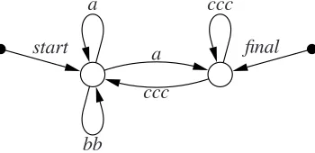
finite state graphs with word transitions respectively. More concretely, letIbe some input alpha-bet such thatI∗⊎ {start,final} ⊆Σ1. Then the graph inFigure 1represents a finite state graph with word transitions overI={a,b,c}, where the edges labeled withw∈I∗represent transitions,
start a final
ccc a
bb
ccc
Figure 1: A finite state graph with word transitions
start
final a
b b
c c
c
c c c
a
Figure 2: A finite state graph
and the sources and targets of the transitions represent states. The start state is indicated with a start-pointer and every final state with afinal-pointer. States are depicted as unfilled circles whereas all other nodes are shown as small filled circles. Figure 2 shows a finite state graph where each transition is labeled with a symbol fromI.
2.3 Rules
To be able to transform graphs, rules are applied to the graphs yielding graphs again. One rule class that can be used to transform graphs inGΣ is defined as follows. Arule r= (L⊇K⊆R)
consists of three graphsL,K,R∈GΣ such thatKis a subgraph ofLandR. The componentsL,
K, andRofrare calledleft-hand side, gluing graph, andright-hand side, respectively. A rule may be depicted asL→RifKis clear from the context (the numbered nodes form the common gluing graph).
An example of a rule is given inFigure 3. The left-hand side of this rule consists of two nodes
refine: 1 2
xyu
1 2
x yu
−→ x,y∈I u∈I∗
1 and 2 and an edge from node 1 to node 2 that is labeled with a wordxyufrom some alphabet
I∗ wherex and y are symbols ofI. The gluing graph consists of the two nodes 1 and 2; the right-hand side is obtained from the gluing graph by inserting a new nodevand two new edges
e1ande2wheree1points from node 1 tovand is labeled withx, ande2points fromvto node 2 and is labeled withyu.
2.4 Rule Application
The application of a graph transformation rule to a graphGconsists of replacing a match of the left-hand side inGby the right-hand side in such a way that the match of the gluing graph is kept. Hence, the application ofr= (L⊇K⊆R)to a graphG= (V,E,s,t,l)consists of the following three steps.
1. A matchg(L)ofLinGis chosen.
2. Now the nodes ofgV(VL−VK)are removed, and the edges ofgE(EL−EK)as well as the edges incident to removed nodes are removed yielding theintermediate graph Z⊆G.
3. Afterwards the right-hand side Ris added to Z by gluing Z withR ing(K) yielding the graphH=Z⊎(R−K)withVH=VZ⊎(VR−VK)andEH=EZ⊎(ER−EK). The edges of
Z keep their labels, sources, and targets so thatZ⊆H.The edges ofRkeep their labels; they also keep their sources and targets provided that those belong toVR−VK.Otherwise,
sH(e) =g(sR(e))fore∈ER−EK withsR(e)∈VK,andtH(e) =g(tR(e))fore∈ER−EK withtR(e)∈VK.
The application of a ruler to a graphGis denoted byG=⇒
r H, whereH is the graph resulting from the application ofrtoG. A rule application is called adirect derivation.
If the rulerefineinFigure 3is applied to a finite state graph, it splits a word transition labeled with a wordwof length at least two into two consecutive transitions, the first of which takes the first symbol ofw, while the second one gets labeled with the remainder of w. In particular, if
refineis applied as long as possible to the finite state graph inFigure 1, one gets the finite state graph inFigure 2.
2.5 Further Basic Types
In addition to graph rule bases, we assume a set of identifiersID, the set of truth values BOOL= {TRUE,FALSE}, and the set of non-negative numbersN. All these sets are equipped with the
usual predicates and operations, i.e. the arithmetic operations like+,−,·,≤,=,etc. for N, the
Boolean operations like∧,∨,¬,→,etc. for BOOL, and the equality predicate=forID. All involved sets may be subject to the following three constructions that yield sets again:
1. the cartesian productX1× · · · ×Xkfor setsX1, . . . ,Xk,k∈N;
2. the free monoidX∗for a setX;
Furthermore we assume that the usual operations of these data types are available, like the projections in the case of the product, concatenation and other string-processing operations in the case ofX∗and the usual operations and predicates on sets like∪,∩,∈,⊆,etc.
3
Models and Model Types
Many models used in computer science are of a graphical, diagrammatic, and visual nature, and they can be represented as graphs in an adequate way in most cases. Moreover, further types of elementary models such as numbers, truth values, or identifiers may be useful in addition to graphs. And models may not occur only as singular items, but also as tuples or as some other collections of models like sequences and sets. To cover this, we define models and their types in a recursive way.
Definition 1(models and their types) Models together with their types are recursively defined as follows:
1. LetY be a class of graphsG,ID, BOOL, orN. Then eachy∈Y is amodel of type Y.
2. Ifmiis a model of typeTifori=1, . . . ,kfor somek∈N, then thek-tuple(m1, . . . ,mk)is amodel of type T1× · · · ×Tk.
3. Ifmiis a model of typeT fori=1, . . . ,kfor somek∈N, then the sequencem1· · ·mkis a
model of type T∗.
4. Ifmis a set of models of typeT, thenmis amodel of type set(T).
Note that in this way every model gets a type which is a set of models, but can serve as a name on the syntactic level as well. To stress the semantic level we may writeM(T)forT.
Point 1 makes sure that all graphs and – in this way – all diagrams with graph representations are models. Besides graphs, truth values, numbers and identifiers become available as elementary models. Point 2 allows one to consider a k−tuple of models as a model and makesk models simultaneously available in this way. Point 3 and Point 4 also make many models of the same type available at the same time. While Point 3 provides them as a sequence, Point 4 collects them as a set.
The types of models as introduced above may be considered as free because they are based on the free constructions product, free monoid, and power set. But in many cases, it may not be reasonable to transform all models of a free type without any further restriction. For example, a Chomsky grammarG= (N,T,P,S)is not just a quadruple of typeset(ID)×set(ID)×set(ID∗×
Definition 2(constrained model types) LetT be a model type.
1. ThenX(T)is a class ofconstraintsif eachx∈X(T)specifies a set of models of typeT,
i.e.SEM(x)⊆M(T).
2. Forx∈X(T),hT with xiis called aconstrained model type. The models of this type are
the models ofSEM(x), denoted byM(hT with xi).
The definition is used in a recursive way considering the free model types and the con-strained model types both as model types. Consequently, one can build types of the form hhT with xiwith yiwith iterated constraints.
3.1 Examples for Constraints
1. For the model typeG, constraintsxwithSEM(x)⊆G are called graph class expressions
in the framework of graph transformation units and are extensively used there to specify initial and terminal graphs. Examples of graph class expressions are the following.
(a) Single graphsZ∈G withSEM(Z) ={Z}are useful as start graphs of graph
gram-mars.
(b) ForG =GΣ withΣ⊆ID, a subsetX⊆ΣdescribesSEM(X) =GX and may serve as
terminal labels.
(c) ForG =GΣandX⊆Σ, the expressionpointers(X)specifies all graphs inGΣin which
all edges labeled with somex∈X are pointers (cf.Subsection 2.2).
(d) ForG =GΣ and X⊆Σ, the expression one(X)specifies all graphs Gin which for
eachx∈X there occurs exactly onex-labeled edge, i.e.,|{e∈EG|lG(e) =x}|=1 for eachx∈X.
2. Logical formulas are further typical examples for constraints. They may involve model variables and the usual predicates and operations of the basic and free types:
(a) Boolean operations in case of BOOL like¬,∧,∨,→;
(b) arithmetic operations and predicates onNlike+,·, mod, =,≤;
(c) string operations and predicates onX∗for some setX, like concatenation, transposi-tion, equality;
(d) set operations and predicates like∪,∩,⊎, =,⊆,∈.
Consider, for example, a model (x,y,X,Y,m,n,u,v,G,H) of type ID×ID×set(ID)×
set(ID)×N×N×ID∗×ID∗×GΣ×GΣ. Then one may add the following constraints:
x=y,x∈X,y∈Y,X∩Y =/0,m≤n,length(u)≥n,uv6=vu,u=vtranspos(v),G⊆H,
G∈GX, wherelengthmeasures the length of a worduand returns an integer, andtranspos
3. Another frequently used constraint for graphs and sets is the requirement of finiteness indicated by the constant model class expressionfiniteness. Instead ofhGΣwith finitenessi
we may writefin(GΣ), andfinset(ID)instead ofhset(ID)with finitenessi.
3.2 Examples for Constrained Model Types
1. Finite state automata with word transitions can be defined as a constrained model type, i.e. afinite state automaton fsa= (I,G)is a pair of type hset(ID)×GΣwith(∆⊆Σ)∧(G∈
(∆∩pointers({start,final})∩one({start})))iwhere∆=I∗⊎ {start,final}. The constraint
means that every state graphGis labelled overI∗⊎ {start,final},final- andstart-edges are pointers, and there is exactly one start-pointer. In the following, the constrained model type of finite state automata with word transitions is denoted byFSA∗. The type of finite state automata the transitions of which are labelled only with single symbols fromI, can be defined as the finite state automata inFSA∗, but where in the constraint I∗is replaced byI, i.e.,∆=I⊎ {start,final}. The type of all finite state automata with single-symbol
transitions is denoted byFSA.
2. Chomsky grammars can be introduced in the framework above as models nearly in the same way as they are defined in the literature.
AChomsky grammar G= (N,T,P,S)is a quadruple of typeset(ID)×set(ID)×set(ID∗×
ID∗)×ID withfiniteN,T andP,N∩T= /0,S∈N, and(u,v)∈Pimpliesu,v∈(N∪T)∗ andu∈/T∗.Gisright-linearif, in addition,(u,v)∈Pimpliesu∈Nandv∈(T+N)∪ {ε}
whereε denotes the empty string.
More formally, the constraint of an arbitrary Chomsky grammar is with N,T,P∈finset(ID) ∧N∩T =/0∧S∈N∧((u,v)∈P→(u,v∈(N∪T)∗∧u6∈T∗)). And in case of right-linear grammars one must add((u,v)∈P→(u∈N∧v∈T+N∪ {ε})). The type of right-linear
grammars will be denoted byRLG. For explicit use below we mention here also the type
RLG×GΣ which will be used for transforming right-linear grammars into finite state
au-tomata.
4
Actions and Model Transformation Processes
In this section, the dynamic part of model transformations is introduced. The basic notion is that of an action that describes an elementary step of model transformations. Then the iteration of such steps provides more complex transformations.
It is worth noting that in this paper we do not explicitly consider infinite model transformations because the purpose of model transformation units is to convert input models into output models in finitely many steps. Infinite processes are considered in [HKK09].
Each modelmcan be identified with the 1-tuple(m)so that one may consider tuples of models only without loss of generality. Given such a tuple (m1, . . . ,mk), an action is also a k-tuple
is a number, string or set, then ai may operate on it yielding a modified number, string or set respectively. Moreover, we employ the void actionai=−meaning thatmiremains unchanged. If the component actions are performed, then a new tuple(m′1, . . . ,m′k) of models is obtained. This is made precise in the following definition.
Definition 3(actions) LetT1× · · · ×Tkbe a model type.
1. Then anaction a= (a1, . . . ,ak) is a k-tuple such that one of the following holds for i= 1, . . . ,k:
(a) ai=−,
(b) ai∈Rprovided thatTi⊆G,
(c) ai=renameprovided thatTi⊆IDwhererenameis some mapping onTi,
(d) aiis a term of operations with a distinguished variable of typeNand which evaluates toNprovided thatTi=N.
(e) the same as (d) replacingNby BOOL,T∗andset(T)for some typeT,
(f) recursively, ai is an action provided that Ti is a product type with more than one component.
2. Letm= (m1, . . . ,mk)∈M(T1× · · · ×Tk). Then the action(a1, . . . ,ak)may be performed onmyieldingm′= (m′1, . . . ,m′k)∈M(T1× · · · ×Tk)denoted bym=⇒
a m
′ if the following
holds fori=1, . . . ,k:
(a) m′i=mi ifai=−; (b) mi=⇒
ai m ′
iifai∈R;
(c) m′i=ai(mi)ifai=renameorai is a term as described in 1.(d) or (e). (d) mi=⇒
ai m ′
iifaiis an action.
3. LetAbe a set of actions. Then amodel transformation processis a sequence of performed actionsm=m0=⇒
a1
m1=⇒
a2
· · ·=⇒
an mn=m
′with theaction sequence a
1· · ·an∈A∗. Such a process may be denoted bym=n⇒
A m
′orm=∗⇒ A m
′if the omitted details do not matter. The
set of model transformation processes overAis denoted byMTP(A).
4.1 Examples for Actions
Let(N,T,P,S,G)be an arbitrary model of typeRLG×GΣas defined in point 2 ofSubsection 3.2.
1. An action that removes a nonterminal symbol X from the first component of the right-linear grammar(N,T,P,S)and then inserts a state labeled withXin the graph component can be defined as(remove(X),−,−,−,node(X)), whereremove(X)removesXfromN(if
node(X): /0
X
−→
Figure 4: Graph transformation rulenode(X)
edge(X,u,Y): 1 2
X Y
1 2
X u Y
−→
Figure 5: Graph transformation ruleedge(X,u,Y)
2. An action that removes a rule with a non-empty right-hand side from the right-linear gram-mar while inserting a corresponding transition in the graph that contains a state for every nonterminal of the rule can be defined as (−,−,remove((X,uY)),−,edge(X,u,Y)); the graph transformation ruleedge(X,u,Y)is given inFigure 5.
Model transformation processes are nondeterministic in three respects. First, the rule applica-tions in graph model components are nondeterministic as some rules may be applicable at several matches. Second, although the operations of the basic types are functional, the evaluations of the action terms of these types may not lead to unique values as the terms can contain free variables with a variety of instantiations. Third, there may be a choice of many actions that can process a current model, and the only regulating requirement for actions is that of sequential composition, which is that one action is executed after the other. Sometimes such nondeterminism is desired, convenient, or unavoidable. But in other cases one would like to avoid nondeterminism, or cut it down at least. This can be achieved by choosing rules and actions in such a way that only one or a few of them can be applied and performed. But the rules and actions may become quite complicated. Another possibility is extra regulation which can be provided by control conditions.
Definition 4(control conditions) LetAbe a set of actions. ThenC is a class ofcontrol condi-tionsifSEM(c)⊆MTP(A)for everyc∈C.
4.2 Examples for Control Conditions
In the area of graph transformation, control conditions are frequently expressions over rules. Many of these kinds of control conditions can be generalized by replacing rules with actions.
1. A typical kind of control conditions are regular expressions overA. Each regular expres-sionrspecifies a regular languageL(r). A model transformation processm=∗⇒
A m
′belongs
toSEM(r)if and only if its action sequence belongs toL(r). In the following, the operators concatenation, union, and Kleene star on languages will be denoted on the level of regular expressions as a semicolon, a vertical bar and a star, respectively.
model transformation process belongs toSEM(≤) if and only if each performed action
mi−1=⇒
ai mihas highest priority meaning that there is nomi−1=⇒a mwitha≥aibutai6≥a. 3. For any action a, the control conditiona! requires to applyaas long as possible. Hence,
m=∗⇒ A m
′ is inSEM(a!)if the application sequence is in{a}∗and there is nom′′such that
m′=⇒ a m
′′. (Due to the fact that model transformation processes are finite, this means that
SEM(a!) = /0 ifacan be applied infinitely often to any model m.) This condition can be combined with regular expressions in a straightforward way. For example, the expression
a1!;a2! requires to apply firsta1as long as possible and thena2as long as possible.
5
Model Transformation Units
The previous sections provide all the ingredients that are needed to introduce model transforma-tion units as devices to specify model transformatransforma-tions. Such a unit consists of the type of models to be transformed, of the actions to be performed, and of the control condition that regulates the transformation process. Moreover, the types of input and output models are specified, including their relation to the type of working models. The reasons to separate input, output and working models is that input and output may have different types and that it may be convenient to use further component models for intermediate processing.
In other words, an input modelmof typehI1× · · · ×Ikwith xi(i.e. a model of typeI1× · · · ×Ik that satisfies the constraintx) is first of all extended to a working modelmof typeT1× · · · ×Tlby taking the components ofmas components ofmaccording to a mappinginitial. This mapping yields for each component ofmthe positions inm(i.e. the numbers out of 1, . . . ,l) where the component should be used. Clearly, each position inmmay be associated in this way with with at most one component of the input type. The components of the working model not covered byinitialare initialized by the initial models of the respective component types. Initial models are chosen in some appropriate way, like 0 forTj =N, etc. Thenmis transformed intom′ by performing the given actions such that the control condition is satisfied. Afterwards an output modelm′ of typehO1× · · · ×Onwith yiis constructed according to a mapping terminal. This mapping selects for every position inm′ (i.e. for every number out of 1, . . . ,n) a component of
m′. Moreover, it must be assured that the obtained modelm′satisfies the constrainty.
Definition 5(model transformation unit)
1. Amodel transformation unitis a systemmtu= (ITD,OTD,WT,A,C)where
− WTis a product typeT1× · · · ×Tl calledworking type,
− ITDis theinput type declarationwhich consists of the constrained product typehI1×
· · · ×Ikwith xiand a mappinginitial:[k]→set[l]such thatinitial(i)∩initial(j) =/0 fori6= jandIi=Tjfori=1, . . . ,kand j∈initial(i),
− OTD is the output type declaration which consists of a constrained product type hO1×· · ·×Onwith yiand an injective mappingterminal:[n]→[l]withOi=Tterminal(i)
− Ais theset of actionswith respect to the working type and
− Cis thecontrol condition.
The typeI=hI1× · · ·×Ik with xiis calledinput typeofmtuand the mappinginitial
initial-ization. The typeO=hO1× · · · ×Onwith yiis calledoutput typeofmtuand the mapping
terminal terminalization.
2. The model transformation modeled by the model transformation unit mtu is a mapping
SEM(mtu): M(hI1× · · · ×Ikwith xi)→set(M(hO1× · · · ×Onwith yi))which is defined bym′= (m′1, . . . ,m′n)∈SEM(mtu)(m1, . . . ,mk)for everym= (m1, . . . ,mk)∈M(hI1× · · · ×
Ikwith xi)if and only if the following holds:
There are working modelsm= (m1, . . . ,ml), m′= (m′1, . . . ,m′l)∈M(T1× · · · ×Tl) such that
(a) mj=
( m
i for i=1, . . . ,kand j∈initial(i)
init(Tj) for j6∈initial([k]) = S
i∈[k]
initial(i) ,
(b) m=∗⇒ A m
′∈SEM(C),
(c) m′i=m′j fori=1, . . . ,nandterminal(i) = j,
(d) m′∈SEM(y).
The initial modelinit(Tj)in (a) may be chosen in some appropriate way, like 0 forTj=N, the empty stringε forTj=T∗, the empty set /0 forTj=set(T)orFALSEforTj=BOOL.
In examples, initial will be represented in the formi7→ j1, . . . ,jp ifinitial(i) ={j1, . . . ,jp} andterminalin the formi7→ jforterminal(i) = j.
Remark Given a model transformation unitmtuwith input typeI =hI1× · · · ×Ik with xiand output typeO=hO1× · · · ×Onwith yi,mtucan be graphically represented by
mtu
I O
emphasizing thatmtuspecifies a transformation of input models into output models.
5.1 Examples for Model Transformation Units
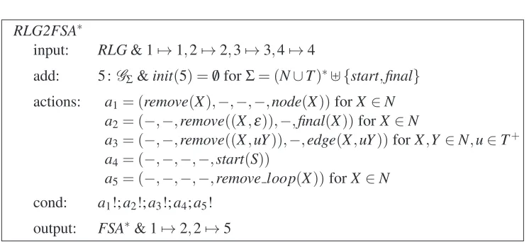
RLG2FSA∗
input: RLG& 17→1,27→2,37→3,47→4
add: 5 : GΣ&init(5) =/0 forΣ= (N∪T)∗⊎ {start,final}
actions: a1= (remove(X),−,−,−,node(X))forX∈N a2= (−,−,remove((X,ε)),−,final(X))forX∈N
a3= (−,−,remove((X,uY)),−,edge(X,uY))forX,Y∈N,u∈T+ a4= (−,−,−,−,start(S))
a5= (−,−,−,−,remove loop(X))forX∈N
cond: a1!;a2!;a3!;a4;a5!
output: FSA∗& 17→2,27→5
Figure 6: The model transformation unitRLG2FSA∗transforms right-linear Chomsky grammars (RLG) into finite state automata with word transitions (FSA∗)
− A model of the working type is a quintuple where the first four components of the working type correspond to the four types of a right-linear grammar; the last component is equal toGΣand serves to build up the finite state graph. It is initialized with the empty graph /0.
The alphabetΣmust equal(N∪T)∗⊎ {start,final}whereNare the nonterminal symbols
and T the terminal symbols of the input grammar, andstartand finalwill serve to label the start and final states of the finite state graph respectively.
− The input type declaration is composed of the constrained model type for right-linear grammars and the initializationinitial:[4]→set([5])withinitial(i) ={i}fori=1, . . . ,4. This means that the four components of the input type are the first four components of the working type. Hence, the four components of every input model are used as the first four components in the model the model transformation unit starts working with.
− The output type declaration consists of the constrained model typeFSA∗and the terminal-izationterminalwithterminal(1) =2 andterminal(2) =5. Hence, every output model of the unit is the pair consisting of the second and the last component of the model the unit ends working with, provided that the type of this pair equalsFSA∗.
− The set of actions ofRLG2FSA∗consists of five kinds of actions, each of which contains among other operations one of the graph transformation rules depicted in Figures4,5and
7.
1. The first actiona1= (remove(X),−,−,−,node(X))serves to generate a state in the graph for each nonterminal of the input grammar. More concretely, every application of this action generates a state with nameX while removing the nonterminalX from the set of nonterminals.
2. The second actiona2= (−,−,remove((X,ε)),−,final(X))inserts final pointers at all
start(S):
S S start
−→
final(X):
X X final
−→
remove−loop(X):
X
−→
Figure 7: Graph transformation rules for the actions of model transformation unitRLG2FSA∗
3. The third action a3= (−,−,remove((X,uY)),−,edge(X,u,Y))serves to generate transitions from those rules of the grammar that have a nonterminal in their right-hand side. Every application ofa3removes such a rule from the rule set in the third
component at the same time that a corresponding transition in the graph is generated.
4. Actiona4= (−,−,−,,start(S))inserts the start pointer at the stateSifSis the start symbol of the grammar.
5. Finally, the last action a5= (−,−,−,−,remove loop(X))forX ∈N serves to re-move all state names in order to obtain a finite state graph.
− The control conditiona1!;a2!;a3!;a4;a5! requires that at first all states be generated. This is achieved by applyinga1 as long as possible. The application ofa2as long as possible inserts for every rule with the empty word as right-hand side afinal-pointer while removing this rule. Thena3 requires to insert a transition for every remaining rule. Then the start state is inserted bya4and afterwards all state names are removed by applyinga5as long as possible.
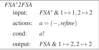
FSA∗2FSA
input: FSA∗& 17→1,27→2 actions: a= (−,refine)
cond: a!
output: FSA& 17→2,27→2
Figure 8: The model transformation unitFSA∗2FSAtransforms finite state automata with word transitions (FSA∗) into finite state automata (FSA)
If the input model ofRLG2FSA∗ is the right-linear grammar({S,A},{a,b,c},P,S) withP= {(S,aSa),(S,aA),(S,bbS),(A,cccA),(A,ε)}, the output model is ({a,b,c},G) where G is the
Finite state graphs with word transitions can be transformed into finite state graphs with sym-bol transitions by the model transformation unitFSA∗2FSAgiven inFigure 8.
The input type declaration consists of the constrained model typeFSA∗of finite state automata with word transitions and the initializationinitialthat maps the two components of every input model to the first two components of the working type. The working type of the unit is equal to
set(ID)×GΣ; the output type declaration consists of the model typeFSAfor finite state automata
and the terminalizationterminal, which is the identity in this case. The only actionaapplies the rulerefineofFigure 3to the graph component of the current model, while the control condition requires to apply the actionaas long as possible. If the input model ofFSA∗2FSAis equal to the state automaton({a,b,c},G)whereGis the finite state graph ofFigure 1, the output is equal to ({a,b,c},G′)whereG′is the finite state graph inFigure 2.
6
Sequential and Parallel Composition
Model transformation units can be used as building blocks for more complex model transforma-tion constructransforma-tions obtained by sequential and parallel compositransforma-tion. This leads to the notransforma-tion of model transformation expressions on the syntactic level. Semantically, the sequential composi-tion of model transformacomposi-tions is just the usual one of relacomposi-tions. And the parallel composicomposi-tion uses the fact that all models are considered as tuples of some product types so that the product of such types yields again models of some product type.
Definition 6(compositional expressions)
1. The setCX of compositional expressions is defined recursively:
(a) model transformation units are inCX,
(b) cx1, . . . ,cxk∈CX impliescx1;. . .;cxk∈CX (sequential composition),
(c) cx1, . . . ,cxk∈CX impliescx1k. . .kcxk∈CX (parallel composition).
2. The semantic relation of a compositional expression cx∈CX is defined according to its
syntactic structure:
(a) Ifcx=mtufor some model transformation unit, thenSEM(cx) =SEM(mtu). (b) If cx1;. . .;cxk for some model transformation units cxi with i=1, . . . ,k, then
SEM(cx1;. . . ;cxk) =SEM(cx1)◦. . .◦SEM(cxk)where
SEM(cxi)◦SEM(cxi+1)(m) =
[
m′∈SEM(cxi)
SEM(cxi+1)(m′)
for eachi∈ {1, . . . ,k−1}and eachmin the domain ofSEM(cxi).
(c) (m′1, . . . ,m′k)∈SEM(cx1k. . .kcxk)(m1, . . . ,mk)if and only ifm′i∈SEM(cxi)(mi)for
6.1 Examples
The sequential compositionRLG2FSA∗;FSA∗2FSAof the model transformation units inSection 5
transforms right-linear grammars into finite state automata so that the language generated by the input grammar is recognized by the automaton.
The formal language theory offers many examples of sequential compositions of model trans-formations like the transformation of right-linear grammars into finite state automata followed by their transformation into deterministic automata followed by the transformation of the latter into minimal automata.
A typical example of a parallel composition is given by the acception processes of two finite state automata that run simultaneously. If they try to accept the same input strings, this parallel composition simulates the product automaton that accepts the intersection of the two accepted regular languages.
To make the definition of compositional expressions more transparent, one may assign an input type and an output type to each compositional expression. Then the relational semantics of an expression turns out to be a relation between input and output types.
Definition 7(input and output types) The input type inand the output typeoutof a composi-tional expressioncx∈CX is recursively defined.
1. Ifcx=mtufor some model transformation unit with input typeIand output typeO, then
in(mtu) =I,out(mtu) =O,
2. If cx =cx1;. . .;cxk for some model transformation units cxi with i=1, . . . ,k, then
in(cx1;. . .;cxk) =in(cx1)andout(cx1;. . .;cxk) =out(cxk),
3. If cx =cx1 k. . .kcxk for some model transformation units cxi with i=1, . . . ,k, then
in(cx1 k. . .k cxk) =in(cx1)k . . .kin(cxk) and out(cx1 k . . .kcxk) =out(cx1) k. . .k out(cxk), where the parallel composition of model types is defined as follows
(a) (T kT′) = (T×T′)provided thatT andT′are free,
(b) T k(hT′with x′i) =h(T kT′)with x′iprovided thatT is free,
(c) (hT with xi)kT′=h(T kT′)with xiprovided thatT′is free, and
(d) (hT with xi)k(hT′ with x′i) =hT kT′with x∧x′i,
Due to these definitions, it is easy to see that compositional expressions describe transforma-tions from input models to output models.
Observation SEM(cx)(m)∈set(M(out(cx)))for allm∈M(in(cx)).
tr1
I1 O1 I2 tr2 O2
tr1;tr2
I1kI2
tr1 I1
tr2 I2
O1
O2
O1kO2
tr1ktr2
The sequential and parallel compositions on the level of model transformation expressions have the disadvantage that their results cannot be subject to further constraints. This is partic-ularly problematic with respect to the parallel composition because the composed units run in parallel, but without any interaction. This is quite all right provided that the components are meant to run independently of each other. But in many cases of parallel composition one intends that the components exchange information or process some data simultaneously. Such interre-lations and interactions could be achieved by adding further constraints and control conditions. This requires either to extend the notion of constraints and control conditions to the level of model transformation expressions or to flatten such expressions into model transformation units. The latter is done in the following.
6.2 Sequential Composition
Letmtui= (ITDi,OTDi,WTi,Ai,Ci) fori=1,2 be two model transformation units with input types Ii =hIi,1× · · · ×Ii,ki with xii and output types Oi =hOi,1× · · · ×Oi,ni with yii. By defi-nition of the semantics of the sequential composition mtu1;mtu2, the following holds: m′′= (m′′1, . . . ,m′′n2)∈SEM(mtu1;mtu2)(m) form= (m1, . . . ,mk1)∈M(I1) if and only if there is an
m′ with m′∈SEM(mtu1)(m) and m′′∈SEM(mtu2)(m′). This means in particular that m′ ∈
M(O1)∩M(I2)and thereforen1=k2. To avoid too much technical trouble, we assume in addi-tion thatWT=WT1=O1× · · · ×On1 =I1× · · · ×Ik2 =WT2. Then the sequential composition
ofmtu1andmtu2can be simulated by the model transformation unit
mtu(mtu1;mtu2) = (ITD1,OTD2,WT,A1∪A2,C(C1,C2,y1,x2,A1,A2))
where the control condition is chosen in such a way that a model transformation processm =∗⇒ A1∪A2
m′′is accepted if and only if it decomposes intom=⇒∗ A1
m′=∗⇒ A2
1. m=⇒∗ A1
m′is accepted byC1,
2. m′∈SEM(y1)∩SEM(x2),
3. m′=⇒∗ A2
m′′is accepted byC2.
Such a control condition may have the form of a transition system:
s0 s1 s2 s3
A∗1,C1 −,y1∧x1 A∗2,C2
requiring that at the beginning the actions of A1 are iterated regardingC1, that the result must
obeyy1andx2and that finally actions ofA2are iterated regardingC2.
It is not difficult to show that the following correctness result holds.
Observation SEM(mtu1;mtu2) =SEM(mtu(mtu1;mtu2)).
6.3 Parallel Composition
Letmtui = (ITDi,OTDi,WTi,Ai,Ci) fori=1,2 be two model transformation units each with input typeIi=hIi,1× · · · ×Ii,ki with xiiand initializationinitiali:[ki]−→set[li]as well as output typeOi=hOi,1× · · · ×Oi,ni with yiiand terminalizationterminal:[ni]−→[li]. Then the parallel composition ofmtu1andmtu2can be simulated by the model transformation unit
mtu(mtu1kmtu2) = (ITD,OTD,WT1×WT2,A,C)
where
− ITDconsists of the input typeI1kI2and the initializationinitiali:[k1+k2]−→set[l1+l2] with initial(i) =initial1(i) for i∈[k1]and initial(i) =l1+initial2(i−k1) for i=k1+ 1, . . . ,k1+k2,
− OTDconsists of the output typeO1kO2 and the terminalizationterminal:[n1+n2]−→
[l1+l2]withterminal(i) =terminal1(i)fori∈[n1]andterminal(i) =l1+terminal2(i−n1) fori=n1+1, . . . ,n1+n2,
− A=A1′×A2′withA1′=A1∪ {−}l1 andA2′=A2∪ {−}l2, and
− the control condition C is chosen in such a way that a model transformation process (m1,m2)=∗⇒
A (m1
′,m2′) is accepted if and only if it decomposes into m1 =∗⇒ A1′
m1′ and
m2
∗ =⇒
A2′
m2′ so that the former is accepted byC1 and the latter byC2 after removal of
The construction relies on the cartesian product of types and actions. Because the working type components 1 tol2become the componentsl1+1 tol1+l2, the initialization and terminalization
must be adapted accordingly. The actions of mtu1 and mtu2 are extended by the void action (−, . . . ,−)withl1andl2components respectively. This is necessary because the actions ofmtu1
andmtu2 may run in parallel, but the model transformation processes are of different lengths in
general so that they cannot run fully simultaneously.
It is again not difficult to show the following correctness result.
Observation SEM(mtu1kmtu2) =SEM(mtu(mtu1kmtu2)).
7
Related Work
In this section we briefly describe a selection of related work concerning model transformation. Since there exists quite an amount of publications we restrict ourselves to papers that are con-cerned with model transformations in the context of graph transformation. Moreover, we also mention some work that is concerned with the composition of model transformation definitions.
Model transformations based on graph transformation. One approach to define model transformations is by triple grammars [Sch94, KS06, SK08]. Each rule of a triple grammar can be easily transformed into a forward rule, a source rule, and a backward rule. The source rules are used to generate source models that – represented as graph triples – have the form (S,/0,/0) where S represents the source model. The forward rules are used to produce target models from source models. These target models – represented as graph triples – have the form (S,C,T)whereT is the target model. The backward rules are used to transform a target model (/0,/0,T)to a source model(S,C,T). In [EEE+07], it is shown that any source consistent model transformation based on triple grammars is backward information preserving. This means that the target model (generated by the forward rules of the grammar) can be transformed into the source model via the backward rules of the grammar. Roughly spoken, a model transformation MT is source consistent if there is a transformation that generates the source model from(/0,/0,/0) and that completely determines the matches in the source model of the forward rules applied in MT.
In [EE08], models are graphs equipped with a semantics given as a set of simulation rules, and a model transformation is composed of generating first an integrated model by graph trans-formation rules and restricting it then to the target model. It is shown under which conditions semantical correctness and completeness of model transformations are achieved. In [K ¨us06], an approach to model transformation is presented that uses transformation units based on typed attributed graph transformation. It provides criteria for syntactic correctness as well as for termi-nation and confluence.
Examples of model transformation tools based on graph transformation are VIATRA2 [VB07], GReAT [BNvBK06] and ATOM3[dLVA04]. VIATRA2 integrates graph transformation and
in-terfaces where the former can receive graph objects from previous rules and the latter can send graph objects to another rule. ATOM3focuses on modeling complex systems composed of var-ious formalisms and allows to transform them into a single common formalism based on graph transformation. In [dLT04], ATOM3is combined with AGG for validation purposes.
In general, the mentioned publications on model transformation with graph transformation are very close to our approach – they are however restricted to transform mainly graphs, not tuples of graphs, sets or sequences as proposed in this paper.
Composition of model transformations. In the literature one can find two main types of composition techniques for model transformation definitions: external and internal composition. The first one chains model transformations sequentially whereas the second composes the rules of a set of model transformation definitions into one transformation definition. In this sense the compositions presented in Subsections6.2and6.3can be considered as internal compositions.
In [Wag08], the composition of model transformation definitions via superimposition is de-scribed, which is a feature of the ATLAS Transformation Language [JK05]. Superimposition of modules is an internal composition technique where models can be superimposed on top of each other yielding a module that contains the union of all transformation rules. In [YCWD09], the au-thors consider composition of model transformation definitions that transform high-level models into low-level models by defining a correspondence model that specifies the relations between the high-level meta models. The low-level correspondence model is automatically generated so that the low-level models can be composed homogeneously. In this way, new concerns can be added to existing model transformation definitions. In [CM08], two approaches for reusing model transformation definitions are proposed. The first one is called factorization and it al-lows to extract common parts of model transformation definitions obtaining in this way a base transformation definition which can be reused. The second concerns composition of transfor-mation definitions which have compatible source metamodels but different target metamodels. Metamodels are related via small new metamodels and the transformations are integrated via an integration transformation definition that locates and connects the join points (without know-ing the rules but some kind of trace information) by usknow-ing so-called refinement rules. One ap-proach towards composition of model transformations based on graph transformation is studied in [BHE09] where models are typed graphs that are mapped to semantic domains. The authors define spatial compositionality of semantic mappings which roughly spoken means that the se-mantics of a model is equal to the sese-mantics that is obtained by embedding the sese-mantics of a piece of the model into some context. It is assumed that the semantic mappings are graph transformation systems with a functional behavior and it is shown under which conditions they behave compositionally. In [KKS07], a first approach towards structured model transformation is proposed that allows package import, package merge and generalization according to a stan-dardized packaging concept of the UML. In particular, the authors extend triple graph grammars by the mentioned concepts.
8
Conclusion
sets, numbers, etc. Models of this kind cover graphical models like UML diagrams as well as set-theoretic models like grammars and automata. They are transformed componentwise by rule applications in the cases of graphs and by applications of data type operations in the other cases. Besides a set of such actions, a model transformation unit provides descriptions of input, output, and working models as well as a control condition to regulate the use of actions. Semantically, a transformation of input models into output models is specified. Moreover, we have studied sequential and parallel compositions of model transformation units as means to build up complex transformations from simple ones.
Although the considerations in this paper seem to be promising, more work is needed to un-derpin the significance of this novel approach, including the following points.
1. As pointed out in Section 4, the introduced kind of model transformation is nondeter-ministic. Therefore, sufficient conditions are often of interest that guarantee termination, completeness and functionality where the first property means that there is no infinite run, the second one requires at least one output for each input, and the latter one requires at most one output for each input.
2. Concerning our running example, it is known from the literature that a right-linear gram-mar generates the same language as is recognized by the finite state automaton resulting from the transformation. One intention of our approach is to support such correctness proofs. Therefore, notions of correctness and an appropriate proof theory must be studied in the future.
3. An interesting question in this respect is whether and how these correctness notions are compatible with the sequential and parallel compositions so that the correctness of the components yields the correctness of the composed model transformation.
4. Further explicit and detailed examples are needed to illustrate all introduced concepts more convincingly, in particular examples for parallel and sequential composition with interac-tion between components.
Acknowledgments We are grateful to the unknown referees for various helpful comments. The first author wants to thank Hartmut Ehrig for the long lasting cooperation and friendship. Hans-J¨org (being a Math student at the time) met Hartmut in 1970 when a very close relation-ship started. Hartmut supervised Hans-J¨org’s diploma thesis in 1974 and his PhD thesis in 1978. Moreover, he guided Hans-J¨org to habilitation in 1981. Hartmut introduced Hans-J¨org to cate-gory theory. They both learned automata theory together. Hartmut convinced Hans-J¨org of the significance of graph transformation. They both together got involved in algebraic specification. Although this happened in the 1970s, it sticks: Elements of all four areas can be found in the present paper. Hans-J¨org happily acknowledges that he is one of Hartmut’s grateful students.
Bibliography
[BNvBK06] Daniel Balasubramanian, Anantha Narayanan, Christopher P. van Buskirk, and Ga-bor Karsai. The graph rewriting and transformation language: GReAT.ECEASST, 1, 2006.
[CHK04] Bj¨orn Cordes, Karsten H ¨olscher, and Hans-J¨org Kreowski. UML interaction dia-grams: Correct translation of sequence diagrams into collaboration diagrams. In John l. Pfaltz, Manfred Nagl, and Boris B ¨ohlen, editors,Applications of Graph Transfor-mations with Industrial Relevance (AGTIVE 2003), volume 3062 ofLecture Notes in Computer Science, pages 275–291, 2004.
[CM08] Jes´us S´anchez Cuadrado and Jes´us Garc´ıa Molina. Approaches for model transfor-mation reuse: Factorization and composition. In Vallecillo et al. [VGP08], pages 168–182.
[dLT04] Juan de Lara and Gabriele Taentzer. Automated model transformation and its val-idation using AToM3 and AGG. In Alan F. Blackwell, Kim Marriott, and Atsushi Shimojima, editors, Diagrammatic Representation and Inference, volume 2980 of
Lecture Notes in Computer Science, pages 182–198. Springer, 2004.
[dLVA04] Juan de Lara, Hans Vangheluwe, and Manuel Alfonseca. Meta-modelling and graph grammars for multi-paradigm modelling in AToM3. Software and System Modeling, 3(3):194–209, 2004.
[EE08] Hartmut Ehrig and Claudia Ermel. Semantical correctness and completeness of model transformations using graph and rule transformation. In Ehrig et al. [EHRT08], pages 194–210.
[EEE+07] Hartmut Ehrig, Karsten Ehrig, Claudia Ermel, Frank Hermann, and Gabriele Taentzer. Information preserving bidirectional model transformations. In Matthew B. Dwyer and Ant´onia Lopes, editors,FASE, volume 4422 ofLecture Notes in Computer Science, pages 72–86. Springer, 2007.
[EHRT08] Hartmut Ehrig, Reiko Heckel, Grzegorz Rozenberg, and Gabriele Taentzer, editors.
Graph Transformations, 4th International Conference, ICGT 2008, Leicester, United Kingdom, September 7-13, 2008. Proceedings, volume 5214 of Lecture Notes in Computer Science. Springer, 2008.
[Fra03] David S. Frankel.Model Driven Architecture. Applying MDA to Enterprise Comput-ing. Wiley, Indianapolis, Indiana, 2003.
[HKK09] Karsten H ¨olscher, Hans-J¨org Kreowski, and Sabine Kuske. Autonomous units to model interacting sequential and parallel processes. Fundamenta Informaticae, 92(3):233–257, 2009.
[KHK06] Hans-J¨org Kreowski, Karsten H ¨olscher, and Peter Knirsch. Semantics of visual mod-els in a rule-based setting. In R. Heckel, editor,Proceedings of the School of SegraVis Research Training Network on Foundations of Visual Modelling Techniques (FoVMT 2004), volume 148 ofElectronic Notes in Theoretical Computer Science, pages 75– 88. Elsevier Science, 2006.
[KK99] Hans-J¨org Kreowski and Sabine Kuske. Graph transformation units with interleaving semantics. Formal Aspects of Computing, 11(6):690–723, 1999.
[KKR08] Hans-J¨org Kreowski, Sabine Kuske, and Grzegorz Rozenberg. Graph transformation units – an overview. In P. Degano, R. De Nicola, and J. Meseguer, editors, Con-currency, Graphs and Models, volume 5065 ofLecture Notes in Computer Science, pages 57–75. Springer, 2008.
[KKS97] Hans-J¨org Kreowski, Sabine Kuske, and Andy Sch¨urr. Nested graph transformation units. International Journal on Software Engineering and Knowledge Engineering, 7(4):479–502, 1997.
[KKS07] Felix Klar, Alexander K ¨onigs, and Andy Sch¨urr. Model transformation in the large. In Ivica Crnkovic and Antonia Bertolino, editors,ESEC/SIGSOFT FSE, pages 285– 294. ACM, 2007.
[KS06] Alexander K ¨onigs and Andy Sch¨urr. Tool integration with triple graph grammars - a survey. Electr. Notes Theor. Comput. Sci., 148(1):113–150, 2006.
[K ¨us06] Jochen Malte K ¨uster. Definition and validation of model transformations. Software and System Modeling, 5(3):233–259, 2006.
[OMG08] OMG. Meta object facility (MOF) 2.0 query/view/transformation (QVT). http://www.omg.org/spec/QVT/, 2008.
[Sch94] Andy Sch¨urr. Specification of graph translators with triple graph grammars. In Ernst W. Mayr, Gunther Schmidt, and Gottfried Tinhofer, editors,Graph-Theoretic Concepts in Computer Science, volume 903 of Lecture Notes in Computer Science, pages 151–163. Springer, 1994.
[SK08] Andy Sch¨urr and Felix Klar. 15 years of triple graph grammars. In Ehrig et al. [EHRT08], pages 411–425.
[VB07] D´aniel Varr´o and Andr´as Balogh. The model transformation language of the VIA-TRA2 framework. Science of Computer Programming, 68(3):187–207, 2007.
[VGP08] Antonio Vallecillo, Jeff Gray, and Alfonso Pierantonio, editors. Theory and Prac-tice of Model Transformations, First International Conference, ICMT 2008, Z¨urich, Switzerland, July 1-2, 2008, Proceedings, volume 5063 ofLecture Notes in Computer Science. Springer, 2008.