Bulk Material Terminal Simulation Modeling

(1)

Bulk Material Terminal Simulation Modeling

Mohammad Mahdi Badiozamani and Hooman Askari-Nasab

Mining Optimization Laboratory (MOL)

University of Alberta, Edmonton, Canada

Abstract

Bulk terminals are designed to facilitate the material flow from mines to plants in a network of mining facilities and receiver plants. Therefore, such terminals are considered to be one of the most important nodes in mining logistic networks. Optimal design of such terminals has a dominant effect on the success rate of mining material supply chain. In the literature, a number of mathematical models are developed to decide on the optimal design and schedule of such terminals. However, due to the presence of high uncertainty in real terminal operations, such deterministic models fail to deliver reliable solutions. Simulation is a useful technique to capture the uncertainty existing in the arriving material contents and terminal operations such as unloading, sampling, sorting, stacking, reclaiming and loading operations. In this paper, a simulation model is developed for a typical iron ore bulk terminal. The terminal is consisted of three main parts as; train unloading section, stockyard area and vessel loading section. An Arena model is developed to capture the performance measures of these three terminal sections, specifically the mean and maximum values for the inventory level of cells and total waiting time for any single train to be unloaded and vessel to be loaded. The number of replications is adjusted in a way to increase the accuracy of the estimations for the desired performance indicators. The proposed simulation model is capable of testing different cell allocations in the stock yard area and also more complex scenarios about stacking/reclaiming functions. The model is verified and the results are presented and discussed. As the further step, the proposed model should be validated, based on the real parameters and input data from a bulk material terminal.

1. Introduction

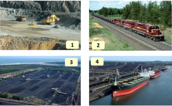
Designing a proper logistic network that facilitates the shipment and storage of the mined material is considered to be an important task in mining supply chain management. This network consists of two main elements; nodes and arcs. The nodes represent all of the facilities in the network such as mining and processing plants (the supply side), the production plants as a final destination of the material (the demand side) and finally, some transshipment points such as bulk material terminals that facilitate the transfer of the mined/processed material to the destinations. In fact, the terminals balance the demand and supply flows through the network. The arcs represent the routes that interconnect different nodes in the network together. Some sample views from the network are illustrated in Fig. 1. One critical decision making problem for the network design is to determine the number, location, size and design of terminals. Designing such terminals is considered to be important from two points of view; balancing the material flow in the network and also cost reduction aspects. The design and capacity of terminals mostly depends on the input rate (from suppliers) and the output rate of commodity (from demand points). In reality, due to the uncertainty existing in schedules of transportation facilities such as trains and vessels, both input rate to the terminal and output rate from it may follow stochastic patterns.

(2)

In the literature, one can find this issue under the category of logistics management and more specifically, the inventory management. Different approaches are developed to evaluate the performance of bulk terminals. In many of related works, the focus is on the coal terminal which represents other bulk solid material terminals as well. In some of them, the focus is on development of an exact mathematical model for terminal operations, while others concern more about finding a reliable solution through heuristic approaches to solve such large scale mathematical models.

Fig. 1. Iron ore supply network.

Abdekhodaee et al. (2004) investigate a typical coal terminal problem and divide the whole terminal system into two sub-systems; railing sub-system and stockyard sub-system. For each of these sub-systems, an integer programming (IP) formulation is developed that works properly for small scale problems. The railing IP model minimizes the summation of penalties that are applied to any violation from trains’ schedule. The stockyard IP model minimizes the summation of conflicts that happen during stacking and reclaiming operations in the stockyard (section 3). As a result, the proposed IP model for stockyard system allows physical infeasibilities to be scheduled, but minimizes them. In order to solve the model for large scale problems in a reasonable time, a greedy heuristic algorithm is developed to find the solution. Simulation results are used in proposed heuristic.

In presence of uncertainty, one powerful technique that can be applied to investigate performance of the system is discrete event simulation. The first step in building a simulation model is to determine different components of the system, which in this case is a typical bulk solid material terminal. All bulk terminal activities can be categorized in four groups as; (1) receiving, (2) storing, (3) blending and (4) shipping activities.

Weiss et al. (1999) discuss the implementation of simulation techniques for solid bulk material terminals and review different simulation components that are required to model all four different activities of a terminal in more details as the followings:

1) Stockpiling area: occupies most of the terminal area and is partitioned in order to avoid any probable dilution and contamination due to mixing different material.

2) Rail facility: provides required area and facility for arriving trains which have brought the bulk load to the terminal.

(3)

3) Ship loading facility: consisted of berths and docks to accommodate both relatively small ships and ocean-going vessels.

4) Stacking – reclaiming: installed between stockpiles and are used to stack the trains load

into the stockpiles or reclaim the material from stockpiles and send it to the quays.

5) Other process facilities: crushing and sizing small plants, drying plants, power plants and other required logistical facilities in the terminal.

6) Conveyor system: complex belt system which connects other facilities of the terminal. In this paper, some of initial steps to simulate a solid bulk material terminal are presented and an Arena simulation model (Arena, 2009) is developed for the purpose. The paper has the following sections: Problem definition is presented in section 2. A sample mathematical model is presented in section 3. The proposed simulation model, in details with its components is discussed in section 4. Model verification is presented in section 5 and the results are discussed in section 6. Finally, future steps in validating the terminal model and testing more scenarios are discussed in section 7.

2. Problem definition

In an overall point of view, an iron ore terminal receives ore with different qualities from one or a number of mines. Then, the ore is stocked in proper stockpiles and sent to a number of quays to be loaded into the vessels. More specifically, following operations and activities take place in the iron ore terminal:

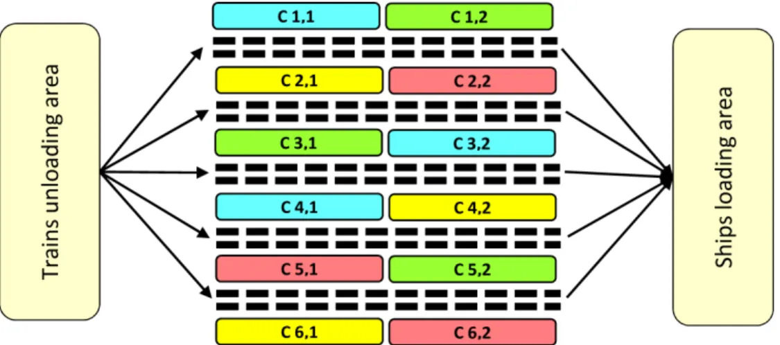
The ore is shipped from different mines by trains. It is assumed that each train has a capacity of 3000 tonnes and trains arrive into the terminal in three shifts (Table 1). The trains’ load is then unloaded, using a number of unloaders, and sent for sampling to determine the specifications of the load and its type. Sampling time follows a Normal distribution with mean of 1 hour and standard deviation of 30 minutes. According to the sampling results, the proper cell for each load in the terminal is determined. It is assumed that each arriving load has an equal chance to be either of types A, B, C or D (each with chance of 25%). The load is sent to the proper stockyard cell via a network of conveyors. The stockyard is partitioned into 12 separated cells to avoid any dilution and mixture of different quality ore types. Four different ore types can be stocked in these cells (three cells for each kind of iron ore). Stackers are used to dump the material into proper cell. A schematic view of the terminal, including the train unloading section, stockyard cells and ships loading section, is illustrated in Fig. 2.

(4)

On the other hand, the loading process is triggered by receiving a load order from customer. Orders are received by the terminal 24 hours a day and the time between order arrivals is eight hours. Same to the arriving loads, the orders have an equal chance to be for ore types A, B, C and D (each with chance of 25%).

Table 1. Trains’ first arrival times. First arrival time

Shift 1: Triangular (12:00 AM , 04:00 AM , 08:00 AM) Shift 2: Triangular (08:00 AM , 12:00 PM , 04:00 PM) Shift 3: Triangular (04:00 PM , 08:00 PM , 12:00 AM)

Based on the records and due to real unstable conditions of the ocean, ships arrive into the terminal, not exactly when the orders are received. Since the loading to the ships can only be initiated when the order and corresponding ship are present in the terminal, the order is held until the corresponding ship arrives. The inter arrival time for ships follows a triangular distribution as (7.5 , 8.0 , 8.5) hours. In the simulation model, it is assumed that the first order and the first ship are arrived randomly with a triangular distribution between 3:00 AM to 7:00 AM, with the most chance for 5:00 AM. There are three quays in the terminal. 30% of ships are assigned to quay 1, 40% to quay 2 and 30% to quay 3. Four ships can be loaded at the same time at each quay. When the ship with predetermined order berths, the reclaimers load the dumped ore from proper cell into the conveyor belt. The belts are designed in a way to load the coal into the ships that are berthed in quay. As a result, the ore is loaded into the ship based on the specified amount and quality of the order. The tonnage for each order is assumed to be 6000 tonnes.

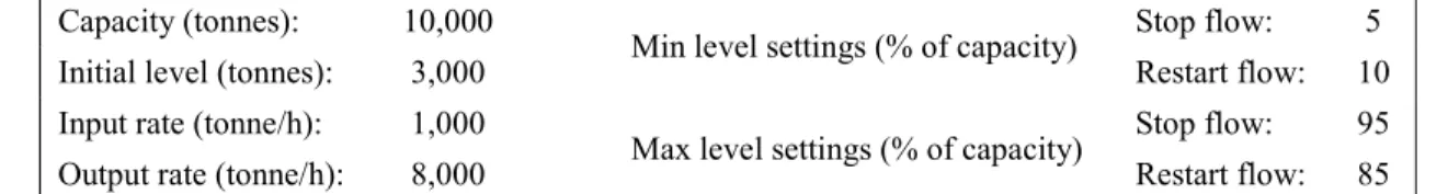
When loading of the ships finishes, the ship decouples from the quay and it takes a time with Normal distribution with a mean of one hour and standard deviation of 15 minutes. To prevent any unexpected shut downs of the terminal flow, it is decided to stop the flow of material to the cells when the level of each cell reaches to 5% of its capacity and restart it when it reaches to 10% of capacity. On the other hand, to avoid any overflow of the cells, it is assumed that the flow to the cells becomes zero when the level of each cell reaches to 95% of its capacity and restarts when it reaches to 85% of capacity. The complete data about the capacity of terminal cells, the input rate, output rate and the initial level of ore in each cell is presented in Table 2.

Table 2. Specification of cells. Capacity (tonnes): 10,000

Min level settings (% of capacity) Stop flow: 5

Initial level (tonnes): 3,000 Restart flow: 10

Input rate (tonne/h): 1,000

Max level settings (% of capacity) Stop flow: 95

Output rate (tonne/h): 8,000 Restart flow: 85

The aim is to develop a simulation model for the terminal which makes testing different scenarios possible. Specifically, the key performance indicators (KPIs) considered to evaluate the performance of the terminal are as follows:

• Utilization of quays,

• Total waiting time for ships and trains in the terminal,

• Average number of ships and trains being served in the terminal, • Minimum, maximum and average of ore inventory in each cell.

Since the bulk material in terminal is carried by conveyor belts smoothly and in a very constant rate, the system can be assumed to be continuous and the cells can be modeled as tanks.

(5)

3. Mathematical formulation

Some mathematical programming models are developed to find the exact and optimal design for the terminal. As an example, Abdekhodaee et al. (2004) consider the supply network as a combination of two sub systems, the railway system and the coal terminal system. Two integer programming formulations are developed to optimize performance of each sub system. Although the model is developed for a coal terminal, the same concept works for almost every solid bulk material. The integer programming objective is to minimize the total number of conflicts that may occur during stacking and reclaiming activities. The basic inputs in this model are the different types of products, opening and closing times for stockpiles, stackers and reclaimers. Pairs of (r,m) are used to identify the row number and dimension (in meters) of each stockpile. Three types of opening and closing time intervals are considered as following:

1 1

[ ,to tc_i _i): an interval beginning at the time a stockpile becomes ready to receive coal for storage, and ending at the time that this stockpile is available to receive a new product.

2 2

[to tc_i, _i): an interval over which a stacking operation occurs.

3 3

[to tci, i): an interval over which a reclaiming operation occurs.

For instance, for the list of products P = {1, 2, 3, 2}, There will be a corresponding list of stockpile opening-closing times _{[ ,}1 1₎

i i

to tc given by 1 _{{(1,15),(3,18),(9,21),(12,21)}}

OC

T = . It is assumed that

pre-designated stockpile locations are assigned to different products in the terminal. So, a particular product may be permitted for instance in stockpiles at locations ( , ) {(1,11),(1,7),(3,7),(2,10)}r m ∈ . “S” is defined as the union of these sets of permissible stockpile locations.

i P

S : the set of possible stockpiles for a productPi.

,

r m

K : the set of machines that can access stockpile (r,m). j

K : the set of machines allocated to row (bund) j.

,

k m

d : the distance of a stockpile from the end of its row, in the direction of machine k (there are generally two stacker/reclaimer machines in each row).

Three zero-one decision variables are defined as:

, , ,

r m i t

Y : Is one, if i-th item in product list is allocated to position (r,m) in the stockyard at time t

and zero, otherwise.

, , ,

k m i t

X : Is one, if i-th opening-closing for stacking machines is allocated and zero, otherwise.

, ,

k i t

Z : Is one, if i-th opening-closing for reclaiming machines is allocated and zero, otherwise. Finally, Decision variable i

t

C is defined as the number of conflicts occurs in different terminal sections in each period. The proposed formulation allows scheduling of physical infeasibilities, but tries to minimize them.

1 2 3

( t t t )

Min

∑

C +C +C (1)

1

, , , i 1 ( , ) Pi r m i to

r m

Y = ∀i and r m S∈

∑∑

(2)

1 1 1

, , , , , , _i , , [ , )

r m i t r m i to i i

(6)

1 2 2

, , , _{, , ,} _i , [ , ) ,

k m i t _{r m i to} i i r m

k m

X =Y ∀ ∈i t to tc and k K∈

∑∑

(4)

1 3 3

, , , , , , i , [ , ) ,

k m i t _{r m i to} i i r m

k m

Z =Y ∀ ∈i t to tc and k K∈

∑∑

(5)

1

, , , 1 , ,

r m i t t i

Y ≤ +C ∀r m t

∑

(6)

2 , , , , , ,

( k m i t k m i t) 1 t , m i

X +Z ≤ +C ∀k t

∑∑

(7)

3 , , , , , , ,

( ) 1,...,

j

k m i t k m i t t j

k K m i

X Z MS BL C t and j r

∈

+ + ≤ + ∀ =

∑ ∑∑

(8)

Eq. (1) defines the objective function of the model that is to minimize the total number of conflicts in the system. Eqs. (2) and (3) allocate a product (parcel) to a location (r,m) and retain the allocation throughout the opening and closing of that parcel. Eq. (4) allocates a stacking operation to a machine, while Eq. (5) allocates a reclaiming operation to a machine. The next three constraints deal with the number of possible conflicts. Eq. (6) measures the possible number of conflicts in assigning different overlapping parcels to a single stockpile. Eq. (7) calculates the number of conflicts in assigning overlapping reclaiming and stacking tasks to a single machine. Finally, Eq. (8) determines the amount of conflict in machines-on-the-same-bund movement (where MS is the minimum separation between machines and BL is the bund length). By introducing different weight coefficients, it is possible to change the relative importance for different types of conflicts.

Since the proposed integer programming formulation is not practical for large scale problems, the model is used for just small size problems. To solve the large scale problems, a heuristic algorithm is developed which uses simulation results in its iterations.

4. Simulation model

Arena (2009) is a powerful simulation package and is used in this paper for building the simulation model to study the performance of the terminal in presence of uncertainty. Stockyard cells and conveyor belts are modeled with the flow process modules of Arena, which is a powerful tool for simulating the continuous behavior of input and output rates. The model is consisted of three main parts as; (1) train unloading section, (2) ship loading section and (3) stockyard area.

Dumping of arriving loads to the stockyard cells is modeled in the train unloading section. The entity in this section is the train load, which has four attributes; load size, iron ore grade, phosphor grade and sulfur grade. During each 8 hour shift, one train arrives in the railway station, but the first arrival time is not always the same and follows a probability distribution function. A sampling process is done for each arriving load to verify the grades. Then according to the grade distributions, the load is directed to the proper stockyard cells through conveyor belts. There are three cells corresponding to each grade quality. These cells are selected in a random order for the loads with that specific grade range. The train load entity is disposed when the load is conveyed completely to the cells. The Arena model for train unloading section is illustrated in Fig. 3.

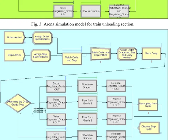
On the other hand, the ship loading section covers different processes that are triggered when a load order arrives. It is assumed that the orders are received almost always earlier than corresponding ship arrival time. That is because of the nature of oceanic transportation. As a result, the terminal freezes each order until its corresponding ship arrives and then, lets the order/ship wait to be loaded. Same to the train load entities, corresponding attributes are defined for each ship load

(7)

entity as order size, order quality (grade) and the quay number which the ship is going to be loaded at. According to the quay assignment, ships line up in corresponding queue to be loaded. Each quay can load four ships at the time. When loading finishes, the ships are decoupled from the quay and leave the loading dock. Ship load entity is disposed when the ship leaves the terminal. The Arena model for ship loading section is illustrated in Fig. 4.

Fig. 3. Arena simulation model for train unloading section.

(8)

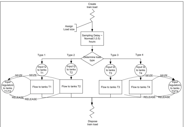
Flow to tanks T1

Assign Load size

Create train load

Sampling Delay ~ Normal(1,0.5) hours Determine load type Type 1 Input Q to tanks T1

Flow to tanks T4

Input regulators to tanks T3/T4 SEIZE RELEASE Input Q to tanks T4 Type 4 Dispose train load

Flow to tanks T3 Input Q to tanks T3

Flow to tanks T2 Input Q to tanks T2

Type 2 Type 3

SEIZE RELEASE Input regulators to tanks T1/T2 SEIZE RELEASE SEIZE RELEASE

Fig. 5. Logic flow chart for train unloading section.

Flow to tanks T1 Assign Order number Input regulators to T1/T2 SEIZE RELEASE Create order

Match order and ship based on their numbers &

Create ship load

What is order type Input Q

to tanks 1

Flow to tanks T4 regulators Input to T3/T4 SEIZE RELEASE Input Q to tanks 4 Type B Dispose ship load Assign ship number Create ship Q for match and batch Assign Order type, order size and quay number Decoupling Delay ~ Normal(1,0.25) hours quay SEIZE RELEASE Quay Q Type 1

Flow to tanks T2 Input Q to tanks

2

Flow to tanks T3 Input Q to tanks 3 SEIZE RELEASE SEIZE RELEASE

(9)

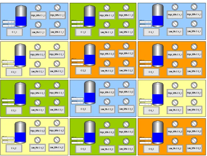
Logic flow charts for train-unloading and ship-loading sections are presented in Figs. 5 and 6, respectively. For more details on the steps of creating the model, see paper 402. Add a sentence referring the reader to paper 402 for detailed modeling. The stockyard section is consisted of 12 separated cells. Each three of these cells are assigned to a specific iron ore quality. The train load is conveyed into the proper cell and stacked in it by the means of stackers. On the other hand, when an order/ship arrives, using reclaimers, the ore is reclaimed from the cell, convoyed to the proper quay and loaded into the ship. It is assumed that each cell had its own stacker and reclaimer. To simulate stacking and reclaiming processes in the cells, each cell is considered as a tank which has an input regulator (conveyor and stacker) and an output regulator (reclaimer and conveyor). All of the tanks have the same capacity and almost one third of their capacity is full when the simulation initiates. There are two rules for stacking to and reclaiming from each cell. In order to avoid any dilution or mix between neighbor cells, the input flow to the cell should be stopped when 95% of cells capacity is full and can be restarted when its inventory reaches to 85% of the capacity. On the other hand, the output flow from the cell should be stopped when 5% of cells capacity is remaining and can be restarted again when its inventory reaches to 10% of capacity. The Arena model for stockyard section is illustrated in Fig. 7. Different colors represent different grade qualities that are contained in the cells.

Fig. 7. Arena simulation model for stockyard section. The following Arena modules are used in building the terminal model:

• Create: to create train load, order and ship entities.

• Assign: to define required variables and attributes for the entities through the model.

• Process: to introduce processes take place in the model, including sampling train loads and

(10)

• Decide: to distinguish between different load and order qualities in train unloading and ship loading sections.

• Seize regulator: to seize cells’ input regulators in train unloading section and output

regulators in ship loading section when the flow starts.

• Flow: to make the flow to and from the cells in train unloading and ship loading sections.

• Release regulator: to release cells’ input regulators in train unloading section and output

regulators in ship loading section when the flow stops.

• Match: to hold ship and order entities until they match together and let them move in the

model.

• Batch: to batch ship and order quantities when they are match together and make a new

entity (ship load).

• Tank: to represent cells capacity and filling/emptying behavior. • Sensor: to capture stop/restart levels in the cells (tanks). • Dispose: to dispose the train load and ship load entities.

5. Model verification

Prior to run the model, it is first required to make sure that the mass of material that is flowed in the terminal is balanced. Eq. (9) defines the material mass balance in the terminal.

i i i i i

in I out W F

M +L =M +M +L (9)

Where; i in

M is the mass of ore type i that enters into the terminal (tonne), i

out

M is the mass of ore type i that leaves the terminal (tonne), i

W

M is the mass of ore type i that has entered into the terminal, but is waiting to be unloaded (tonne),

i I

L is the initial level of tanks for ore type i when the simulation starts (tonne), i

F

L is the final level of tanks for ore type i when the simulation ends (tonne).

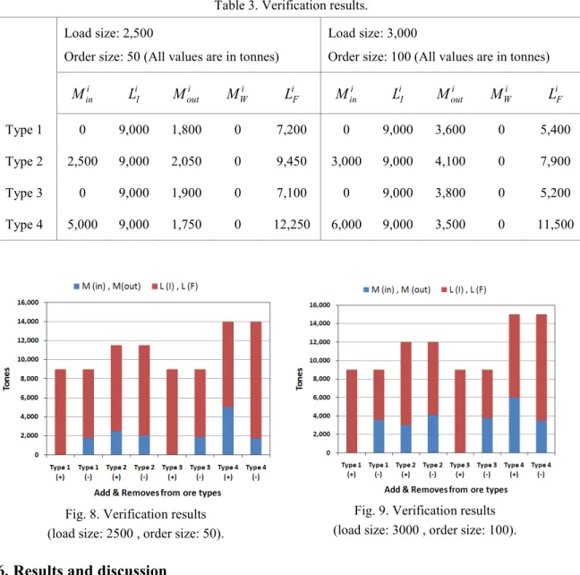
The model is run with different values for train load sizes and ship order sizes. Eq. (9) is the checked for each pair of train and ship load sizes. The results for two cases are reported in Table 3. The results show that the material in the model is completely balance, meaning that the total amount of input plus the initial tank levels adds up with the total amount of output, plus the final tank levels and waiting loads in the terminal. These values confirm that the model is performing right in terms of material mass balance. The results are also illustrated in Figs. 8 and 9.

(11)

Table 3. Verification results. Load size: 2,500

Order size: 50 (All values are in tonnes)

Load size: 3,000

Order size: 100 (All values are in tonnes) i

in

M i

I

L i

out

M i

W

M i

F

L i

in

M i

I

L i

out

M i

W

M i

F

L

Type 1 0 9,000 1,800 0 7,200 0 9,000 3,600 0 5,400

Type 2 2,500 9,000 2,050 0 9,450 3,000 9,000 4,100 0 7,900

Type 3 0 9,000 1,900 0 7,100 0 9,000 3,800 0 5,200

Type 4 5,000 9,000 1,750 0 12,250 6,000 9,000 3,500 0 11,500

Fig. 8. Verification results (load size: 2500 , order size: 50).

Fig. 9. Verification results (load size: 3000 , order size: 100).

6. Results and discussion

Number of replications:

The terminal model is run for 13 days and simulation base time unit is in hours. In order to decide on the proper number of replications, two important KPIs of the terminal are taken into account; (1) the total time that it takes to unload a train completely and (2) the total time that it takes to load a ship. Since these two are the most important measures in assessing the terminal performance, reduction of the uncertainty in estimation of these KPIs is a goal. In other words, the half-widths for these two KPIs should be considered in determining the number of replications. Eq. (10) is used to find the proper number of replications:

2 0 0 ( )h

n n h

= × ₍₁₀₎

Where _nand n 0 are the proper and test numbers of replications, respectively and hand h 0 are the

corresponding half widths. In order to reach into the half widths of 3 minutes for the trains total unloading time and 30 minutes for the ships loading time, Eq. (10) results in following numbers of replications:

(12)

2 2 0

0 ( ) 10 (0.08_0.05) 25.6 26

train

train train train

train

h

n n n

h

= × = × = _

2 2

0

0 ( ) 10 (0.96_0.50) 36.86 37

ship

ship ship ship

ship

h

n n n

h

= × = × = _

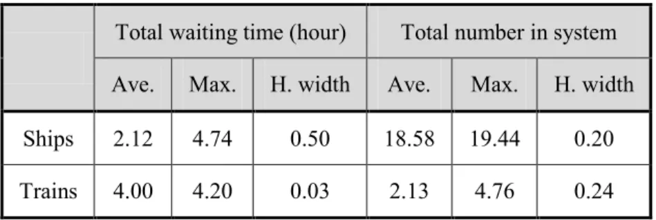
After running the model for 37 replications, it turns out that few more replications are required in order to reach to 30 minutes half width for ship loading time. Therefore, 39 replications are considered for this model. The entity-related results from 39 replications are presented in Table 4. According to these results, on average, total number of trains in the terminal are much less than the total number of ships. However, the average total time that a train spends in the terminal to be fully unloaded is four hours on average, which is almost twice the same value for the ships. It can be inferred from these numbers that any improvement in unloading facilities may result in smaller waiting time of the trains. In addition, in some cases there exist some considerations which do not let the filling and emptying of the cells take place simultaneously. In such cases, any upgrade in either sides of cells input or output flows may improve another as well. In general, higher input rate to the cells will result in smaller trains waiting time and number of trains hold in the terminal. The same statement is true for the ship loading section as well.

The utilization of quays is reported in Table 5. All three quays have the same capacity of four loading docks. According to these values, the average utilization of second quay has been more than two others. That is because of the quays assignments pattern to the ships. Since the first and third quays are planned to have some maintenance activities, 60 percent of ships are assigned equally to the first and third quays (30 percent to each one), while 40 percent of ships are sent to the second quay. The total number of times that each of three quays are seized are almost equal.

Table 4. Simulation results (based on entities).

Total waiting time (hour) Total number in system Ave. Max. H. width Ave. Max. H. width Ships 2.12 4.74 0.50 18.58 19.44 0.20 Trains 4.00 4.20 0.03 2.13 4.76 0.24

Table 5. Simulation results (resources utilizations). Utilization (%) Total number seized Min. Ave. Ave. Max. Quay 1 53.12 79.23 4.36 7 Quay 2 56.88 84.68 4.31 6 Quay 3 16.70 74.66 4.51 7

(13)

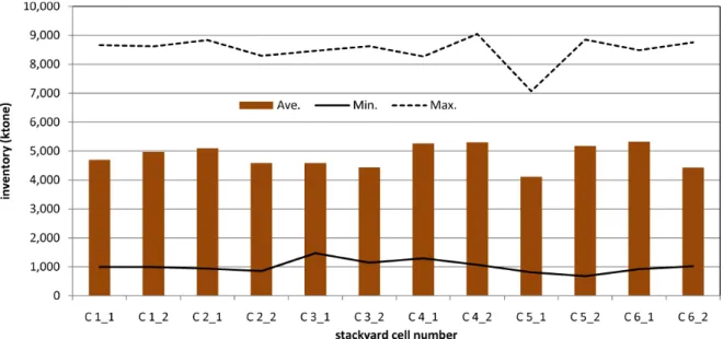
Table 6. Simulation results (cells' inventories / tank levels). Cell (tank)

name

inventory (ktonne) _{Cell (tank)} name

inventory (ktonne)

Min. Ave. Max. Min. Ave. Max.

C 1_1 997.13 4696.14 8667.20 C 4_1 1295.69 5263.42 8270.20 C 1_2 998.17 4970.76 8623.00 C 4_2 1073.70 5299.47 9051.16 C 2_1 940.30 5099.61 8837.48 C 5_1 813.81 4114.66 7074.27 C 2_2 856.64 4587.93 8291.86 C 5_2 681.34 5176.91 8852.94 C 3_1 1471.19 4585.67 8465.26 C 6_1 923.10 5325.42 8490.64 C 3_2 1146.08 4435.35 8627.87 C 6_2 1025.60 4433.25 8758.50 The inventories of the cells (tank levels) are reported in Table 6 and illustrated in Fig. 10. According to the illustrated results, average tank levels are deviating between their initial level (3,000 tonnes) and their capacities (10,000 tonnes). Since in this scenario, filling and emptying of the cells could happen at the same time, on average, the maximum level of tanks has not reached to the tanks’ capacities.

Fig. 10. Simulation results for cells' average inventory (tank levels).

7. Conclusions and future work

The design of terminals that receive bulk loads from suppliers, store them and send them to the demand points is an important issue in mining supply chain management. In this paper, the focus is on an iron ore terminal case and the first steps toward building a complete simulation model for bulk material terminal are presented. The model covers main operations over three areas in any typical terminal as train-unloading section, ship-loading section and the stockyard area. The number of simulation replications is determined in a way to increase the preciseness of the estimations for the selected KPIs. Arena continuous flow modules are used to model the continuous nature of iron ore bulk loads in the system. Then, the constructed Arena model is verified through running the model under different patterns of arriving loads and checking the results. The model is capable of testing different scenarios regarding input and output rates of material to the terminal and number of different variations for stockyard layout and operation options. More realistic assumptions about terminal operations should be considered in the next steps. Furthermore, the model needs to be validated, using real data sets. In addition, more scenarios regarding the different

(14)

layouts for the terminal stockyard and different types of stackers and reclaimers can be tested and compared to figure out the best layout and allocations for a real case.

References

[1] Abdekhodaee, A., Dunstall, S., T. Ernest, A., & Lam, L. (2004). Integration of stockyard
and rail network: A scheduling case study. Paper presented at the Proceedings of the Fifth
Asia Pacific Industrial Engineering and Management Conference 2004, 25.25.21 - 25.25.17.
[2] Arena. (2009). Arena (Version 13.00.00000 - CPR 9): Rockwell Automation Technologies, Inc.
[3] Weiss, M., Thomet, M., & Mostoufi, F. (1999). Interactive simu;ation model for bulk shipping terminals. Bulk solids handling, 19, 95 - 98.