Multilayer Perceptron: NSGA II for a New Multi-Objective Learning Method for Training and Model
Complexity
ABSTRACT: The multi-layer perceptron has proved its efficiencies in several fields as pattern and voice recognition. Unfor-tunately, the classical training for MLP suffers from a poor generalization. In this respect, we have proposed a new multiobjective training model with constraints which satisfies two objectives. The first one is the learning objective: minimizing the perceptron error and the second is the complexity objective: optimizing number of weights and neurons. The proposed model will provide a balance between the multi-layer perceptron learning and the complexity to get a good generalization. Our model has been solved using an evolutionary approach called the Non-Dominated Sorting Genetic Algorithm (NSGA II). This approach has led to a good representation of the Pareto set for the MLP network, from which an improved generalization performance model is selected.
Keywords: Multi-objective Training, Multilayer Perceptron, Supervised Learning, Non-Linear Optimization, Non-Dominated Sorting Genetic Algorithm II (NSGA II), Pareto front
Received: 3 July 2017, Revised 19 August 2017, Accepted 29 August 2017
© 2017 DLINE. All Rights Reserved
1. Introduction
The multi-layer Perceptron is an efficient neural network is capable to approximate any continuous function or classify any data, as long as he have enough neurons number and the adequate weight, what is known as optimization and learning of the MLP’s. The learning of a neural network is mainly based on the search for the adequate weights value allowing to have a better result without really worrying about the best network topology, thus intervenes the optimization of the neural network. Several works treat each problem individually on the other using classical learning methods [1], optimization methods [2] [3], unfortunately learning method that use only training data error do not necessarily yield to good generalization models for noisy data since they does not control flexibility during the training process. These two subjects allows having a good generalisation performance, which can be obtained with techniques such as validation [4], pruning [5] or constructive algorithms [6]. It has been shown in Ref. [7] that generalization is strongly related to the norm 5ØdÜ of the weight vectors. In this fact, a few theory basing on a multi-Kaoutar Senhaji1*, Hassan Ramchoun1, Mohamed Ettaouil1
1*, 1 Modeling and Scientific Computing Laboratory, Faculty of Sciences and Technology
University Sidi Mohammed Ben Abdellah, Fes, Morocco
objective optimization such as model MOBJ [8, 9] and LASSO (last absolute shrinkage and selection operator) [10] appears but proposes to solve the problem via mono-objective optimization. Our approach consists in modelling and solving the generaliza-tion problem of the MLP by a purely multi-objective methodology including two objectives: to minimize the general error of the perceptron and the sum of the absolute values of the weights under constraints. In this case, the solution of the problem is a set of undominated solutions by the Pareto concept [11], what is the set name from, “PARETO FRONT”. We propose to solve the model by the NSGA II (Non-dominated Sorting Genetic Algorithm II) [12] one of the most efficient multi-objective genetic algorithms. This approach will make it possible to imply the generalization of the MLP’s and reduce the topology.
The remaining part of this article is organized as follows. In Section 2, we introduced some related works on multi-objective and regularization neural networks. In Section 3 we describe the training of multilayer perceptron. In Section 4, we present the proposed model. Section 5 is about the multi-objective resolver, NSGA II, for MLP and before concluding, experimental results are given in section 6.
2. Related Work
Generalization is the artificial neural network (ANN) ability to properly answer to unknown patterns. In this fact, for a good generalization solution, it is necessary to fit the ANN to problem complexity.
Recently many researchers have introduced the multi-objective evolutionary strategy; Inspired from neural network regulariza-tion, the training error and the sum of the absolute weights were minimized using an Epsilon-constraint-based multi-objective optimization method.
Many approaches in the literature take into account the generalization concept of MLP. This section describes works that are more or less similar to our proposed approach. The first proposed model in this context was by G. Liu and V. Kadirkamanathan [13]. Ricardo H. C. Takahashi et al [8] presents a new learning scheme for improving generalization of multilayer perceptron’s within multi-objective optimization approach to balance between the error of the training data and the norm of network weight vectors to avoid over-fitting. Ricardo H. C. Takahashi, Rodney R. Saldanha [9] introduces a new scheme for training MLPs, which employs a relaxation method for multi-objective optimization. The algorithm works by obtaining a reduced set of solutions, from which the one with the best generalization is selected. Marcelo Azevedo Costa et al [14] gives a new sliding mode control algorithm that is able to guide the trajectory of a multi-layer perceptron within the plane formed by the two objective functions: training set error and norm of the weight vectors. Marcelo Azevedo Costa et al [15] proposed an approach that explicitly considers the two objectives of minimizing the squared error and the norm of the weight vectors. The learning task is carried on by minimizing both objectives simultaneously, using vector optimization methods. This leads to a set of solutions that is called the Pareto optimal set, from which the best network for modeling the data is selected. Marcelo Azevedo Costa et al [16] Improve generalization of MLPs with sliding mode control and the Levenberg–Marquardt algorithm. In addition, our previous works [17, 18].
3. Multilayer Perceptron and Training
A Multilayer Perceptron is a variant of the original Perceptron model proposed by Rosenblatt in the 1950 [19]. It has one or more hidden layers between its input and output layers, the neurons are organized in layers, the connections are always directed from lower layers to upper layers, the neurons in the same layer are not interconnected.
The choice of layers number and neurons in each layers and connections called architecture problem, the neurons number in the input layer equal to the number of measurement for the pattern problem and the neurons number in the output layer equal to the number of class.
The Learning for the MLP is the process to adapt the connections weights in order to obtain a minimal difference between the network output and the desired output, for this raison in the literature some algorithms are used such as Ant colony [20], but the most used called Back-propagation witch based on descent gradient techniques [21].
Assuming that we used an input layer with n0 neurons X = (x0, x1, … , xn0) and a sigmoid activation function f (x) where:
To obtain the network output we need to compute the output of each unit in each layer.
Now consider a set of hidden layers (h1, h2, … , hN), assuming that ni are the neurons number in each hidden layer hi.
For the output of first hidden layer
The outputs of neurons in the hidden layers are calculated as follows:
Where is the weight between the neuron k in the hidden layer i and the neuron j in the hidden layer i + 1, ni is the number of the neurons in the ith hidden layer, The output of the ith layers can be formulated by:
The network outputs are computed by
Where is the weight between the neuron k of the Nth hidden layer and the neuron j of the output layer, n
N is the number of
the neurons in the Nth hidden layer, Y is the vector of output layer, F is the transfer function and W is the weights matrix, it’s defined
as follows:
Where X is the input of neural network and f is the activation function and Wi is the matrix of weights between the ith hidden layer
and the (i + 1)th hidden layer for i = 1, … , N - 1, W 0 is the matrix of weights between the input layer and the first hidden layer, and WN is the matrix of weights between the Nth hidden layer and the output layer.
4. Proposed Model
Choosing a suitable topology for the MLP neural network is a difficult problem as reasons that an unsuitable topology increases the training time or even causes non-convergence and that it usually decreases the MLP generalization capability [22], another important criterion in the MLP neural network efficiency. Therefore, we propose to find the tradeoffs between the network size and generalization performance by a multi-objective optimization model [11] under constrains.
The proposed model aims to satisfy two objective, the learning and complexity one. The constraints aims to eliminate any unfunctional neuron in the MLP architecture, what produces a large weight elimination. In this case, the nodes pruning does a good job. While weights pruning can give better results at cost of more complex ANN structure and higher computational time. Combining the both approaches will end up with great pruned neural network.
The network studied in this paper consists of a single hidden layer, in this fact we use the following formula:
4.1 Notation
(2)
(3)
(4)
(5)
(6)
N: The number of neurons in the hidden layer. n0 : The number of neurons in input layer. n : The number of neurons in output layer. X : Input data of the neural network. Y : Calculated output of the neural network. d : Desired output.
f : Activation function. h : The hidden layer. w : Network weights.
: Binary variable as:
k : is the connection index between two successive layers. Ui: Binary variable as:
4.2 Output of the Hidden Layer
As we have a single hidden layer in the neural network, he is directly connected to the input layer, so the suppression of the hidden layer neurons and the weights connecting the input layer to the hidden layer is represented in output of each neuron by:
4.3 Output of the Neural Network
The output network is calculated using the weights connecting the hidden layer to the output layer or at this point, we remove some connection, so the network output is calculated by:
4.4 Objectives Functions
The model is a multi-objective model in order to satisfy two objectives:
The first one is the global error of the multi-layer perceptron training defined as the error between calculated output and desired output, presented in the following form:
(8)
(9)
The second objective aims to reduce the network weights number in order to control the weights variations during the training for a better generalization.
4.5 Constraints
The first constraint guarantees the existence of hidden layer by the existence of; at least, one neuron in it, the constraints is expressed by:
Since, we remove connections and neurons of the network. We must ashore the communication between them. A neuron, which has no connections, should be removed from the network architecture. The same, as we delete a neuron, we must remove its connections too. The constraint, then, is expressed by:
• The communication between the input layer and hidden layer :
• The communication between the hidden layer and the output layer:
4.6 Obtained Model
The multi-layer perceptron optimization problem can be formulated as:
Many methods was proposed to solve a multiobjective optimization model [11], in this paper we proposed to solve the multiobjective learning method for training and model complexity by an evolutionary method called non dominated sorting genetic algorithm II (NSGA II). The next section discuses in details the mentioned method.
5. NSGA II for MLP Multi-objective Training Model
5.1 Non Dominated Sorting Genetic Algorithm II (NSGA II)
The genetic algorithm (GA) is a metaheuristic approach based in evolutionary population, proposed by Holland [23]. During the ten last years the genetic algorithm was developed and adapted to resolve multi-objective optimization problem, so many variation appeared [24, 25].
One of the variation of GA multi-objective is NSGA [26]. It is a very effective algorithm but has been generally critiqued for its (11)
(12)
(14) (13)
computational complexity, lack of elitism and for choosing the optimal parameter value for sharing parameter σ share. A modified version, NSGAII [12] was developed to avoid the NSGA shortcoming. The NSGA II was classified as one of the most efficient multi-objective evolutionary algorithm [27, 28], which has a better sorting algorithm, incorporates elitism and no sharing param-eter needs to be chosen a priori. NSGAII is discussed in detail in this section.
5.1.1 Algorithm
The general algorithm steps are presented as follows:
Step 1: Create a random parent population Pt of size Z.
Step 2: Sort the random parent population based on non-domination concept.
Step 3: For each non-dominated solution assign a rank equal to its non-domination level, 1 is the best level, the second one is the next best level and so on.
Step 4: Create on offspring population Qt using selection and production operators as following:
Selection. The comparison step applied to choose a parents solutions is defined by the rank value, if n solutions have the same rank value, the crowded comparison operator based on the crowding distance is applied, the solution with the best crowding distance is kept;
Crossover. Choose the parents solutions for crossover;
Mutation. Choose the parents solutions for mutation;
Step 5: Create the mating pool Rt by combining the parent population Pt and the offspring population Qt.
Step 6: Sort the combined population Rt according to the fast non-dominated sorting procedure to identify all non-dominated
fronts .
Step 7: Generate the new parent population of size Z by choosing non-dominated solutions, starting from the first ranked non- dominated front . When the population size z is exceed, reject some of the lower ranked non-dominated solution.
Step 8: Repeat from step 3 until the stopping criteria is reached.
The NSGA II considers all non-dominated solutions of the combined populations as the next generation member. If the population size isn’t reached, the next front is caped, until the population is completed.
To select the candidates of the next generation through the crowding distance criteria, the mean advantage of this criterion is maintaining the solutions diversity in the population. This procedure prevent premature convergence. The crowding distance is detailed as follow:
5.1.2 Crowding Distance
The crowding distance serves as an estimate of the perimeter of the cuboid formed by using the neighbors as the vertices; an estimate of the density of solutions surrounding a particular solution in the population.
The algorithm used to calculate the crowding distance of each point in the set Fr is given by:
Step 1: For each solution in the set, Fr assign 0 to the crowding distance corresponding;
Step 2: For each objective function , sort the set in worse order of fm;
Step 3: Assign a large distance to the boundary solutions (1 is the first solution and l is the last one in the front Fr. On the other hand, for all other solutions i = 2, ..., l - 1 assign:
is the mth objective function value of the (i + 1) solution in the set F
r.
is the mth objective function value of the (i - 1) solution in the set F
r.
is the maximum value of the mth objective; is the minimum value of the mth objective;
5.2 NSGA II adaptation to MLP
To resolve the multi-objective training model for the multi-layer perceptron we use the NSGA II. As result, we well get a solutions set, each of which satisfies the objectives at an acceptable level without being dominated by any other solution. In follow we will adequate the NSGA II to the proposed model.
Solution Coding. The coding step is a very important one; each individual in the population is a presentation of a possible solution of the problem, which can be represented as an integer, continuous, binary or mixed chromosome. For our problem a single individual, contain tree chromosomes presenting the tree problem variables: , and ; so the NSGA II individual is a structure in figure 1.
Initial Population. The genetic algorithm population is the pool of the initial solution with what the algorithm will start. In most cases, it is chosen randomly, it is the same for our population. The vector and the matrix are a binary variable so we generate it 0 or 1.
However, for is a continuous variable generate between [-0, 5, 0, 5].
Figure 1. The NSGA II individual for the multilayer perceptron multi-objective learning model
Fitness Assignment. To evaluate the solutions, the algorithm classify each solution in the adequate front using the ranking philosophy. The algorithm assign a rank = 1 if the individual isn’t dominate by any solution in the population, in this fact the individual belongs to the first front, the optimal front and removed from the unclassified solution. The process is repeated with an increment, each time, of the rank until all individual is classified.
Parent Selection. Is the process of selecting parents [29] (mate and recombine) to create offspring for the next generation. This step drive individuals to better and fitter solutions. It exist many different method for the parent selection, for our case, we select the parent using the Tournament Selection [30]. The method consists to select randomly a set of k individuals, then, ranked according to their relative fitness (rank and crowding distance) and the fittest individual is selected for reproduction. The whole process is repeated n times until the selection proportion is reached.
Operator Production. We applied the crossover operation in two points chosen randomly. On the other hand, the mutation point is randomly chosen.
Correction. Every children generated is not necessarily a possible solution of the problem, Therefore a verification-correction is required.
6. Implementations and Numerical Results
6.1 Description of used Data set
In this section, a number of experiments were conducted with standard benchmark data sets of the University of California Irvine (UCI) machine learning repository [31] to test the performance of our methodology. Five classification problems are used: Fisher’s iris data set, Seed data set, Breast cancer Wisconsin, Wine data set and Thyroid data.
The table 1 Show the summary of the used data sets along with the number of examples, number of attributes and class.
Table 1. Characteristics of Used Data Set
6.2 Numerical Results
To illustrate the advantages of the proposed approach, we tested it on databases described above. Since we adapt the NSGA II algorithm to solve the obtained model. We have use a MLP with a single hidden layer containing 15 neurons. The adaptation of the NSGA II algorithm requires, also, a setting of the algorithm parameter, the following table (table 2) shows the proposed setting:
Parameter Setting
Population size 100 Selection rate 80% Crossover rate 70%
Mutation rate 30%
Stopping criteria 100*1000 iteration
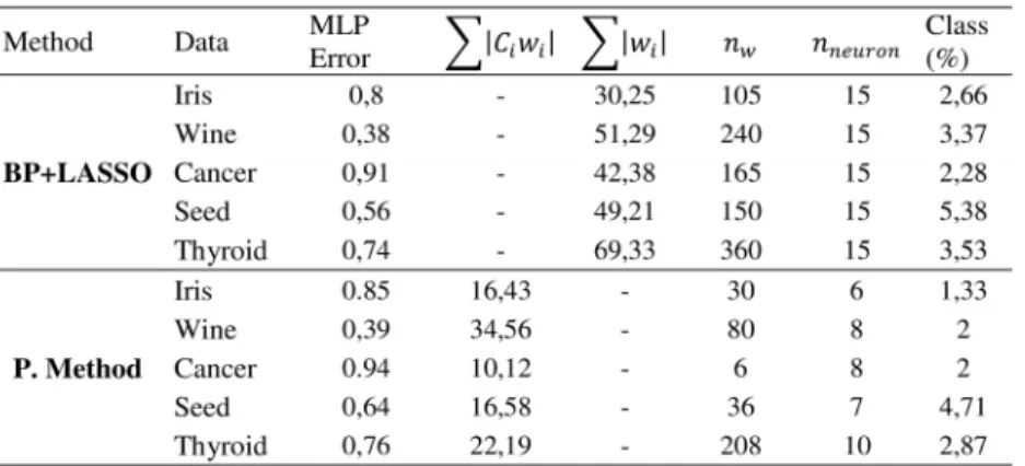
At first, we obtain the right shape of the Pareto front, but it isn’t enough, for our case, the users need only a single solution. It is, from the algorithm point of view, all the solution in the Pareto front are equally important. For this, many approaches was proposed [31]. We have chosen the must adequate solution between the obtained optimal solutions by an approach basing on the crowding distance. The solution obtained is illustrated in table 3.
Table 2. NSGA II Parameter setting
The class presented in table 3 is calculate by the following formula:
The P. Method in table 3 represent the proposed model and BP+LASSO represent the Back propagation method with a regularized error. Well, in order to prove the efficiency of our approach, we compare it to BP+LASSO. The back propagation is applied to minimize the MLP error with a second term, aiming to regulate the current error, the error is presented as:
The β is a parameter fixed by testing several time with different value (0,05; 0,1; 0,15 …), the best results was find at β = 0, 1. Which to presented results in table 3.
From the table 3 we can see that our approach obtain a better results in the regulation term, compared to the BP+LASSO, as we have add a decision variable. The number of the connections and neurons are also considerably reduces compared to the BP+LASSO Method. The table 3, also chows a better calculate class rate for the proposed model. In this fact, we can say that the proposed model is able to provide a good generalization and reduce the MLP topology.
6. Conclusion
In this paper, a new multiobjective learning model is presented to improve the MLPs generalization by minimizing the training error and controlling the weights variation of the network during the learning process in order to prune the network efficiently. Furthermore, we have proposed two new constraints to ensure the communication between connection and neurons. The model was solved by adapting the NSGA II algorithm to the current model.
The results show that the proposed method allow to reduce unnecessary nodes and connections, compared to algorithm that minimize only the regularized error, such as standard backpropagation with Lasso regularizer, our approach was able to reach higher generalization solutions for different Data problems, well as a reduced topology.
References
[1] Rumelhart, D. E., Hinton, G. E., Williams, R. J. (1986). Learning representations by backpropagation error. Nature. 323. 533-536 [2] Ramchoun, H., Janati Idrissi, M A., Ghanou, Y., Ettaouil, M. (2017). New Modeling of Multilayer Perceptron Architecture Optimization with Regularization: An Application to Pattern Classification, IAENG International Journal of Computer Science, 44 (3) 261-269.
[3] Abdelatif, E. S., Fidae, H., Mohamed, E. (2014). Optimization of the Organized KOHONEN Map by a New Model of Preprocess-ing Phase and Application in ClusterPreprocess-ing. Journal of EmergPreprocess-ing Technologies in Web Intelligence. 6 (1) 80-85 (2014).
[4] Arlot, S., Celisse, A. (2010). A survey of cross-validation procedures for model selection. Statistics Surveys. 4, 40-79. [5] Reed, R. (1993). Pruning algorithms-a survey. IEEE Transactions on Neural Networks. 4 (5) 740- 747.
[6] Kwok, T. Y. (1996). Constructive algorithms for structure learning in feedforward neural networks (Doctoral dissertation). [7] Bartlett, P. L. (1997). For valid generalization the size of the weights is more important than the size of the network. In: Advances in neural information processing systems. 134-140.
[8] De Albuquerque Teixeira, R., Braga, A. P., Takahashi, R. H., Saldanha, R. R. (2000). Improving generalization of MLPs with multi-objective optimization. Neurocomputing. 35 (1) 189-194.
[9] De Albuquerque Teixeira, R., Braga, A. P., Takahashi, R. H., Saldanha, R. R. (2001) Recent advances in the MOBJ algorithm for training artificial neural networks. International Journal of Neural systems. 11 (03) 265-270.
[10] Costa, M. A., Braga, A. P. (2006). Optimization of neural networks with multi-objective lasso algorithm. In Neural Networks, (17)
2006. IJCNN’06. International Joint Conference on. IEEE. 3312-3318 (2006, July).
[11] Chankong, V., Haimes, Y. Y. (2008). Multiobjective decision-making: theory and methodology. Courier Dover Publications. [12] Deb, K., Agrawal, S., Pratap, A., Meyarivan, T. (2000). A fast elitist non-dominated sorting genetic algorithm for multi-objective optimization: NSGA-II. In International Conference on Parallel Problem Solving From Nature. Springer, Berlin, Heidel-berg. 849-858 (2000, September).
[13] Liu, G. P., Kadirkamanathan, V. (1995). Learning with multi-objective criteria. In: 4th International Conference on Artificial Neural Networks. 53 – 58.
[14] Costa, M. A., Braga, A. P., Menezes, B. R., Teixeira, R. A., Parma, G. G. (2003). Training neural networks with a multi-objective sliding mode control algorithm. Neurocomputing. 51, 467- 473.
[15] Braga, A., Takahashi, R., Costa, M., Teixeira, R. (2006). objective algorithms for neural networks learning. Multi-objective machine learning, Springer. 151-171.
[16] Costa, M. A., de Pádua Braga, A., de Menezes, B. R. (2007). Improving generalization of MLPs with sliding mode control and the Levenberg–Marquardt algorithm. Neurocomputing. 70 (7), 1342-1347.
[17] Janati Idrissi, M A., Ramchoun, H., Ghanou, Y., Ettaouil, M. (2016). Genetic algorithm for neural network architecture optimi-zation, In: IEEE Proceeding of the 3rd International Conference of Logistics Operations Management 2016. IEEE. Morocco. (2016, 23-25 May). 10
[18] Senhaji, K., Ettaouil, M. (2017). Multi-criteria optimization of neural networks using multiobjective genetic algorithm. In: 2017 Intelligent Systems and Computer Vision (ISCV). IEEE. 4-p (2017, April).
[19] Rosenblatt, F. (1958). The Perceptron, A Theory of Statistical Separability in Cognitive Systems, Cornell Aeronautical Laboratory. Tr. No. VG-1196-6-1 (January).
[20] Ghanou, Y., Bencheikh, G. (2016). Architecture Optimization and Training for the Multilayer Perceptron using Ant System. Architecture. 28, 10.
[21] Salomon, D. (2004). Data compression: the complete reference. Springer Science & Business Media.
[22] Sietsma, J., Dow, R. J. (1991). Creating artificial neural networks that generalize. Neural Networks. 4 (1) 67-79 (1991). [23] Holland, J. H. (1975). Adaptation in natural and artificial systems. An introductory analysis with application to biology, control, and artificial intelligence. Ann Arbor. MI: University of Michigan Press.
[24] Coello, C. A. C., Lamont, G. B., Van Veldhuizen, D. A. (2007). Evolutionary algorithms for solving multi-objective problems. New York. Springer. 5.
[25] Jaimes, A. L., Coello, C. A. C. (2008). An introduction to multi-objective evolutionary algorithms and some of their potential uses in biology. In: Applications of Computational Intelligence in Biology. Springer Berlin Heidelberg. 79-102 (2008).
[26] Srinivas, N., Deb, K. (1994). Muiltiobjective optimization using nondominated sorting in genetic algorithms. Evolutionary Computation. 2 (3) 221-248.
[27] Zitzler, E., Deb, K., Thiele, L. (2000). Comparison of multiobjective evolutionary algorithms: Empirical results. Evolutionary Computation. 8(2) 173-195.
[28] Zitzler, E., Thiele, L. (1998). Multiobjective optimization using evolutionary algorithms-a comparative case study. In: Interna-tional Conference on parallel problem solving from nature. Springer. Berlin. Heidelberg. 292-301 (September).
[29] Jebari, K., Madiafi, M. (2013). Selection methods for genetic algorithms. International Journal of Emerging Sciences. 3 (4) 333-344 .
[30] Hingee, K., Hutter, M. (2008). Equivalence of probabilistic tournament and polynomial ranking selection. In CEC 2008. (IEEE World Congress on Computational Intelligence). IEEE Congress on Evolutionary Computation, IEEE. 564-571 (June).