Corresponding Author: Payam Salimi, Faculty of Industrial and Mechanical Engineering, Islamic Azad University, Qazvin Branch, Qazvin, Iran
E-mail:[email protected]
Cost-Oriented Assembly Line Balancing by Considering Resource Constraint
Payam Salimi, Esmail Mehdizadeh, Behroz Afshar Nadjafi
Faculty of Industrial and Mechanical Engineering, Islamic Azad University, Qazvin Branch, Qazvin,
Iran
Abstract: With today’s trend towards production customization, optimum usage of the available facilities and operators who are able to perform many tasks is of major importance. Usually in classical assembly line balancing problems the tasks are directly assigned to the stations without considering the resources such as machines and proper operators needed to perform that task. However in many realistic situations assigning a task to a station require the existence of some specific resources in that station. On the other hand, considering the high competition among different producers in today’s markets, reducing the costs of production has a major priority for production managers. Considering the gap between the real world assembly line systems and the models considered in the literature of assembly line balancing problems, developing a model that represent the production costs under more realistic situation, as a step towards reducing this gap, is vital. The addressed problem is modeled mathematically and solved by parameter calibrated optimization meta-heuristic algorithms. The performed analysis demonstrates the applicability of the developed model and the algorithms.
Key words: Assembly line; cost-oriented production planning; resource constraints; genetic algorithm; simulated annealing.
Introduction and Literature Review:
Assembly lines are flow-based production systems used to manufacture standardized production units in high volume. These systems even gain importance in manufacturing customized products in low volume. Assembly lines consist of workstations positioned along a conveyor belt or similar material handling system. In each station a set of tasks are performed on the work-piece. Beginning from the first station, each work-piece is moved from station to station with a constant transportation speed throughout the line. The production speed is determined by the cycle time which is the time between completions of two consecutive production units. The work content of each station in the line is constrained to be less than or equal to the cycle time. The total work needed to assemble the final product is divided into n basic operations I= {1, 2… n}, these elementary operations are called tasks. Each task j needs units of time to be accomplished; this duration is called task time. Furthermore there are some precedence relations between tasks. Typically these relations are presented in a precedence graph in which each vertex presents a task and each arc (i,j) presents a precedence relation between tasks i and j.
consider minimizing the total cost of station and task duplications by developing a branch and bound and branch and bound heuristic algorithms.
The resource constraints have not been considered in the cost-oriented approaches of assembly line balancing problems’ literature, while in the real assembly lines they are restriction on labor, workers special ability, tools, machines and etc resources of manufacturing and it does not practically possible to assign tasks to any arbitrary workstation. Resource constrained assembly line problems has lack literature in the class of problem unlike its importance and significant effect on assigning and production planning. In the literature the resource constrained in hardly found except the Ahmadi and Kouvelis, 1999 which considered the resource allocation in an electronic Industry and emphasizes on Mini-Line, Flexible Flow Line, and Hybrid Line designs and the trade-offs associated with these design alternatives, or Miralles et al., 2008 which studied the worker assignment problem. The main study on resource allocation is done by Agpak and Gokcen, 2005, they defined a specific resource for every task, and then by considering the restriction of these resources, the problem of task allocation is solved by a mathematical formulation. Corominas et al., 2011, followed this study and made the resource definition wider. Because of the lack of the subject in cost-oriented area of line balancing problems and the importance of resource constraints and production costs, this paper motivated to consider these issues. The problem description and mathematical modeling is explained in next section.
Problem Description:
In this section the considered problem is defined in detail and the developed model along with the simple small sample is solved by the model to describe the problem easier and more understandable.
The straight un-paced assembly line as defined in previews introduction section, branches in to vary problems depending on the manager demand, line situation and etc as SALBP-I, SALBP-II, SALBP-E and SALBP-F, where in SALBP-I the problem is to optimizing the number of workstations by proper tasks assignment knowing the cycle time. SALBP-II considers the cycle time minimization by determined exact number of workstations. SALBP-E is seeks the solution which gives best efficiency of line by using the maximum capacity of the cycle time in all stations. And SALBP-F is just considers the feasible solutions of tasks assignment in a determined cycle time and station number assembly line. The main base and assumptions of this kind of assembly line can be described as follows:
The assembly line is in a straight manner including several following stations separated by buffers. • Only one task is done at the same time in each station.
• The line produces single product in each cycle.
• Machine breakdowns and product decay are not considered.
• As considering the precedence relations, the successor tasks are not assigned to former stations. • The tasks times are deterministic
• According to the type of SALBP, the number of stations is deterministic (SALBP-II) or the cycle time is predetermined (SALBP-I)
This paper considers the cost-oriented, resource consideration problem under the SALBP-I framework, where workstation creation costs, operator wages, product costs and etc, are considered while dealing with resource restrictions and costs. The main assumptions and the framework of this study are as follows:
• Tasks times are deterministic, but may vary depending on the resource it uses. • Each task needs one resource to be done in a station.
• It may be several possible resources to do the task, but only one of them is allocated to specific task. • Since each of resources takes some place in the station, the number of resources limits by the total size of
the station.
The details of cost-oriented line are illustrated along with model presentation. Modeling:
In this section the whole model with all assumptions of costs and resource restrictions are described under the SALBP-I construction. For this aim the all parameters and variables needed to define the model is presented as follows:
Sets:
I The set of all tasks
IPi The Set of predecessors of tasks i
R The set of all resources
Ri The set of resources possible to do task i
Ir The set of tasks that can be done by resource r
Indexes and Parameters:
i,h Indicate tasks
k,j Indicates stations
R Indicates resources
N Number of All Tasks
R Number of All Resources
Mmax The maximum number of stations
The space needed by resource r tir Task i process time if resource r is used
C Cycle time
A Total size of each station RCr The cost of resource r
The wage rate for task i The wage rate for station j The investment cost per station Variables:
Z The integer number of active stations (Z≤Mmax)
1 if task i performs in station j by using resource r, otherwise 0 1 if resource r used in station j, otherwise 0
The cost of operator wages depends on the task value, which determined by considering the difficulty of the task and described by , where MU is Monetary Unit and TU is Time Unit. The wage of the operator in a station is defined by means of the most difficult task (the most valuable), and so the wage of the whole station
is: . And so the total wage is described as: .
On the other hand the cost of work piece traveling through the stations depends on the length of the line which depends on the number of stations and assumed as and the total of this type of cost is calculated as . At the end the cost of used resource is assumed as .
The objective of the problem is to optimize the costs of the line by considering the restrictions of resources. And the mathematical formulation is developed as:
Mathematical Formulation:
1
Subject to:
2
3
4
5
6
7
Equation (1) shows the objective function which includes the station investment costs, operator costs and the resource costs, respectively. Constraint (2) describes that every task should be done in one station by single resource. Constraint (3) describes the station wage which determined by the maximum operator wage in station. And inequality (4) shows the precedence relation. Cycle time limitation is shown by (5). Constraint (6) determines the usage of resources in stations. Constraint (7) limits the resource allocations to a station by considering the total station size and the size needed by resources. And finally inequality (8) presents the number of active stations.
Numerical Small Example:
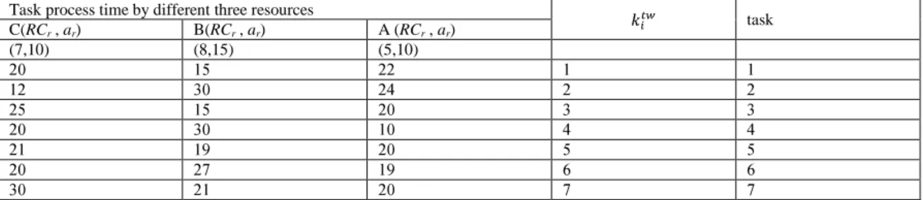
In this section one small example with 7 tasks and 3 resources presented to better illustrate the model. The cycle time is assumed as 45 and the station size is 20 units, and also the investment cost of each station assumed as 20 money units. The precedence relations graph of this problem is portrayed in Figure.1. The all needed input data is given in Table.1 which presents the tasks times of tasks in three A, B and C resources conditions, wage rates, resource costs and the resource needed size.
The problem with the above details is solved by CPLEX and the results shown in Table.2. This Table shows the assigned tasks, number of workstations, used resources by tasks and station wage. By means of these results, the rest of costs are calculable.
The tasks 1,2,4 are assigned to first station using resources A and C and by the total station wage of 4, by considering the limitation of cycle time, tasks 3 and 5 are assigned to new opened second station using resource A and by the total station wage of 5, and the end by opening the third workstation, tasks 6 and 7 are assigned using resource A and the total station wage of 7. The rest of the costs can be calculated by means of these results.
Fig. 1: Precedence relations of example with 7 tasks.
Table 1: Input data for problem with 7 tasks.
task Task process time by different three resources
A (RCr , ar) B(RCr , ar)
C(RCr , ar)
(5,10) (8,15)
(7,10)
Since the optimal number of stations resulted 3, so the station investment costs is 60 (3×20), the total stations wages is 16(4+5+7), operators wages is 720 and the resource costs is 26. So the total cost of a product is 806.
Table 2: Results of problem with 7 tasks.
Station wage Used Resource
Task Assignment Station
4 A,C
1,2,4 1
5 A
3,5 2
7 A
6,7 3
Problem Complexity:
Meta-heuristic Algorithms: Genetic Algorithm:
Genetic algorithm (GA) is a robust algorithm for optimization problems. In a simple GA, at first, a population of the feasible solutions is produced through a random process; afterwards, a fitness value is calculated for each solution in the population, then solutions are ranked based on their fitness values. Next, on the basis of a selection mechanism, a set of chromosomes is chosen to perform the crossover and mutation. This process is called generation; the generation is iterated until the stopping conditions be met. Also extend application in the assembly line balancing problems (see for example Kim et al., 1997, Chen et al., 2002, Tasan and Tunali, 2008, Kim et al., 2009, Raghda et al., 2011,Akpinar and Bayhan, 2011, Rajabalipour et al., 2012, Palencia and Delgadillo, 2012, Mutlu et al., 2013, Purnomo et al., 2013).
Encoding:
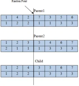
The chromosome of the GA is designed in two rows, which the first row shows the performance priority of tasks and the second row determines the resource used by the task. The sample of this chromosome type for the presented small example with 7 tasks is shown in Figure. 2. It is obvious that the in first row the tasks permutation follows the precedence relations.
Fig. 2: Chromosome Sample. Fitness Function:
Based on the produced chromosome for every population members, fitness function calculated according to the costs relevant to the produced assignments of tasks and resources. The aim of the algorithm is to minimize this function.
Selection and Replacement:
In this developed GA, Roulette wheel (Sivanandam and Deepa, 2008) selection method is applied, which gives more chance for the chromosomes (Solutions) with better fitness function to be selected as base chromosomes to do crossover and mutation.
Also another elitism procedure is applied as replacement, which selects best 10 percent of the current population and moves them to next population.
Crossover:
The crossover operator takes two selected chromosomes by the Roulette wheel method as parents and combines some characteristics of them to produce a new child (chromosome). This operator is done with hope to produce better solutions.
In this paper the OX crossover methodology is applied which is proper to the chromosomes that should observe the precedence relations. The crossover operator should perform on both the first and second row of the chromosome, separately.
At first a random point on first row is selected and divides the both first chromosome (parent 1) and second chromosome (parent 2) in to right and left part. Then the new child inherits the left side genomes (tasks) from first parent and observes the order of these genomes from second parent. Then the child inherits the right side from the right side of first parent by observing the second parents' order.
The second child’s first row is also produced by the same procedure. The second row of first child is produced as similar as the first row, but the child inherits the left side as same as in first parent, and its right side from the second parent.
Mutation:
The mutation operator performs in order to prevent the results trapping in local optimum. For the first row randomly selected genome exchange its place by beside right genome considering the precedence relation. For the second row, just two randomly selected genomes exchange their places.
Restart Scheme:
In this paper an additional operator is performed in order to expand the population diversity (Vallada and Ruiz, 2010, Ruiz et al., 2005, Bahalke et al., 2010). The procedure is performed if the best gained solution does not change for following Griterations. The application steps ar as follows:
1. Count=0;
2. In iteration i , Costi=best answer(minimum fitness function);
4. If (Count>Gr)
5. Sort the population from best to worse fitness function. 6. Directly transfer the 20 percent best results to new population.
7. 50 percent of new population is generated by doing mutations on first 20 percent. 8. Rest 30 percent is produced randomly.
Fig. 3: Crossover. Simulated Annealing:
Simulated annealing (SA) is a generi locating a good approximation to the global optimum of a given function in a large search space. It is often used when the search space is discrete (e.g., all tours that visit a given set of cities).
SA starts with a initial solution, the produces new neighborhood solution, the new solution is accepted to exchange with current solution under the following probability conditions.
It tells that if the current solution be worse than the new solution’s fitness function ( ), the new one is substituted by current one or if the current solution be better than new one, it also has the chance to substitute by current solution. Unlike to the other generic optimization algorithms, SA also gives chance to new worse solutions. This performance expands the solution diversity. T is a deterministic parameter.
Initial Solution:
In this paper the initial solution is created by random process by observing the precedence graph. Neighborhood Creation:
There are two designed procedures to create the feasible solution which each of them is selected by half probability. The first one is exactly as the mutation process in GA and the second one which emphasizes on resources selects a random genome and assigns a random resource to that specific task.
Diversity Expanse Scheme:
A scheme is designed to prevent the solutions from trapping in local optimum. It is similar to the restart scheme in GA, while in SA the scheme starts when the best result does not improve for dn following iterations. It produces 200 neighborhoods for current solution, and then the best answer of these 200 different solutions is substituted by the current solution.
Cooling:
The cooling operation in this SA follows the formulation, while is the temperature in iteration
i and q is cooling rate. Computational Results:
most effective parameters among the existing levels of factors. There are numerous methods for designing the experiments to identify the significant relation between the various factors affecting the output of a process. Parameter Calibration of GA:
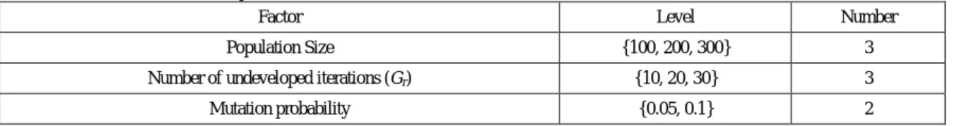
The factors and levels of the developed GA are presented in Table.3, which includes of factors population size, the number of iteration parameter for the restart scheme and mutation probability. Three levels of 100, 200 and 300 are proposed for the population size, three levels of 10, 20 and 30 are proposed for parameter Gr and two levels of 0.05 and 0.1 for the mutation probability.
Table 3: Factors and levels for GA parameters.
Factor Level Number
Population Size {100, 200, 300} 3
Number of undeveloped iterations (Gr) {10, 20, 30} 3
Mutation probability {0.05, 0.1} 2
Since the number of all combinations for the above case is 18 (3×3×2), then it is better to perform the full factorial one. The experiments are done for the three sizes of the problem (small, medium and large sizes). Small Size:
The problem with 20 tasks and 6 resources is considered. The results of full factorial design are presented in Table.4 and Figure 4.
Table 4:The experiment result for problem with 20 tasks and 6 resources.
Source DF Seq SS Adj SS Adj MS F P
POP-Size 2 1.261 1.261 0.6305 1.43 0.34
Gr 2 0.0532 0.0532 0.0266 0.06 0.942
mut_prob 1 4.9458 4.9458 4.9458 11.2 0.029
pop_size×GR 4 2.1713 2.1713 0.5428 1.23 0.423
pop_size×mut_prob 2 1.8192 1.8192 0.9096 2.06 0.243
Gr×mut_prob 2 2.3037 2.3037 1.1518 2.61 0.188
Error 4 1.7658 1.7658 0.4415
Total 17 14.32
In the DOE method the main effective factors identified by P value, it means that if the value of P value be less than 1-α, that factor is identified as effective factor, where α is the confident level (95% in this paper). Thus the results in Table.4 show that the mutation probability factor is the most effective factor among the others. For choosing the best levels of the factors the main effect plot is presented in Figure 4 by means of the Minitab statistical software. It shows that the in population size of 100 the results are better, 30 is better for Gr and 0.1 is better for mutation probability. By this trend the results achieved for the medium and large size problems in following Tables and Figures. The Table 7 shows the final best identified levels for all three sizes of the problems.
Fig. 4: Levels effects comparison for the problem with 20 tasks and 6 resources. 3
2 1
9.50 9.25 9.00 8.75
8.50
3 2
1
2 1
9.50 9.25 9.00 8.75 8.50
pop_size
M
ea
n
GR
mut_prob
Main Effects Plot for res
Medium Size:
The problem with 50 tasks and 10 resources is considered as the medium size example for the experiments.
Table 5:The experiment result for problem with 50 tasks and 10 resources.
Source DF Seq SS Adj SS Adj MS F P
pop_size 2 58.3108 58.3108 29.1554 34.75 0.003
GR 2 0.1943 0.1943 0.0972 0.12 0.894
mut_prob 1 0.0035 0.0035 0.0035 0 0.952
pop_size×GR 4 0.422 0.422 0.1055 0.13 0.965
pop_size×mut_prob 2 0.1627 0.1627 0.0814 0.1 0.91
GR×mut_prob 2 1.5 1.5 0.75 0.89 0.478
Error 4 3.3563 3.3563 0.8391
Total 17 63.9497
The main plot for this medium size example is presented in Figure 5 as follows.
Fig. 5: Main effect plot for the problem with 50 tasks and 10 resources. Large Size:
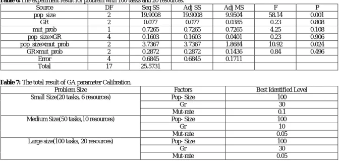
The problem with 100 tasks and 20 resources is considered as large size experiment and the results are presented in Table 6 and Figure 6.
Table 6:The experiment result for problem with 100 tasks and 20 resources.
Source DF Seq SS Adj SS Adj MS F P
pop_size 2 19.9008 19.9008 9.9504 58.14 0.001
GR 2 0.077 0.077 0.0385 0.23 0.808
mut_prob 1 0.7265 0.7265 0.7265 4.25 0.108
pop_size×GR 4 0.1603 0.1603 0.0401 0.23 0.906
pop_size×mut_prob 2 3.7367 3.7367 1.8684 10.92 0.024
GR×mut_prob 2 0.2872 0.2872 0.1436 0.84 0.496
Error 4 0.6845 0.6845 0.1711
Total 17 25.5731
Table 7: The total result of GA parameter Calibration.
Problem Size Factors Best Identified Level
Small Size(20 tasks, 6 resources) Pop- Size 100
Gr 30
Mut-rate 0.1
Medium Size(50 tasks,10 resources) Pop- Size 100
Gr 10
Mut-rate 0.05
Large size(100 tasks, 20 resources) Pop- Size 100
Gr 30
Mut-rate 0.05
3 2
1 7 6 5 4 3
3 2
1
2 1
7 6 5
4 3
pop_size
M
ea
n
GR
mut_prob
Main Effects Plot for res
Fig. 6: Main effect plot for the problem with 50 tasks and 10 resources. Parameter Calibration of SA:
As similar as previews section the calibration of parameters for SA algorithm is done and for the parameters and factors considered in Table. 8, the best identified parameters of SA for the three sizes of problems are presented in Table.9.
Table 8: Factors and Levels for the SA parameters.
Factor Level Number
Initial Tempreture(init_Temp) {100, 150, 350} 3
Cooling rate(CL) {0.7, 0.8, 0.9} 3
Number of iteration in each temreture(Nit) {50, 100, 150} 3
The number of iteration for diversity expanse scheme(dn) {50, 100} 2
Table 9: The result of Calibration of SA parameters.
Problem Size Factors Best Identified Level
Small Size(20 tasks, 6 resources) init_Temp 350
CL 0.8
Nit 150
Dn 100
Medium Size(50 tasks,10 resources) init_Temp 350
CL 0.9
Nit 150
Dn 100
Large size(100 tasks, 20 resources) init_Temp 150
CL 0.7
Nit 50
Dn 100
Problem Solving:
In this section three sizes of problems extracted from the data base collected in www.assembly-line-balancing.de are considered and solved by the developed model and algorithms.
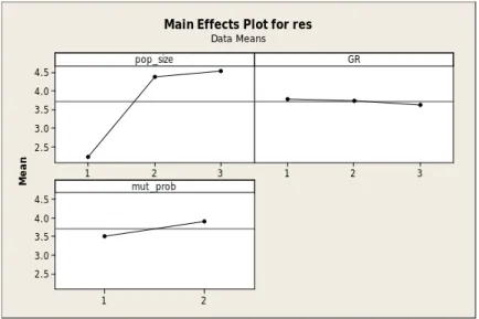
Small Size:
Three small examples of BOWMAN with 8 tasks, JAESCHKE with 9 tasks and JACKSON with 11 tasks are considered for this section. The problems solved by mathematical model, GA and SA. The assumed resources and other data are presented in Table 10.
For above problems GA and SA are runed 5 times and the terminal condition to stop the algorithms is set to 30 seconds. The means and standard deviations are also presented in results in Table 11. The results of this table show that the algorithms resulted in optimal solutions without any deviation for all three examples, however it is seen that the running time for both algorithms are nearly zero.
3 2
1 4.5 4.0 3.5 3.0 2.5
3 2
1
2 1
4.5 4.0 3.5 3.0 2.5
pop_size
M
ea
n
GR
mut_prob
Main Effects Plot for res
Table 10: Data for the three small examples.
Tasks 1 2 3 4 5 6 7 8 Problem
Resource1/tij 5 14 9 15 8 14 15 20 BOWMAN
Resource2/tij 19 5 10 20 20 5 9 6
Resource3/tij 7 16 20 8 9 13 8 13
8 18 15 11 15 9 11 8
Tasks 1 2 3 4 5 6 7 8 9 JAESCHKE
Resource1/tij 9 15 7 12 10 10 16 16 16
Resource2/tij 13 17 6 12 15 18 20 8 7
Resource3/tij 12 10 17 5 6 16 11 11 18
13 14 10 9 5 9 5 10 17
Tasks 1 2 3 4 5 6 7 8 9 10 11 JACKSON
Resource1/tij 9 9 7 16 8 15 14 8 17 13 17
Resource2/tij 19 17 10 16 9 9 5 18 7 5 11
Resource3/tij 6 20 10 10 9 7 8 19 20 17 17
8 20 8 14 7 15 16 18 12 18 18
Table 11: Final Results for the Small Size examples.
Solution methodology
Problem model
GA SA
time result
Mean time Mean
result SD time
SD result Mean
time Mean result SD time
SD result
BOWMAN 3.34
0.0001 0.00001
0.006 0.003
JAESCHKE 5.56
0.0007 0.0002
0.004 0.002
JACKSON 11.12
0.007 0.001
0.008 0.004
Medium Size:
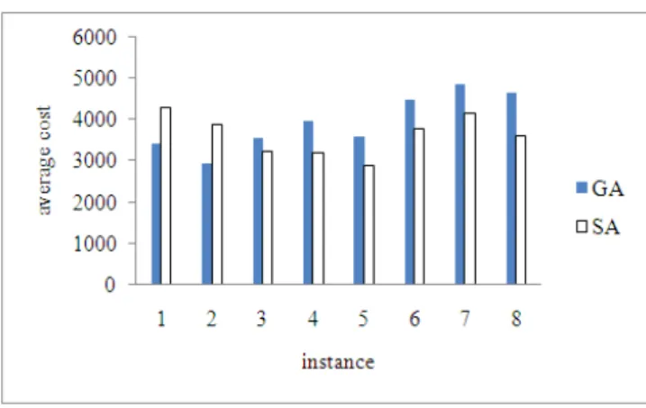
In this section the 8 problems with the 20 to 30 tasks and with 5 to 15 resources are considered and solved by both algorithms. It should be noted that the mathematical model could not solve the problems in this size at a reasonable time. The termination criteria are considered 30 seconds for both algorithms. The results portrayed in Table 12 and figures 7 and 8.
Table 12: Results for medium size problems.
Solution Algorithm Problem
SA GA
SD Mean
SD Mean
No. of resources No. of Tasks
The results of this Table shows that the one single algorithm has not complete domination for another one. This condition is presented in figures 7 and 8. Figure 7 shows the comparisons of two algorithms in the case of mean of results and figure 8 notes the different in the case of standard deviation.
Fig. 8: SA and GA comparision in the case of mean of the result for the medium size problems.
Figure 7 shows that for the fisrt and second medium size problems, GA have the better mean of total costs, but for the rest of problems solved better with SA algorithm. The figure 8 demonstraits that GA has better standard deviation than SA, exept in fifth and eighth problems.
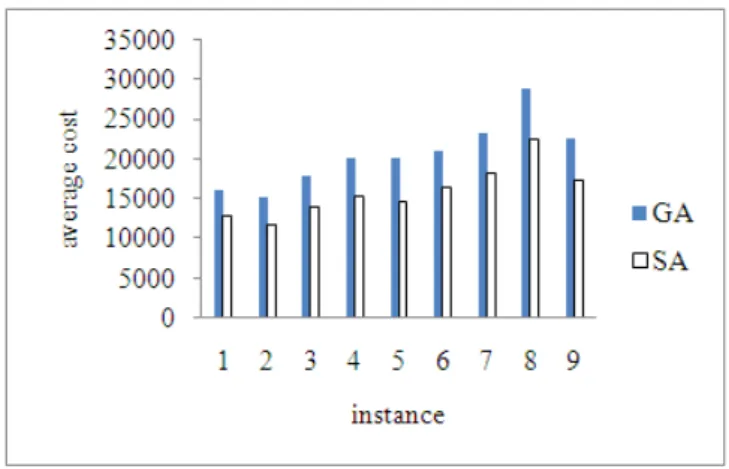
Large Size:
In this section 9 examples with 100 to 140 tasks and 20 to 50 resources are considered and solved by SA and GA algorithms. The results concluded in Table 13.
Table 13: Total Results of large size problems.
Solution Algorithm Problem
SA GA
SD Mean
SD Mean
No. of resources No. of Tasks
The above Table shows the complete dominance of SA for GA in the case of mean of the costs it achieved. This fact is touchable in figure 9, which in the all problems SA has better mean result than GA.
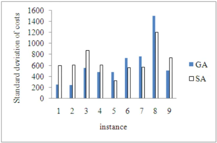
Fig. 9: SA and GA comparision in the case of mean of the results for the large size problems.
Fig. 10: SA and GA comparision in the case of standard deviation of the results for the large size problems. SA and GA Comparison:
In this section the Statistical hypothesis testing is done to find out the difference of two algorithms more accurately. For this aim the Null- hypothesis and Alternative- hypothesis ae considered as follows:
By means of the simple ANOVA the results came out considering confintial rate as 95% shown in Table.14.
Table 14: The result of camparisons of mean costs resulted by SA and GA.
Experiment result p-value
t Problem size
Accept Null Hypothesis Acquittal Medium
Reject Null Hypothesis Conviction Large
Conclusions and Future Research:
In this paper the problem of Simple Assembly Line Balancing is considered under the todays most concerns of facilities, which relates to the production constraints and commodities costs in production plants. In almost all of the realistic situations, assigning a task to a station require the existence of some specific resources in that station. On the other hand, considering the high competition among different producers in today’s markets, reducing the costs of production has a major priority for production managers. This paper considers the resource allocation restrictions and their costs in a cost oriented assembly line problem which the costs of satations, investments, resources, operator and station wages depending on type of tasks are all considered with aim of minimizing the costs along with number of stations. The addressed problem is modeled mathematically and solved by parameter calibrated optimization meta-heuristic algorithms. The performed analysis and results demonstrates the capability of both algorithms, and the comparsons show that the Developed calibrated SA have better results than the presented GA in large range of the problems.
For the future research this paper proposes the considering these costs and more realistic constraints in new versions of line types and also improving, developing and adabting of existence heuristics in problem branch to the addressed problem is highly recommended.
REFERENCES
Agpak, K., H. Gokcen, 2005. 'Assembly line balancing: Two resource constrained cases' , International journal of production economics, 96: 129-140.
Ahmadi, R., P. Kouvelis, 1999.
European Journal of Operational Research, 115(1): 113-137.
Ahmadi, R.H., S. Dasu, C.S. Tang, 1992. 'The dynamic line allocation problem' Management Science, 38: 1341-1353.
algorithm for mixed-model assembly line balancing problem with sequence dependent setup times between
Engineering Applications of Artificial Intelligence,
24(3): 449-457.
Amen, M., 2000. ‘An exact method for cost-oriented assembly line balancing Original Research Article’
International Journal of Production Economic’s, 64(1-3): 187-195.
Bahalke, U., A.M. Yolmeh, K. Shahanaghi, 2010. 'Meta-heuristics to solve single-machine scheduling problem with sequence-dependent setup time and deteriorating jobs' Int J Adv Manuf Technol, 50: 749-759.
Baker, K.R., S.G. Powell, D.F. Pyke, 1990. 'Buffered and unbuffered assembly systems with variable processing times' Journal of Manufacturing and Operations Management, 3: 200-223.
Becker, C., A. Scholl, 2009. ‘Balancing assembly lines with variable parallel workplaces: Problem definition and effective solution procedure European Journal of Operational Research, 199(2): 359-374.
Betul Yagmahan, 2011. ‘Mixed-model assembly line balancing using a multi-objective ant colony optimization approach’ Expert Systems with Applications, 38(10): 12453-12461.
Boysen, N., M. Fliedner, A. Scholl, 2009. ‘Sequencing mixed-model assembly lines: Survey, classification and model critique’, European Journal of Operational Research, 192(2): 349-373.
Bukchin, Y., I. Rabinowitch, 2006. ‘ A branch-and-bound based solution approach for the mixed-model assembly line-balancing problem for minimizing stations and task duplication costs’ European Journal of Operational Research, 174(1): 492-508.
Buzacott, J.A., 1968. 'Prediction of the efficiency of production systems without internal storage'
International Journal of Production Research, 6: 173-188.
Chen, R.S., K.Y. Lu, S.C. Yu, 2002. ‘A hybrid genetic algorithm approach on multi-objective of assembly planning problem’. Engineering Applications of Artificial Intelligence, 15: 447-457.
Cheshmehgaz, H.R., H. Haron, F. Kazemipour, M.I. Desa, 2012. ‘Accumulated risk of body postures in assembly line balancing problem and modeling through a multi-criteria fuzzy-genetic algorithm’, Computers & Industrial Engineering, 63(2): 503-512.
Deckro, R.F., 1989. 'Balancing cycle time and workstations' IIE Transactions, 21: 106-111.
Dolgui, A., A. Ereemev, A. Kolokolov, V. Sigaev, 2002. 'A genetic algorithm for allocation of buffer storage capacities in production line with unreliable machines' Journal of Mathematical Modelling and Algorithms, 1: 89-104.
Globerson, S., A. Tamir, 1980. 'The relationship between job design, human behavior and system response'
International Journal of Production Research, 18: 391-400.
Hamzadayi, A., G. Yildiz, 2012. ‘A genetic algorithm based approach for simultaneously balancing and sequencing of mixed-model U-lines with parallel workstations and zoning constraints’, Computers & Industrial Engineering, 62(1): 206-215.
Hillier, F.S., K.C. So, 1991. 'The effect of machine breakdowns and interstage storage on the performance of production line systems' International Journal of Production Research, 29: 2043-2055.
Hillier, F.S., K.C. So, R.W. Boling, 1993. 'Toward characterizing the optimal allocation of storage space in production line systems with variable processing times' Management Science, 39: 126-133.
Kim, Y.J., Y.K. Kim, Y. Cho, 1997. ‘A heuristic-based genetic algorithm for workload smoothing in assembly lines’. Computers & Operations Research, 25: 99-111.
Kim, Y.K., W.S. Song, J.H. Kim, 2009. ‘A mathematical model and a genetic algorithm for two-sided assembly line balancing’. Computers & Operations Research, 36: 853-865.
Malakooti, B., 1994. 'Assembly line balancing with buffers by multiple criteria optimization' International Journal of Production Research, 32: 2159-2178.
Manavizadeh, N., M. Rabbani, D. Moshtaghi, F. Jolai, 2012. ‘Mixed-model assembly line balancing in the make-to-order and stochastic environment using multi-objective evolutionary algorithms’, Expert Systems with Applications, 39(15): 12026-12031.
Miltenburg, J., J. Wijngaard, 1994. 'The U–line line balancing problem' Management Science, 40: 1378-1388.
Miralles, C., J. García-Sabate, C. Andrés, M. Cardós, 2008. ‘Branch and bound procedures for solving the Assembly Line Worker Assignment and Balancing Problem: Application to Sheltered Work centres for Disabled’, Discrete Applied Mathematics, 156(3): 352-367.
Monden, Y., 1998. Toyota production system-An integrated approach to just-in-time, Kluwer, Dordrecht. Mutlu, O., O. Polat, A. Supciller, 2013. ‘An iterative genetic algorithm for the assembly line worker assignment and balancing problem of type-II’ Computers & Operations Research, 40(1): 418-426.
Ozbakir, L., A. Baykasoglu, B. Gorkemli, L. Gorkemli, 2011. ‘Multiple-colony ant algorithm for parallel assembly line balancing problem’, Applied Soft Computing, 3: 3186-3198.
Powell, S.G., 1994. 'Buffer allocation in unbalanced threestation serial lines' International Journal of Production Research, 32: 2201-2217.
Purnomo, H.D., H.M. Wee, H. Rau, 2013. ‘Two-sided assembly lines balancing with assignment restrictions’. Mathematical and Computer Modelling, 57(1-2): 189-199.
Rosenberg, O., H. Ziegler, 1992. 'A comparison of heuristic algorithms for cost-oriented assembly line balancing' Zeitschrift fu r Operations Research, 36: 477-495.
Ruiz, R., C. Maroto, J. Alcaraz, 2005. 'Solving the flowshop scheduling problem with sequence-dependent setup times using advanced metaheuristics' Eur J Oper Res., 165: 34-54.
Sivanandam, S.N., S.N. Deepa, 2008. ‘Introduction to genetic algorithms’. Springer, New York, pp: 47-54. Suhail, A., 1983. 'Reliability and optimization considerations in a conveyor-paced assembly line system'
International Journal of Production Research, 21: 627-640.
Taha, R.B., A.K. El-Kharbotly, U.M. Sadek, N.H. Afia, 2011. ‘A Genetic Algorithm for solving two-sided assembly line balancing problems’, Ain Shams Engineering Journal, 2(3-4): 227-240.
Tasan, S.O., S. Tunali, 2008. ‘A review of the current applications of genetic algorithms in assembly line balancing’. Journal of Intelligent Manufacturing, 19: 49-69.