1
A CA Model for Visual Perception Based On Anatomical
Connections
Author names and affiliations
1)Maryam Beigzadeh, Complex Systems and Cybernetic Control Lab, Faculty of Biomedical Engineering, Amirkabir University of Technology (Tehran Poly-Technique). Postal Address: 424 Hafez Ave, Tehran, Iran, 15875-4413.
Email: [email protected] Tel: +98 21 6454 2351
2)Seyyed Mohammad Reza Hashemi Golpayegani *1, Complex Systems and Cybernetic Control Lab, Faculty of Biomedical Engineering, Amirkabir University of Technology (Tehran Poly-Technique).
Postal Address: 424 Hafez Ave, Tehran, Iran, 15875-4413. Tel: +98 21 64542370,
Email: [email protected]
1 *Corresponding Author
2
A CA Model for Visual Perception Based On Anatomical
Connections
Abstract
A phenomenological model of visual perceptual dynamics is proposed based upon the cellular automata (CA) which considers the anatomical connections between visual areas of the macaque brain. Some other important characteristics of neural networks of the brain are also included in the model, such as the excitatory-inhibitory ratio of neural populations, synaptic delays, etc. A new form of “geometric mean interaction rules” among neural populations are also introduced which could be considered more realistic than the previous “arithmetic mean-based rules”. This computational model is capable of showing interesting dynamical behaviors, seen in the visual perceptual states of the brain.
Keywords
Cellular Automata, Visual Perception, Coupled Logistic Maps, Netlets, Brain Networks Connections.
1. Introduction
The exploration to understand and somehow control biological systems, using fundamentals from physics and mathematics has a long history [1]. Among biological systems, the mammalian brain, because of its vastly complex structure and its perfect and stable function, has attracted a special attention. Researchers try to mainly understand and
3
mimic some behavioral and dynamical aspects of the brain, by some appropriate computational model [1].
A cellular automaton (CA) is a mathematical tool to model the systems with many simple elements working together and creating a global evolutionary pattern of behavior [2]. The CA, firstly introduced by Stanislaw Ulam and John von Neumann in 1940s, became more systematically studied by Stephen Wolfram in 1980s. A classic CA is created from cells, each of them is in one of the predefined discrete possible states (e.g. 0 and 1) in each evolutionary time step. Cells take effect from a pre-defined neighborhood around them and could change their initial state into the next state based upon an “interaction rule” with respect to their neighborhood. Today more generalized versions of the CA are being popular , such as probabilistic CA, continuous CA, CA with dynamic rules, etc [3]. Employing CA in the field of neuroscience has shown successful results in the interpretation of some cognitive aspects of the brain [4] [5], [6], [7] [8]. Compared to other computational models such as Artificial Neural Networks (ANN), Spiking Neural Networks (SNN), Coupled Neural Networks (CNNs) and Globally Coupled Maps (GCM), a cellular automaton could be considered as a more general form since it is capable to have properties of all above-mentioned approaches.
We have proposed before that an appropriate form of CA could be used in modeling the visual perceptual dynamics [9]. In this letter we show that by considering the real anatomical connections among the brain networks and using it carefully in the structure of the CA, it could be a well representative model for visual perception, both structurally and dynamically.
4
It has already been demonstrated that brain dynamics (which are reflected in EEG, MEG and ECoG signals) are inherently chaotic [10]. As we perceive different sensory information (i.e. scenes, sounds, odors, etc.) and recognize different patterns, these dynamical processes tend to turn into a more regular pattern. This stage has been referred by other researchers as: “the transients between gas-like randomness and liquid-like order [11]”. According to such paradigm, each stimulus would tend to lead the system to its own “liquid-like attractor” which is different from the other one. Therefore, after the sensorial stimuli, the brain dynamics would start a search in its general chaotic basin of attraction and finally release into its appropriate attractor and recognize that special stimulus. The proposed computational model tries to maintain these attractors and show the possibility of dynamical transitions between them, by changing the parameter values of the model, or the initial condition.
The most important property of CA in modeling complex multi-agent systems is its ability to imitate the “interaction” between those agents to some extent. It means that in the CA we are able to define and adjust different (mostly simple) interaction rules among the agents. This way, we can make any of the agents to “bifurcate” and change patterns of behavior. Interactions among the neural networks of the brain may result into many perceptual, cognitive and motor behaviors.
Connectivity plays an important role in large networked dynamical systems [1]. That is why in biological systems (such as brain networks) the structural (anatomical) and the functional connectivity patterns are being studied with great interest [12] [13] [14] [15]. In modeling approaches, we should firstly determine the connection pattern and relationships between the elements and then define how these –anatomically /
5
functionally- connected networks could make the dynamical behavior of each element and the whole network to evolve in time. In this work we adopt the real anatomical connection matrix in the macaque visual system for our modeling (The work published by Felleman and Essen [16]).
The remainder of this paper is organized as follows: in section 2 we will introduce our proposed model completely. The main structure of the network and its elements are illustrated in section 2.1, and then in sections 2.2 through 2.4, more details are discussed which include: In-layer and between-layer connections, interaction rules of the CA, and finally the way of considering delays in the network.
Section 3 contains the numerical results and simulations of the model. The numerical studies are based on presenting the time series, phase portraits and bifurcation diagrams, frequency content and synchronization patterns of the network, in different conditions mimicking the visual perceptual dynamics. Finally in section 4 we will have the conclusion and more discussions about the whole letter.
2. Proposed Model
In this section we introduce our model of visual perception using anatomical connectivity matrix, on a cellular automaton platform. This model tries to mimic the dynamical behaviors that happen during visual perceptual states. As mentioned before, we are going to use an anatomical connectivity matrix of the macaque visual cortex in our modeling, which has been extracted from the very interesting study of Essen and Felleman [16]. The results of their study on macaque visual cortex was a 35*35 connection matrix (see Appendix A) corresponding to different cortical areas in the occipital, temporal, parietal
6
and frontal cortex of the macaque. This 35*35 connection matrix was then modified into a simpler 30*30 one by Sporns2 [17] (in which the uncertain and not-connected pathways has been omitted). In the new modified and simplified connection matrix, each element could be equal to 0 or 1. Zero values denote a “no-connection” situation, and non–zero ones corresponds to a valid connection between two nodes. This connection matrix is shown to have the “small world” properties which is necessary for the brain to show many of its functional properties such as synchronization [18].
The building blocks of our model are chosen to be a well-known dynamical model: the logistic map (equation (1)), in order to represent “netlets” (populations of 100-1000 excitatory and inhibitory neurons). Netlets were introduced by Hrath in 1970 to describe the activation of an excitatory-inhibitory population of neurons in the cortex [19] [20]. Later, this concept was used in a computational model for visual cortex by Pashaie et.al. [21]. In their approach, each netlet is supposed to work as a complex processing element (CPE) which is modeled by the logistic map:
( ) ( ) ( ( ))) (1)
The reason for using logistic map as the model of a netlet’s dynamics is discussed here. It is shown that the expectation value of netlet activity could be modeled by equation (2) [19] [20]:
( ) ( )∑
( )
[ ( ) ] ∑ [ ( ) ]
(2)
7
In this formulation, is the activation of an isolated netlet at time step , and is its expected value at time step . Parameter stands for the fraction of inhibitory neurons in the netlet, ( ) is the average number of neurons in the netlet with afferent connections from a given excitatory (inhibitory) neuron in the netlet. Parameter is the minimum number of excitatory and inhibitory inputs necessary to trigger a neuron which has received inhibitory inputs, and finally is the total number of inhibitory connections [21].
Graphs of versus for a netlet with the same amount of excitatory and inhibitory connections and is shown in Figure 1-a. it can be seen that the shapes of these curves could be considered very similar to the plots of a modified version of the well-known logistic map (Figure 1-b).
(a) (b)
Figure 1: (a) Fraction of active nodes of a netlet, with the same amount of excitatory and inhibitory connections, at the moment as a function of active nodes at the previous moment. Different curves correspond to different numbers of presynaptic spikes that are necessary to elicit a postsynaptic spike. (b) Group of quadratic functions employed in the generation of the logistic map (in the form of ( )). The curves in this figure are quadratic functions that are plotted for different values assigned to the bifurcation parameter [21].
8
2.1.The main structure of the network and its elements
Based on the anatomical connections described before, our model is considered to have 30 layers, each corresponds to one of the areas in the occipital, temporal, parietal and frontal cortex (in summary, in the visual system) of the macaque brain (see Appendix A). There are N dynamical agents corresponding to N netlets in each layer. The generalized form of coupled logistic maps would be:
( ) ( ) ( ( )) (3)
In which ( ) corresponds to the activation of element in layer , at time step .
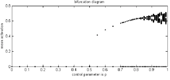
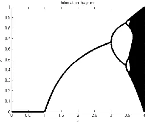
The parameter p (the environmental parameter) is the main source of changing the dynamics (and creating bifurcations) in the conventional logistic map (equation (1)) which can make period-1, period-2 … and chaotic attractors (see the bifurcation diagram of Figure 2). Therefore, it is clear that if we want to model the “interactive” effects of “the environment” on each agent of the network, we have to change the value of in an appropriate manner (due to the activities of the other affecting agents on it).
Figure 2: The bifurcation diagram of the conventional logistic map, ( ) ( ) ( ( )), due the bifurcation parameter, p.
9
2.2.Inter-layer and intra-layer connections
The relationships between layers are determined by the connection matrix CIJ (Appendix A). In this way, if two layers are connected to each other, the value of CIJ is considered to be 1 and if they are not anatomically connected the corresponding CIJ element will be considered to be 0. But the connected areas may affect each other in different ways. So we have to attribute a weight or a strength parameter to those connections, in the form of a weight matrix WIJ. These weights are considered to be random values between 0 and 1. Since we have not inserted any learning algorithm in this model yet, these weights are considered to be fixed during the CA evolution.
We also tried to make the model closer to the reality by considering both excitatory and inhibitory connections between the agents. It is well-known that the balance between excitatory and inhibitory neurons in the cortex is almost 70- 30% [22], or 80-20% [23] [24]. Therefore, among all connections 80% were considered to be excitatory and 20% inhibitory.
It also should be emphasized that although the number of inhibitory connections is less than the excitatory ones, the inhibitory synapses play a very important role in the behavior of the brain. That’s why we considered the amplitudes of the inhibitory weights to be larger than the excitatory ones (in the order of 7-8 times larger) to take their importance into account. This has been also reported in other related works [1].
2.3.Interaction rules
As it was discussed earlier, the most important part of CA based modeling, is the determination of the interaction rules among the agents. We mentioned at the end of
10
section 2.1 that if we want to simulate the effect of the environment on each agent, we would better change the value of of element in layer .
Based on the bifurcation diagram of Figure 2, in the conventional logistic map if
(for example ), chaos is observed (which can be interpreted as a model of chaotic bursts seen in the active state of the neural populations), and if , a stable period-1 behavior is achieved which can be related to the resting state (quiescent) of the netlet. This was used by Lopez et. al. to construct their interesting interaction rule among the logistic-type agents in the modeling of bi-stability in the brain [4]. Lopez used two linear relationships in order to simulate the excitatory and inhibitory forms of interaction as below:
Lopez Interaction Rules [4]:
For agent i of the N elements in a network, we have ̅ ( ), in which the
value ̅ is the effect of other neighboring elements on . This net-effect could be excitatory or inhibitory. This function is selected to be a linear function depending on the actual “local mean value”, of the neighboring signal activity and expanding the interval (0, 4) in the form below:
{̅ ( ) ̅ ( )
(4)
In which: ( ∑ ).
This way, the values of ̅ will always be either 1 or 4, based on the mean activities of the neighbors and their interaction type (i.e. excitation or inhibition). Therefore the interaction of neighbors could make the target agent to become silent (when ̅ ) or to become active in a bursting pattern (when ̅ 4).
11
Most of the researchers like Lopez have used those rules in a “fully excitatory or fully inhibitory” network, with random or regular connections. But here we have considered our model to have 80% excitatory and 20% inhibitory netlets (based on physiological data) and by using the anatomical connections (which was proved to have small world properties [18] [25], which is more realistic connectivity pattern compared to an ordered or a random network). We also used a weighted matrix as inter-layer and intra-layer strength among netlets and considered some synaptic delays as an important property of brain in the realization of our model (see section 2.4). But the most important and novel difference of our proposed model compared to other similar models of neural dynamics, is the way we define “interaction rules” among the agents. Now we are now ready to explain the interaction rules we used for the evolution of our CA:
Proposed Interaction Rules:
We use a modified version of the idea of coupled logistic maps, in a completely different framework which we think is a more realistic one: a multiplicative relationship and a “geometric mean”, instead of the popular “arithmetic mean”, as the total effect of the neighbors.
For an element in a network of coupled logistic-type agents, we have:
̅ ( )
The net effect of excitatory-inhibitory connections from the neighbors is reflected in the value of ̅ in the form of:
̅ ( √∏
∏ ( )
12
This is a “geometric mean” among the neighbors, not the conventional arithmetic mean! We will discuss later that the geometric mean could be a more realistic form of interaction in our model. We borrow a modified version of the definition of excitation and inhibition from the work of Lopez like this:
{ ( ( ) ) ( ( ) )
Therefore, instead of using,
( ) ( ),
We used two different “adaptive” threshold values of and . This could be generally more realistic, because there is no reason that all synapses have the same selection value (or ) to start activation.
The output values of (and ) could be 4 or 1 (1 or 4) based on the values of
and , and also the predefined type of the connection (excitatory or inhibitory).
We believe that the geometric mean is a more realistic interaction rule, than the arithmetic mean in our application. Here we are going to discuss this issue. Consider we want to affect a logistic-type agent (change its dynamical behavior) by changing its gain parameter . Consider that this element has inhibitory and excitatory neighbors. If we use an arithmetic model of interaction, we simply have to use the sum of all excitatory-inhibitory effects as below:
13
∑
∑
(5)
And use it in a suitable coded form in the logistic equation, like equation (4). But this form of mean value, fades or degrades the independent effect of each individual neighbor on the target . However, when a multiplicative interaction in the form of a geometric mean is used, each neighbor affects the target directly and its effect could be studied independently of others without being faded or degraded by them:
√∏
∏
( )
Another potential advantage of this form of coupling is its capability in creating complex behaviors of the neural populations (compared to the simpler linear weighted sum of equation (5)) because of its nonlinearity.
2.4.Time delays
Timings of the activation and inactivation of neurons play a very important role in the overall dynamics of the whole system [26]. This is mainly because of the synaptic delays. On one hand, most of the computational neuroscientists discard delays as some unimportant thing that only complicates modeling. From a mathematical point of view, a system with delays is not finite -but infinite- dimensional, which poses some mathematical and simulation difficulties [26]. On the other hand, others argue that an infinite dimensionality of spiking networks with axonal delays is not a disadvantage but an immense advantage that results in an unprecedented information capacity. Izhikevich even claims that there are some stable firing patterns that are not possible without the
14
delays [26]. We are not also going to neglect the intrinsic role of delays of the neural system in our modeling.
In the original form of netlets’ activation function (equation (2)), which we used logistic equation as its model, the time has been quantized in units of the synaptic delay , and it is assumed that the neurons can fire only at times which are integral multiples of [20]. Therefore, each discrete time step in the logistic map refers to the continuous time interval of . Hence, the discrete value of corresponds to in the continuous time scale. But what is the value of itself ?
Some researchers argue that the synaptic delays and the refractory periods generally are found to be close to 0.5 ms and 1ms, respectively [20]. Another report about this quantity is of the order of 1-3 ms [1]. But the report of Izhikevich from the synaptic delays seems more realistic, since it covers a broader interval and talks mainly about the neocortex: “A careful measurement of axonal conduction delays in the mammalian neocortex showed that they could be as small as 0.1 ms and as large as 44 ms, depending on the type and location of the neurons [26]”.
In our work, we considered the specific value of for the mean time interval between two activations. This value is important and mainly adopted because we are going to use the time delays present “between” processing layers of visual system in our model. The latencies between the processing layers of the ventral pathway in the visual system have been reported in [27] [28] and could be seen schematically in Figure 3. We used this platform in order to estimate the other latencies between the layers of our model.
15
Figure 3: adopted from [28]: the latencies between the layered structure of the ventral pathway (from retina to STPa), in miliseconds.
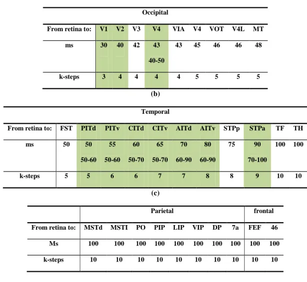
It should be emphasized here that although our model is a behavioral and functional model, we are trying to use as much structural and physiological data as possible, because in any complex system, the structure could not be separated from the function. Based upon the above discussion and by using the data in Figure 3 and the connection matrix of macaque visual cortex, we estimated the other between-layer latencies in the form of discrete time steps of our logistic-type model (see Table 1).
By using the above updating rules for each element of our cellular automata, we are now ready to simulate the proposed model and validate some of our statements about the applicability of such a model in mimicking the visual perceptual dynamics.
16
Table 1: Travel time from retina to different visual processing layers of our model (first row: in mili-seconds, second row: in the discrete time interval, normalized to the time unit ). The shaded columns contain the exact values from Figure 3, other columns were estimated based on the shaded ones. for (a) Occipital cortex, (b) Temporal cortex, (c) Parietal and frontal cortex.
(a)
Occipital
From retina to: V1 V2 V3 V4 VIA V4 VOT V4L MT
ms 30 40 42 43
40-50
43 45 46 46 48
k-steps 3 4 4 4 4 5 5 5 5
(b)
Temporal
From retina to: FST PITd PITv CITd CITv AITd AITv STPp STPa TF TH
ms 50 50
50-60 55 50-60 60 50-70 65 50-70 70 60-90 80 60-90
75 90
70-100
100 100
k-steps 5 5 6 6 7 7 8 8 9 10 10
(c)
Parietal frontal
From retina to: MSTd MSTI PO PIP LIP VIP DP 7a FEF 46
Ms 100 100 100 100 100 100 100 100 100 100
k-steps 10 10 10 10 10 10 10 10 10 10
3. Simulation results
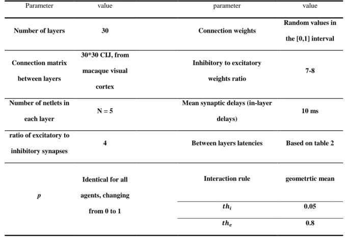
The summary of our selected values of parameters and the global framework of modeling are shown in Table 2. Under these situations, the whole model is capable of showing different kinds of dynamical behaviors and attractors depending on different perceptual situations.
17
Table 2: simulation framework and selected values of parameters.
Parameter value parameter value
Number of layers 30 Connection weights
Random values in the [0,1] interval
Connection matrix between layers
30*30 CIJ, from macaque visual
cortex
Inhibitory to excitatory weights ratio
7-8
Number of netlets in each layer
N = 5
Mean synaptic delays (in-layer delays)
10 ms
ratio of excitatory to inhibitory synapses
4 Between layers latencies Based on table 2
p
Identical for all agents, changing
from 0 to 1
Interaction rule geometrtic mean
0.05
0.8
In our first experiments, we suppose that all agents in all layers have the same value of parameter (see equation (3)), i.e. [ ] [ ]. Then we studied
different behaviors of the CA using the bifurcation diagram due to parameter . After that different values of were studied in the model. The output value selected for this model is considered to be “the mean activation of the whole network in each iteration”, as an estimation of cortical electrical activities recorded by the EEG or ECoG electrodes [11]. We also study the synchronization and desynchronization properties of the netlets using correlation values in different environmental situations [29] [11]. The detailed results are presented in the following sub-sections.
18
3.1.Different dynamics, bifurcation diagram
The bifurcation diagram of the CA under the conditions described in the previous sub-section is presented in Figure 4. Here all of the agents are considered to have the same value of . The network starts from the same initial condition each time, and evolves to its attractor after 500 iterations. Updating of the CA is performed synchronously. It can be seen from the bifurcation diagram that the system is capable of showing different dynamical states which could be interpreted as one of the widespread perceptual states of the visual system.
In Figure 5-a, the CA shows a period-1 behavior around 7. This period-1, or fixed point behavior could be representative of a state that the visual system settles into a fixed attractor, i.e. recognizes a stimulus. Figure 5-b on the other hand, shows a period-2 situation for 83 which can be a model of bi-stable perception. The bi-stability and the multi-stability in general, is an interesting phenomenon studied in the literature with great interest in recent years [30] [31] [4].
Figure 4: bifurcation diagram of the CA, as a function of control parameter for threshold values of .
19
For example, a bi-stable perception could be happened in visual system while observing the simple shape of Figure 6. In this shape the perceptual dynamics switches between the image of “two faces” and the image of “a vase” in the middle part. Any of these perceptions can be modeled as one of the stable states in the period-2 region of the CA. the perceptual system of the brain switches between these two stable points in a periodic way which represents the period-2 solution. The more complex situation of period-8 which is indicative of an 8-stable situation, occur for 6 (Figure 5-c).
But the most interesting behaviors could be seen in Figure 5-d to Figure 5-f as the non-periodic cases. It could be seen in Figure 5-d that for , a two-part non-periodic attractor appears which could be interpreted as a “blur” bi-stable perception of a stimulus, or a 2-tori quasi periodic response. When our visual system has not reached to a single decision about a stimulus and is searching around two possible answers!
Figure 5-e and Figure 5-f show a chaotic attractor. We can interpret this attractor as the baseline behavior of the brain, when it has not been encountered to a new stimulus. This baseline is the main dynamical state of the brain, from which it could be attenuated due to an external stimuli (scene, odor, …). Hence in the presence of an external stimulus, this attractor changes into one (or some) ordered attractor(s), called liquid-like quasi-attractors, corresponding to that specific stimulus [11] [10]. Then it again comes back to this baseline chaotic attractor, in order to be ready to interact with the next and next changes in the environment. The real chaotic dynamic of the brain, could be interpreted as the searching state of the brain in its basin of attraction, coming into and going beyond the chaotic and non-chaotic attractors.
20
(a) (b)
(c) (d)
(e) (f)
Figure 5: different dynamical behaviors of the CA, top plot: the time series, bottom plot: the phase portrait, (a) period-1, for 7, (b) period-2, for 83, (c) period-8, for , (d) two-part non-periodic attractor, for , (e)-(f) chaotic attractors, for 3 and respectively.
21
It could be seen from Figure 7 that the frequency content of this chaotic signal is comparable with the spectrum that is seen in the normal EEG signal [8].
Figure 6: a bi-stable perceptual situation could occur by the visual system in the observation of this simple shape: a vase or two faces? This bi-stability could be modeled by the period-2 behavior of the CA model.
a b
Figure 7: (a) EEG spectra for different EEG electrodes. (b) The spectra of the chaotic output signal of the CA, for for . It could be considered to have a form, comparable with the normal EEG.
22
3.2.A more realistic situation
In the previous part, like many other related works [21] [4], we assumed that all of the agents have the same bifurcation parameter (i.e. in equation (3)). Indeed, this could
not be the real situation; there is no reason for all neural populations to have the same value of in general. Rather, the dynamical state and properties of each neural population may be different from the others. Hence, a more realistic approach of modeling is to consider each agent to have its own value of which is not necessarily equal to the other agents.
In order to do that, we considered some random values for parameter of each agent. The result showed a more similar behavior to real EEG signals in the form of its spectra and the synchronization- desynchronization patterns of 150 agents which can resemble the functional relationships and synchrony among different neural populations of the visual system (Figure 8).
The synchronization pattern is calculated between each agent and the mean activation of the network (the ensemble), in a window size of 50 samples, for a total size of 500 iterations (by the “xcorr” matlab function) [29].
23
(a) (b)
(c)
Figure 8: (a) The time evolution and phase portrait of the chaotic output signal of the CA with different values of parameter each agent (values selected randomly between 0-1). (b) The spectra
of part (a), (c) The synchronization-desynchronization pattern of all agents during the evolution of the CA in 500 steps, in terms of correlation coefficient measure.
24
4. Discussion
A model of visual perceptual dynamics based on cellular automata and the anatomical connection matrix was introduced. The model is a behavioral and phenomenological model which tries to take into account as much physiological and anatomical considerations as possible; such as anatomical connection matrix of macaque visual cortex, netlet dynamics, excitatory-inhibitory synapses with appropriate ratio and weight, in-layer delays and between layer latencies. This model is one of the most complete models proposed for neural dynamics, which considers anatomical connections in combination with a CA approach using chaotic maps.
One of the most important advantages of using CA for our modeling was that Cellular automaton is a modeling tool capable of modeling large scale complex systems, which gives the ability to study the system from microscopic to mesoscopic and macroscopic levels. It also makes it possible to define and tune the appropriate interaction rules in order to reach to the desired behavior from the whole system.
We introduced a new interaction rule based upon the “geometric mean” value (a nonlinear synaptic function) and multiplicative relationship among the agents. We claim that it is more realistic than the previous arithmetic mean and linear interaction rules, because it gives the possibility of changing and studying each neighbor individually, without being degraded by the others. We also used adaptive thresholds in our synaptic decision makings.
It was shown that the proposed model is capable of showing different dynamical behaviors seen in visual perceptual framework, from a fixed stable attractor to bi-stable, multi-stable and chaotic behaviors. The chaotic signal was shown to have a form of
25
frequency spectrum comparable with the spectrum of a normal EEG. We also showed that the synchronization-desynchronization pattern of the agents in their evolution is close to reality in the chaotic mode.
The future works on this model should consider the effects of learning and seeing different scenes on the model parameters, based on a suitable learning approach such as STDP. It may also be developed by considering two-dimensional CAs instead of current one-dimensional form, for each layer. Besides, some visual perceptual deficits such as face recognition problems seen in the Autism disorder may be behaviorally modeled by this model in the future.
5. References
[1] M. Barbosa, K. Dockendorf, M. Escalona, B. Ibarz, A. Miliots, I. Nadal-Sendina, G. Zamora-Lopez, L. Zemanava. "parallel computation of large Neuronal Networks with structured connectivity." Lectures in Supercomputational Neuroscience: Dynamics in Complex Brain Network, Springer, pp. 343-367, (2008).
[2] N. H. Packard, S. Wolfram. "Two-Dimensional Cellular Automata." J. Stat. Phys.
38(5/6). pp. 901-946, (1985).
[3] "Cellular automaton," Wikipedia, the free encyclopedia, 3 September 2014.
[Online]. Available: http://en.wikipedia.org/wiki/Cellular_automaton. [Accessed 27 10 2014].
[4] R. Lopez-Ruiz, D. Fournier-Prunaret. "The bistable brain: a neuronal model with symbiotic interactions", Book Chapter: Symbiosis, Evolution, Biology and Ecological Effects, pp. 235-253, (2013).
[5] R. Kozma, M. Pulji. "Hierarchical random cellular neural networks for system-level brain-like signal processing." Neural Networks45, pp. 101-110, (2013).
[6] F. R. Adams, H. T. Nguyen, R. Raghavan, J. Slawny. "A parallel network for visual cognition." IEEE Trans. Neural Netw3(6), pp. 906-922, (1992).
[7] T. A. Mattei, "The fuzzy logic of degenerative disc disease: from a lorenz attractor to a percolation threshold model," World Neurosurg 80 , pp. 8-12 (2013).
[8] R. Kozma, M. Puljic. "Chaotic Behavior in Probabilistic Cellular Neural Networks." The International Joint Conference on Neural Networks (IJCNN). Barcelona: IEEE, pp. 1-7, (2010).
26
[9] M. Beigzadeh, S. M. R. Hashemi Golpayegani, Shahriar Gharibzadeh. "Can cellular automata be a representative model for visual perception dynamics?" Front. comp. Neurosci.7(130) (2013).
[10] W. J. Freeman, "The Physiology of Perception," SCI AM, 264, pp. 78-85, (1991). [11] R. Kozma, M. Pulji, W. J. Freeman. "THERMODYNAMIC MODEL OF
CRITICALITY IN THE CORTEX BASED ON EEG/ECOG DATA," Book Chapter in Criticality in Neural Systems, Berkeley, John Wiley & Sons, Inc. (2012)
[12] S.C. Ponten, A. Daffertshofer, A. Hillebrand, C.J. Stam. "The relationship between structural and functional connectivity: Graph theoretical analysis of an EEG neural mass model." NeuroImage52, pp. 985–994, (2010).
[13] O. Sporns, "Small-world connectivity, motif composition and complexity of fractal neuronal connections," BioSystems, 85, p. 55–64, (2006).
[14] C. J. Stam, J. C. Reijneveld. "Graph theoretical analysis of complex networks in the brain." Nonlinear Biomed Phys1(3), pp. 1-19, (2007).
[15] O. Sporns, "Contributions and challenges for network models in cognitive neuroscience," Nat. Rev. Neurosci, 17, pp. 652-660, (2014).
[16] D. J. Felleman, D. C. Van Essen. "Distributed Hierarchical Processing in the Primate Cerebral Cortex." Cereb. cortex1, pp. 1-47, (1991).
[17] O. Sporns, "Connectivity network data sets," 2000. [Online]. [Accessed 2013]. [18] O. Sporns, J. D. Zwi. "The Small World of the Cerebral Cortex." Neuroinform2 pp.
145-162, (2004).
[19] P.A. Anninos, B Beek, T.J. Csermely, E.M. Harth, G. Pertile. "Dynamics of Neural Structures." J. Theor. Biol.26, pp. 121-148, (1970).
[20] E.M. Harth, T.J. Csermely, B Beek, R.D. Lindsay. "Brain Functions and Neural Dynamics." J. Theor. Biol.26 pp. 93-120, (1970).
[21] R. Pashaie, N. H. Farhat. "Self-Organization in a Parametrically Coupled Logistic Map Network: A Model for Information Processing in the Visual Cortex." IEEE Trans. Neural Netw20(4), pp. 597-608, (2009).
[22] X. Chen, R. Dzakpasu, "Observed network dynamics from altering the balance between excitatory and inhibitory neurons in cultured networks," Phys. Rev. E. 82
(2010).
[23] P. D. King, J. Zylberberg, M. R. DeWeese, "Inhibitory interneurons enable sparse code formation in a spiking circuit model of V1," BMC Neuroscience. 13.1, pp. 148-149, (2012).
[24] A. Metaxas, R. Maex, V. Steuber, R. Adams, N. Davey, "The effect of different types of synaptic plasticity on the performance of associative memory networks with excitatory and inhibitory sub-populations," in Lecture Notes in Computer Science (including subseries Lecture Notes in Artificial Intelligence and Lecture Notes in Bioinformatics), pp.136-142, (2012).
[25] M. Rubinov, O. Sporns, "Complex network measures of brain connectivity: Uses and interpretations," NeuroImage. 52, pp. 1059–1069, (2010).
[26] E. M. Izhikevich, "Polychronization: Computation with Spikes," Neural Comput,18, pp. 245–282, (2006).
27
[27] M. W. Oram, D. I. Perrett. "Modeling Visual Recognition From Neurobiological Constraints." Neural Networks 7(6/7), pp. 945-972, (1994).
[28] L. Wiskott, "How Does Our Visual System Achieve Shift and Size Invariance," Problems in Systems Neuroscience, (2004).
[29] M. Puljic, R. Kozma, "Synchrony in Probabilistic Cellular Automata," University of Memphis, Memphis, (2005).
[30] N. Nagao, H. Nishimura, N. Matsui. "A Neural Chaos Model of Multistable Perception." Neural. Process Lett12(3), (2000).
[31] Y. H. Zhou, J. B. Gao, K. D. White, I. Merk, K. Yao. "Perceptual dominance time distributions in multistable visual perception." Biol Cybern90(4), pp. 256-263, (2004).
28
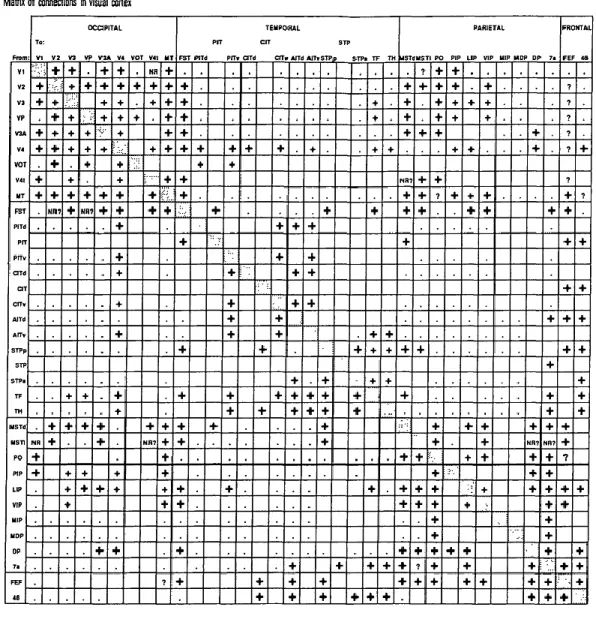
Appendix A: The 35*35 connectivity matrix of Felleman and Essen [16]
Table 2: this table is a connectivity matrix for interconnections between areas in the macaque visual cortex. Each row shows whether the area listed on the left sends outputs to the areas listed along the top. Conversely, each column shows whether the area listed on the top receives input from the areas listed along the left. Large plus symbols (+) indicate a pathway that has been reported in 1 or more full-length manuscripts. Small plus symbols indicate pathways only in abstracts or unpublished studies. Dote (.) indicate pathways explicitly tested and found to be absent. Blanks indicate pathways not carefully tested for. Question marks (?) denote pathways whose existence is uncertain owing to conflicting reports in the literature. “NR” and “NR?” indicate nonreciprocal pathways, i.e. connections absent in the indicated direction even though the reciprocal connection has been reported. Shaded boxes along the diagonal represent intrinsic circuitry that exists whitin each area: these are nor indicated among pathways tabulated in the following table. Adopted from [16].
![Figure 3: adopted from [28]: the latencies between the layered structure of the ventral pathway (from retina to STPa), in miliseconds.](https://thumb-us.123doks.com/thumbv2/123dok_us/8381702.2226827/15.918.204.717.110.561/figure-adopted-latencies-layered-structure-ventral-pathway-miliseconds.webp)