RESEARCH ARTICLE
10.1002/2015JC011111
Complex coastal oceanographic fields can be described by
universal multifractals
Jozef Skakala1and Timothy J. Smyth1
1Plymouth Marine Laboratory, Plymouth, UK
Abstract
Characterization of chlorophyll and sea surface temperature (SST) structural heterogeneity using their scaling properties can provide a useful tool to estimate the relative importance of key physical and biological drivers. Seasonal, annual, and also instantaneous spatial distributions of chlorophyll and SST, determined from satellite measurements, in seven different coastal and shelf-sea regions around the UK have been studied. It is shown that multifractals provide a very good approximation to the scaling proper-ties of the data: in fact, the multifractal scaling function is well approximated by universal multifractal theory. The consequence is that all of the statistical information about data structure can be reduced to being described by two parameters. It is further shown that also bathymetry scales in the studied regions as multifractal. The SST and chlorophyll multifractal structures are then explained as an effect of bathymetry and turbulence.1. Introduction
A fractal [Mandelbrot, 1982] is a scale-invariant set of points typically characterized by a parameter known as the fractal dimension. A multifractal is a scale-invariant field characterized by a spectrum of fractal dimen-sions (see reviews inTel[1988],Schertzer et al. [2002], andSchertzer and Lovejoy[2011]). In the theory of tur-bulence [Richardson, 1922;Kolmogorov, 1941], the conserved energy flux shows significant intermittency [Novikov and Stewart, 1964;Yaglom, 1966;Mandelbrot, 1974] leading to corrections to the Obukhov scaling law [Obukhov, 1949]. Multifractality reflects statistical scale invariance of the energy flux distribution [ Schert-zer and Lovejoy, 1987]. Multifractal theory has now been applied to a diverse range of disciplines such as geology, finance, and climate research [Mandelbrot, 1997;Harte, 2001;Lovejoy and Schertzer, 2013;Lovejoy, 2014].
There are very few mechanisms in nature that could constrain scale invariance to a discrete sequence of scales. A phenomenon is often expected to be scale invariant at each scale within a certain range of scales (that is scale invariant on a continuous number of scales). Continuous scale invariance puts significant math-ematical constrains on the multifractal model, and only specific classes of continuous cascade models exist [Seuront et al., 2005]. The most successful continuous multifractal model is universal multifractals (UM) [Schertzer and Lovejoy, 1987, 1988, 1997, 2011].
In oceanography, universal multifractals have already found application using the Fractionally Integrated Flux (FIF) model [Schertzer and Lovejoy, 1987, 1988] to time series obtained from in situ measurements of various oceanographic tracers [Seuront et al., 1996a, 1996b;Seuront and Lagadeuc, 1997;Seuront et al., 1999;
Seuront and Schmitt, 2005a,b] and more recently to satellite chlorophyll data [de Montera et al., 2011]. The main purpose of these studies is to analyze the level to which turbulence influences the oceanographic field structure formation. Sea surface temperature (SST) is generally expected to behave as a passive scalar [ Love-joy et al., 2001a] (tracer passively advected by a parcel of fluid). In the case of chlorophyll, the situation is much more puzzling [Martin, 2003;de Montera et al., 2011]. In general, biological activity (zooplankton graz-ing) is expected to significantly modify the phytoplankton scaling relation. This is, however, expected to happen predominantly at planktonscale (30–500 m) [Currie and Roff, 2006]. What happens on larger scales than planktonscale is a matter of debate. Some results suggest a mixed turbulence-growth regime [Lovejoy et al., 2001a,b]. An increasing number of results [de Montera et al., 2011;Nieves et al., 2007;Currie and Roff, 2006;Seuront et al., 1999], however, indicates that chlorophyll on the scales larger than planktonscale exhib-its scaling properties at least similar to the scaling of a passive tracer.
Key Point:
The time median chlorophyll and SST spatially scale as universal multifractals
Correspondence to: J. Skakala, [email protected]
Citation:
Skakala, J., and T. J. Smyth (2015), Complex coastal oceanographic fields can be described by universal multifractals,J. Geophys. Res. Oceans, 120, 6253–6265, doi:10.1002/ 2015JC011111.
Received 6 JUL 2015 Accepted 31 AUG 2015 Accepted article online 3 SEP 2015 Published online 15 SEP 2015
VC2015. American Geophysical Union. All Rights Reserved.
Journal of Geophysical Research: Oceans
PUBLICATIONS
Patchiness of an oceanographic field is a result of many drivers acting to increase or decrease heterogeneity at different scales [Martin, 2003;Mahadevan, 2004]. Previous work largely focused on analysis of time series data/satel-lite overpass imagery, but field heterogeneity can be analyzed from many other perspectives. This paper sets out to partially address that gap by looking at regional geographic distributions (see Figure 1) of SST and chlorophyll-a in the shelf seas. These geographic distributions are characterized by suitable time median (annual/seasonal median) data. Many drivers cre-ate structures that domincre-ate field spatial heterogeneity in the time series data, but spatially average out in annual/seasonal median data. Only some of the structures corresponding to some specific drivers survive in time medians. In the shelf seas, one expects bathymetry to be the main driver of SST and chlorophyll geography. Bathymetry influences SST directly, but mainly affects both chlorophyll and SST via influencing the currents. It has a dominant influence on tidal cur-rents and bathymetry might potentially create inhomogeneities in turbulence that do not average out in the time median data. Bathymetry also determines the dominant regions of upwelling, which significantly influen-ces both SST and chlorophyll (however, we do not expect that wind-driven upwelling is important in the regions explored in this paper).
Our working hypotheses can be summarized as follows: (a) bathymetry is multifractal (this is often the case for earth topography [Lavalee et al., 1993;Gagnon et al., 2006]), (b) SST and chlorophyll scale at least simi-larly to a passive tracer, (c) geography of annual/seasonal median chlorophyll and SST data will be a result of a combined effect of bathymetry and (inhomogeneous) turbulence, and (d) the combined effect of those two multifractal structures (bathymetry and turbulence) will be a multifractal structure. The last point means we predict that the spatial scaling of SST and chlorophyll geography will be well described by a multifractal model. Some further consequences of this hypothesis and more exact predictions will be presented in the next section of the paper.
The important novel contribution of this paper is finding a multifractal interplay between oceanographic field geography and drivers. As well as this, the paper carries out a scaling analysis of space-time variability in chlorophyll and SST. The range of scales at which space-time SST and chlorophyll have been analyzed in this paper compares well with two previous papers [de Montera et al., 2011;Nieves et al., 2007]. Both papers dealt with very specific regions, and this paper provides more evidence to better understand chlorophyll and SST scaling at the submesoscale and mesoscale.
2. Method
2.1. Theory
In this work, the stochastic (rather than geometric) approach to multifractals [Schertzer and Lovejoy, 1987, 1988, 2011;Lovejoy et al., 2001b] is used. Multifractal formalism is best introduced within the context of
Figure 1.The image shows annual median SST distributions (SST geographical character-istics) in 2009. It marks the regions in which the median data are analyzed: (a) Irish Sea, (b) Bristol Channel, (c) Celtic Sea I, (d) coastline of Devon, (e) English Channel, (f) Celtic Sea II, and (g) Brittany coastal region.
passive oceanic tracers and turbulence, as this is its dominant application in oceanography [Schertzer and Lovejoy, 1987;Seuront et al., 1996a, 1996b;Seuront and Lagadeuc, 1997;Seuront et al., 1999;Seuront and Schmitt, 2005a, 2005b;de Montera et al., 2011].
The increments of turbulent longitudinal velocity field (v) and passive scalar field (q) were predicted by Kol-mogorov[1941] andObukhov[1949] to scale as:
Dv‘ hjvðx1‘Þ2vðxÞji ’ h‘i1=3‘1=3; (1) Dq‘ hjqðx1‘Þ2qðxÞji ’ h/‘i
1=3
‘1=3; (2)
/5v1=221=6; (3)
where;vare fluxes conserved by the dynamical equations and‘is the scale of separation between points. The theory of Kolmogorov [1941] and Obukhov [1949] is based on the assumption that the fluxes are (almost) homogeneous. However, this assumption was criticized a long time ago byLandau and Lifshitz
[1963]. Nowadays, it is widely accepted that the fluxes are significantly intermittent at different scales, and this leads to corrections to the scaling exponents from equations (1) and (2). One can incorporate intermit-tency into the passive tracer (q) model as follows [de Montera et al., 2011]:
Dqq‘ hjqðx1‘Þ2qðxÞjqi ’ h/aq‘ i ‘qH: (4) Conserved flux/in equation (4) scales as a multifractal cascade and the equation describes scaling of dif-ferent powersq. The intermittency of the field depends on the specific multifractal cascade model of/. Apart from specifying multifractal cascade/, the model from equation (4) has two more free parameters,
aandH.
Multifractal cascade/can be best described through the scaling of its statistical moments:
h/q‘i ’‘2KðqÞ; (5)
whereK(q) is referred to as the scaling moment function. The other important multifractal characteristics like singularity fractal dimensions or statistical exponents (fractal codimensions) can be derived fromK(q) with the help of Legendre transform [Schertzer and Lovejoy, 1987, 2011]. Since turbulence occurs at every scale, one expects the scaling described by the equation (5) to be valid for continuous number of scales. The limit of continuous scaling significantly constrains the class ofK(q) functions [Seuront et al., 2005]. The universal multifractal model is a specific case that defines the continuum scaling limit for stable cascades. The scaling moment functionK(q) is obtained in a specific, simple universal form [Schertzer and Lovejoy, 1987, 1988, 2011;Schmitt et al.,1993]:
KðqÞ5 C1
a21ðq
a2qÞ;0a2;a6¼1; (6)
and
KðqÞ5C1qlnðqÞ;a51; (7)
whereaandC1are two free, but constrained, parameters of the model.C1parameter is a fractal
codimen-sion of the set that gives dominant contribution to the mean, andadescribes how rapidly fractal dimen-sions of sets vary as they leave the mean singularity [Gagnon et al., 2006]. Special case of a52 is the lognormal model of turbulence [Gurvitch and Yaglom, 1967].
Assuming that flux/scales as universal multifractal, one can suitably redefineC1;Hparameters and replace
the model given by equation (4) by a simpler model with only three parametersC1;a;H[Lavalee et al., 1993;
de Montera et al., 2011]:
Dqq‘ ’ h/q‘i ‘qH: (8)
Hereq scales again as universal multifractal with some new C1;aparameters (equation (6)). The model
given by equation (8) is called Fractionally Integrated Flux (FIF) model [de Montera et al., 2011] and the model was first used bySchertzer and Lovejoy[1987] to model rain and clouds. TheHparameter in the equa-tion (8) gives the increments scaling for the powerq51. In the original model of Kolmogorov 3-D isotropic
turbulence (equation (2)),H51/3; however, in the intermittent case described by the FIF model, H can divert from the Kolmogorov value. The exact value of turbulentHdepends on the details of the model, and to estimate it, one has to make additional assumptions. Despite this, it is generally expected thatHdoes not divert radically for 3-D turbulence from the nonintermittentH51/3 and can be assumed to be some-where around 0.3–0.4. However, in the ocean for scales>1 km, the horizontal dimensions become large when compared to the vertical dimension, with very different physics in vertical and in horizontal, and in such a situation, the relevance of the Kolmogorov isotropic 3-D theory is questionable. It is sometimes assumed (based on anisotropic models [Lovejoy and Schertzer, 2010]) thatH51/3 will remain in horizontal dimensions on large scales. Other authors [i.e.,Currie and Roff, 2006] suggest that H can lie anywhere between 0:33 and 1, withH51 being the idealized 2-D turbulence value. Fields that are assumed to be pas-sive tracers, like SST, are then used (in the 2-D-like cases [seeCurrie and Roff, 2006]) to find a reference value forH. Since the present paper deals with shallow shelf sea regions (average depth between 35 and 100 m), and horizontal scales much larger than 1 km scale, one has to be aware of potential (other than intermit-tency) corrections to the Kolmogorov value of the scaling exponent.
Scaling of field increments has implications for multifractality of field itself: various mathematical results [Cates and Deutsch, 1987;Siebesma and Pietronero, 1988] suggest that field spatial correlations described by power laws (such as the equation (8)) imply that the field is a multifractal distribution. Suppose now that also different powersqof bathymetry increments scale as a power law, bathymetry increments (q51) then scale with someHexponent. If the hypotheses from section 1 are valid, we expect that SST and chlorophyll increments will also follow a power law with theirHexponents somewhere between theHof bathymetry and theHof turbulence. It is to be then expected [Cates and Deutsch, 1987;Siebesma and Pietronero, 1988] that SST and chlorophyll are themselves multifractal.
2.2. Data and Analysis
Sea surface temperature (SST) data were obtained from the NOAA Advanced Very High Resolution Radia-meter (AVHRR) satellite series and processed at the Plymouth Marine Laboratory by the NERC Earth Obser-vation Data Acquisition and Analysis Service (NEODAAS) for the period 1998–2012. Ocean color data from the Sea-viewing Wide-Field-of-view Sensor (SeaWiFS) were also processed by NEODAAS for more con-strained period 1998–2004 to obtain chlorophyll [O’Reilly et al., 1998].
The advantage of using satellite data fields is the wide spatial coverage and subsequent large data volumes that are available. Both the SST and chlorophyll data have a nominal resolution of 1.1 km and reveal a large amount of heterogeneous structure when single overpass images are obtained. However, the disadvantage of using satellite remote sensing techniques to determine SST and chlorophyll can be the data coverage issue: especially in midlatitude and high-latitude areas, clear sky imagery is relatively rare because of cloud cover. To use multifractal techniques, near-total area coverage is required when scaling from 1 to
100 km for specified regions. Using multifractal techniques is therefore limited for single overpass imagery to exceptionally clear scenes. The problem is much less present in the field geography data: the annual and seasonal time median data are by definition less data sparse and noisy than single overpass imagery. First the idea that annual/seasonal median spatial distributions scale as multifractals will be explored. If the multifractal scaling is observed, one tries to fit the data by a specific multifractal model, such as universal multifractals. One then explores the validity of the hypothesis presented in section 1 to explain the observed multifractal scaling. This means that one analyses theqth power of bathymetry (B) increments scaling (DBq‘ defined in the equation (8)) and determines if the scaling follows a power law. One further analyses SST and chlorophyll increments scaling. By comparing the values ofH(field increments scaling exponent from the equation (8)) for different fields, the validity of the hypothesis presented in section 1 of this paper can be explored.
The scaling analysis was carried out for seven shelf-sea regions around the south-west of the UK marked in Figure 1 over multiple year annual chlorophyll and SST data. The regions chosen were: (i) two regions in the Celtic Sea (called ‘‘Celtic Sea I’’ and ‘‘Celtic Sea II’’), which extended to scales2102250 km; (ii) the Irish Sea region extending up to 150 km; (iii) the English Channel region extending to 215 km; (iv) region in Bristol Channel that extends to 100 km scale; (v) region around Brittany, extending to 130 km scale and finally; (vi) region around the coast of Devon extending to over 100 km scale. The Bristol Channel region was excluded from the chlorophyll data analyses as large concentrations of sediment in this region are known to
invalidate the remote sensing chlorophyll algorithm. Bathymetry data were used to carry out a scaling anal-ysis for the seven regions (Figure 1): these were obtained from the Liverpool Coastal Observatory and are from the POLCOMS high-resolution continental shelf (HRCS) model. The bathymetry data had a (coarser) resolution of 1.8 km.
To get additional insight into the space-time fields, the analysis of the single overpass SST and chlorophyll satellite imagery is provided. For SST, all seven regions were considered and, depending on the region, between 24 and 37 clear scenes were visually selected (the number of selected images depended on the number of sufficiently cloud-free scenes). For chlorophyll, only noncoastal four regions (Celtic Sea, Celtic Sea II, English Channel, and Irish Sea) were considered, and for each region, between 19 and 27 clear scenes were selected.
To calculate the cascade model scaling properties, the standard method of moments was used. This consists of calculatinghqq‘i, which involves averagingqq‘;iover boxes labeled byi, whereqq‘;iis aqth power of a suit-ably normalized localith box field (q) average. The field value was normalized by the regional field average and the scale‘is the square root of the box area.
The degree to which the logarithm ofhqq‘iagainst the logarithm of scale behaves as a straight line is then determined: a straight line implies thathqq‘ifulfils equation (5). If the power scaling law (equation (5)) is resultant, theK(q) function is determined by performing for eachqa linear regression of the log-log curve. The final step is to provide the UM fit (see equation (6)) toK(q).
Particular care needs to be exercised over what range of momentsqis analyzed: large moments are very sensitive to extreme value statistics and need large volumes of data to be estimated. For example, recent lit-erature has contained discussions about whether or not it is reasonable to include momentsq>2 in stand-ard multifractal analysis [Lombardo et al., 2014;Schertzer, 2013]. It is also well known that a breakdown of estimating the moments scaling from finite data can show as a second-order phase transition [Schertzer and Lovejoy, 1992, 2011]. The second-order phase transition means the discontinuity in the second derivative of the moments scaling functionK(q), and the name originates from the well-known analogy between multi-fractals and thermodynamics [e.g.,Tel, 1988]. Preliminary analysis showed that for chlorophyll fields, the second-order phase transition occurred at aroundq55, this is similar to the observations ofSeuront et al. [1996a, 1999] for the moments scaling function of fluxes; for SST, there was no clearly visible transition point even forq25. This work only uses moments 0<q2 in the final UM fit. Some test calculations were done for UM fit using 0<q5 with only relatively small changes to the result obtained with 0<q2. (The change toawas within 5%, the change toC1was in some cases larger, between 20 and 30%.)
The shape of the box, or degree of anisotropy, may also be important. In this work, rectangular boxes with sides parallel to longitudes and latitudes were used. The anisotropy was measured by ratior, defined as the ratio between the box sides parallel to longitude and to latitude. Calculations were performed for 1=8r8. For each region, the region natural anisotropy factorrminwas found, a factor that minimized
the heterogeneity of the data. Such an anisotropy factor is thought to correspond to the direction of domi-nant currents in the region.
Special care was taken regarding how to incorporate the idea of scale transition (i.e., from shorter to longer length scales). The box area was changed in each step by 1%, which is not too far from the idea of a ‘‘contin-uous’’ scale transition. Now, if‘is the scale in pixels,‘2is meant to be the number of pixels included in the box. However, there could always be boxes with less pixels than‘2. The first reason for this is that a box can contain land, and one does not include land pixels in the analysis. A second reason is that from the geomet-rical point of view, dividing bounded region into boxes all with the same size would strongly limit the num-ber of discrete scales. The solution was to include boxes with less pixels than‘2, but they were included with a proportionally lower weight, weight proportional to the number of pixels in the box that contribute to the calculation.
Finally, the field increments can be sensitive to both statistical and systematic noise. To improve the accuracy of the increments scaling analysis, the data were averaged over 333 pixel bins. To ensure that this smoothening does not have a significant effect on the analysis, the incremental scaling was ana-lyzed from scales>8 km. To remove near-cloud and nearshore effects, only bins with 9 pixels were considered.
3. Results
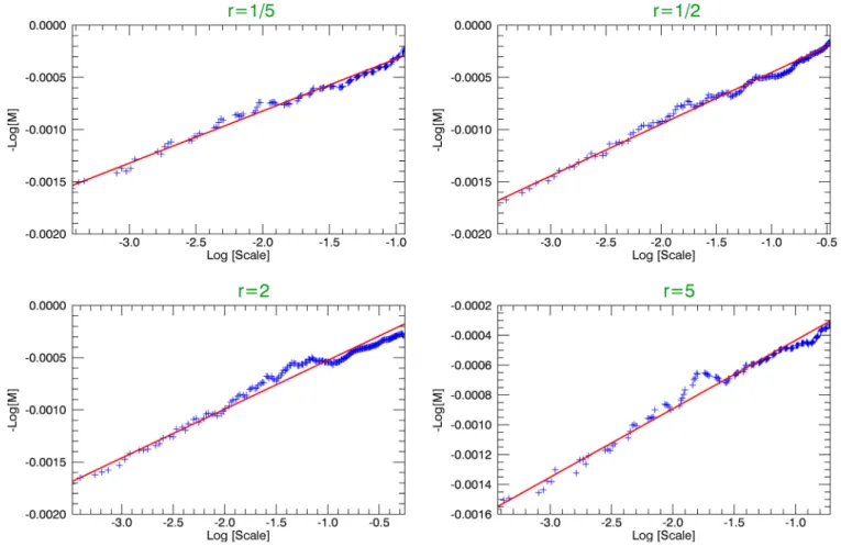
The effect of the shape (degree of anisotropy) of the rectangular box at the scaling property was investi-gated first. Figure 2 shows a typical result (2009 median SST for the Irish Sea): the plots in Figure 2 show scaling of logarithm of the statistical momentq52 (equation (5)) as a function of logarithm of‘=‘regfor
dif-ferent anisotropy coefficientsr.‘=‘regis a ratio between the scale at which the statistical moment was
com-puted and the scale of the region (which is the maximal scale). Straight line in the log-log plot in Figure 2 confirms multifractal scaling (equation (5)). The slope of the linear regression is the value of the moments scaling functionK(2). In Figure 2, one can see that the slope of the linear regression does not change signifi-cantly withr. Indeed, the difference to the value ofK(2) when varyingrfromr51/5 tor55 was less than 8%. In general, for all areas and time periods, it was found that the multifractal properties of the data changed very little withr. Larger deviations are only encountered at extreme values such asr8 or
r1=8.
The SST data show reasonably consistent annual patterns across different years (1998–2012) in all regions explored. For the lack of space, only small fraction of the data produced can be shown here. To explicitly demonstrate the scaling properties, the plots from Figure 3 (Irish Sea region) and Figure 4 (Celtic Sea II region) were selected. These plots, similar to Figure 2, show logarithm of different statistical moments versus logarithm of the scale ratio. Multifractal scaling described by the equation (5) is verified when the curve in the log-log plot is for each statistical moment a straight line. Both Figures 3 and 4, therefore, show that multifractal scaling is a strong pattern of the annual median SST on scales between 3–120 km (Figure 3) and 8–80 km (Figure 4). Celtic Sea region II (Figure 4) was also chosen to show the large-scale inhomogeneity that often sets in for scales>90 km. Generally speaking, multifractal scaling model describes well the data scaling on a significant number of scales: for the Bristol Channel, Brittany
Figure 2.The anisotropy of the data described by therparameter. (Therparameter is the ratio between the box sides parallel to longitude and to latitude.) The logarithm of theq52 moment for the SST median data from 2009 in the Irish Sea region is plotted. Thexaxis is the logarithm of the scale ratio‘=‘reg, where‘regis the scale of the region.
and Irish Sea regions multi-fractal provides good fit (see Figure 3) on all scales consid-ered (these go from 3 km scale to the largest scale in the region, which is between 60 and 140 km, depending on the region). In the case of the remaining regions, the multi-fractal scaling is more con-strained (the constraints vary slightly with year): (i) for the English Channel, the scaling is approximately multifractal from 5–10 to 80–100 km; (ii) for the Celtic Sea regions I and II, the data scale as multifractals between 8 and 80–100 km scales (see Figure 4); (iii) for the region around the coast of Devon, the scaling is multifrac-tal between 5 and 50–90 km scales (90 km scale being the maximum scale considered in the region). In all these cases, the linear regression of the logarithmic plot showed an error around 2–6%.
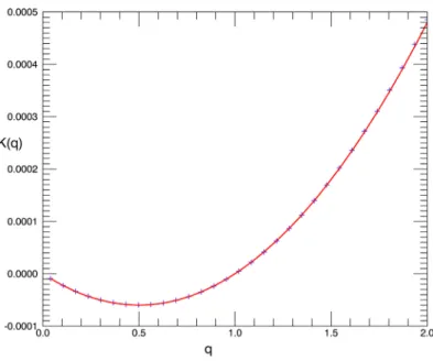
As mentioned in previous paragraphs, the moments scaling functionK(q) was calculated from slopes of lin-ear interpolations of the log-log curves (of different statistical momentsq). The universal multifractal (UM) fit (equation (6)) was calculated for the moments scaling function for the whole period 1998–2012. Example of the moments scaling functionK(q) and the UM fit are shown in the Figure 5 (SST in the Irish Sea for 2009). It was observed that the annual median SST data are, with very good approximation, described by the model of universal multifractals (equation (6)). The relative error of the UM fit was within 4%, but in most cases, it was less than 1%. The Table 1 shows the annual median data’sa,C1parameters (see equation
(6)) averaged through the period 1998–2012 with their fluctuationsDa5hja2haiji;DC15hjC12hC1iji. As
one can see in the Table 1,ais very close to the lognormal valuea52, but deviates from it a little bit. The
C1values obtained were of the order of 1024and fluctuated to some extent between years. One can further
see that interregional differences inaare very small and the dominant difference is inC1.
The same analysis was done for the annual median chlorophyll data. As for SST, the data showed consistency over different years. Again, only specific examples of the chlorophyll data can be pre-sented, for this purpose, the case of English Channel has been selected and is shown in Figure 6. As can be seen in Figure 6, in the English Channel, the 10 km scale appears to be a break point between two scaling regimes. This scaling property did not change over the years and was apparent even in the seasonal data. The annual median chloro-phyll scaling was well approxi-mated by multifractals: (i) for
Figure 3.The scaling of the annual median 2009 SST data statistical momentsq2 f0:2;2g for the Irish Sea.
Figure 4.The scaling of the annual median 2009 SST data statistical momentsq2 f0:2;2g for the Celtic Sea II region.
Brittany, from the 6 km scale to the maximum scale (80 km); (ii) for the Celtic Sea I and II, from the 8 km scale to 80 km scale; (iii) for the region around the Devon Coast, from 3–4.5 to 60–70 km, (v) as shown in Figure 6, the most interesting region was the English Channel region, where multifractal scaling is observed from approxi-mately 10 km scale up to the maximum scale (180 km). Wher-ever multifractal scaling was observed, the linear regression of the log-log plot had error within 8%. Particularly interesting was the Irish Sea region where there were extremely consistent annual patterns that could also be observed in the seasonal data. In the Irish Sea region, the chloro-phyll data showed no uniform scaling, but rather two separate scaling regimes: one on scales between 3 and 30 km and the other on scales 30 km to at least 140 km.
The UM fit for the chlorophyll data was worse than for SST, typically with a relative error between 5 and 10%. In the Celtic Sea I region, the relative error of the UM fit was much worse than in the remaining regions: it was between 10 and 20%. Thea,C1parameters are again shown in Table 2. As one can see in
Table 2,aparameter had always valuea52, implying a lognormal distribution. The interregional and inter-annual differences were obtained by different values ofC1.C1was for chlorophyll of the order of 1022in a
relatively narrow range of values, with the exception of Celtic Sea II region where it was 1 order of magni-tude lower. These lower values ofC1in the Celtic Sea II region naturally reflect the lower variability of
chlo-rophyll in this area. TheC1value for chlorophyll is 2–3 orders of magnitude larger thanC1for SST, which is a
consequence of chlorophyll being much more spatially heterogeneous than SST. This has been observed many times and explained in terms of the shorter characteristic response time of chlorophyll to the proc-esses that alter its concentrations [Mahadevan and Campbell, 2002, 2003;Mahadevan, 2004]. It is also inter-esting to point out that the interannual fluctuations displayed in Table 2 show that the chlorophyllC1
parameter fluctuated much less than the SSTC1parameter. Perhaps the reason for this was that there are
zero fluctuations ofaparameter for chlorophyll.
The option of using seasonal, rather than annual, field medians was investigated. For SST, the seasonal median data generally have less clear scaling properties than annual data. There are, however, some differences between seasons: it was observed over multiple years that the multifractal scaling is more pronounced for the spring and autumn seasons (the linear regression had the same error as for annual data), whereas it is less clear in the winter and summer sea-sons (for example, in Irish Sea, the error was 8–13%). The UM fit for both SST and chlorophyll and the seasonal data had approximately the same qual-ity as for the annual data. Thea
;C1 parameters fluctuate from
season to season but they remained within the same range as the annual median
Figure 5.The scaling moment functionK(q) for the annual 2009 SST in the Irish Sea region. The line is the UM fit of the points calculated from the slope of the linear regression.
Table 1.The UM Fit ParametersaandC1Calculated for 1998–2012 SST Annual Medians a
Region hai hC1i3105 Da DC13105
Bristol Channel 1.963 65 0.039 22
Brittany 1.971 27 0.032 14
Irish Sea 1.966 31 0.023 9
Celtic Sea 1.95 18 0.027 4
Celtic Sea II 1.949 13 0.029 5
Devon Coast 1.972 22 0.026 11
English Channel 1.976 16 0.021 6
a
The table shows averages ofaandC1through the period 1998–2012 as well as
values. For chlorophyll, the seasonal data have less clear patterns. How-ever, it is worth noting that in the English Chan-nel and Irish Sea regions, the chlorophyll seasonal and annual scalings are almost indistinguishable. This is especially true in the English Channel where pronounced scal-ing patterns exist from 10 to 14 km upward. To determine possible driving mechanisms for the surface heterogene-ity in both SST and chlo-rophyll, the scaling of the bathymetry was investi-gated. The bathymetry (B) incremental functions (DBq‘) scaling was well described by power laws in all the regions explored, on the scales from the order of kilometers to the scales>100 km. Again, power law in bathymetry incremental functions scaling (equation (8)) is observed as a straight line in log-log plots. An example is shown in Figure 8. The bathymetry increments scaling exponentHcan be easily determined from the linear regression of the logarithmic plots. TheHexponents were calculated, and their values can be found in Table 3. Note that the Table 3 does not contain the Celtic Sea II region, as there was lack of reliable bathymetry data in this region.
The annual and seasonal median data were also characterized using the increments scaling model (equation (8)). For most cases, clear multifractal scaling of the scalar increments function (Dqq‘) was appa-rent. For the annual median data, this can be seen in Figure 7. TheHvalues of the annual median data, shown in Table 3, were systematically calculated for both chlorophyll and SST for the period 1998–2012 (SST) and 1998–2004 (chlorophyll). The reason why shorter period was used for chlorophyll was lack of con-sistent data between 2005 and 2012. Table 3 shows 1998–2012 period averaged annual medianH(SST) and 1998–2004 averaged (chlorophyll) annual medianH. Table 3 also shows interannual fluctuations ofH meas-ured by a parameterhDHi5hjH2hHijicompared to the mean. For SST, there were couple of regions and years within which the multifractal scaling was not a good approximation and theHvalues from those years and regions were excluded. Table 3 shows that the SST meanHvalues are generally lower and fluctuate more than those for chlorophyll. It further shows that, as expected, the fluctuations between regions were larger than the fluctuations between years. The observed seasonal values ofHwere in the same range as the annual values (0.3–0.75) but sometimes showing mean interseasonal fluctuations as large as 20%. The single overpass imagery SST and chlorophyll increments were analyzed. The multifractal scaling was con-firmed in all the regions with an exception of chlorophyll in English Channel. In this specific case, a small scaling break appears around the 15 km scale. Interestingly, the break is (to a lesser extent) visible also in the annual profile and in the English Channel bathymetry data. As previously, only small selection of the results can be included in the paper; the scaling is demonstrated in Figure 9 on the example of ensemble-averaged space-time SST for the Celtic Sea II region. The H exponents are
Figure 6.The scaling of the annual median 2004 chlorophyll data statistical momentsq2 f0:2;2g in the English Channel region. Obvious multifractal scaling properties between 14 and 140 km can be seen.
Table 2.The UM Fit ParametersaandC1Calculated for 1998–2004 Chlorophyll
Annual Mediansa
Region hai hC1i3103 Da DC13103
Brittany 2 19.16 0 1.52
Celtic Sea 2 14.74 0 2.06
Celtic Sea II 2 3.26 0 0.45
Devon Coast 2 16.5 0 2
English Channel 2 16.13 0 1.69
a
The table shows averages ofaandC1through the period 1998–2004 as well
displayed in Table 4. It is worth noting that up to the maximal scale, no scaling breaks were observed. Such breaks could be associated with the flux homogeneity scale, which is the outer scale of the cascade process. The space-time fields scaling suggests that the outer scale is larger than the regional scales.
4. Discussion
In terms of oceanographic understanding, it is the physical interpretation of these statistics that is impor-tant. The space-time SST scaling exponents shown in Table 4 are significantly larger than expected for a passive scalar in a 3-D turbulence model. Since the horizontal dimensions are much larger than 1 km and the average depth is between 35 and 100 m, it is tempting to interpret these larger exponents as a transi-tion to the 2-D turbulent model. This has been observed inCurrie and Roff[2006]. This interpretation is sup-ported by the fact that the scaling exponent is largest in the shallowest coastal regions (Bristol Channel, Devon Coast) (see Table 4). The SST passive scalar value obtained in the literature [Seuront et al., 1996a, 1996b;Lovejoy et al., 2001b] has mostly matched well with the 3-D turbulence model (H50.3–0.42); how-ever, typically smaller scales were explored than in the present paper, scales in which 3-D turbulence model is expected to be a valid approximation. There is, however, an alternative (or additional) explanation for the steep SST profile: the tidal processes are very important in the shelf seas around British Isles and mixing by tidal currents can have a local homogenizing effect. Since such mixing will contribute differently in different spatial regions, it can effectively steepen the SST scaling profile. At present, we will not make a final state-ment on which of these two explanations is more plausible. As can be seen in Table 4, chlorophyll has less steep scaling profile than SST. This could be perhaps explained by the combined growth-passive scalar model [Lovejoy et al., 2001b] that has been suggested for phytoplankton scaling on scales larger than plank-tonscale (scale of the order of100 m at which zooplankton grazing is important).
The geographic distributions are quite different matter. The hypothesis from section 1 was confirmed in the sense that: (1) SST and chlorophyll scale on a large number of scales (submesoscale and mesoscale) as mul-tifractals. (2) Bathymetry shows multifractal scaling properties. It can be seen from Table 3 that chlorophyll geographic scaling exponents copy very well the scaling exponents of try. The dominant influence of bathyme-try results in the very low interannual fluctuations of the chlorophyll scaling exponent (227:5%). Chlorophyll produc-tion is dominantly affected by supply of nutrients to the surface and this is affected by the bathymetry and tidal currents. The main reason why bathyme-try scaling dominates chlorophyll, how-ever, may be the large differences between chlorophyll values near the coastline and in the regions further from the coast (chlorophyll is typically recorded on a logarithmic scale). SST also follows the bathymetry scaling pro-file (as anticipated), but with a much smaller scaling exponent (Table 3). This
Table 3.AveragedHof Median Chlorophyll (1998–2004) and SST (1998–2012), Compared With H of Bathymetrya
Region Hbath hHchlori DHchlor=hHchlori hHSSTi DHSST=hHSSTi
Devon Coast 0.934 0.868 7.35% 0.607 16.35%
Bristol Channel 0.909 0.506 12.96%
Brittany 0.821 0.755 3.15% 0.555 11.66%
Celtic Sea 0.627 0.679 2.11% 0.477 18.6%
English Channel 0.589 0.477 7.01% 0.507 11.09%
Irish Sea 0.514 0.498 2.73% 0.413 10.42%
a
The regions are ordered in terms ofHbath. The table also shows percent fluctuations of the Hexponent.
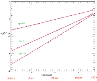
Figure 7.The scaling of the annual median 2004 chlorophyll data scalar incre-ments in the Celtic Sea. (Momentaq50:5;1;1:5.)
indicates the presence of another phenomenon, a phe-nomenon that is also responsi-ble for much larger interannual fluctuations of the scaling expo-nentH(10–19%). It is tempting to follow the hypothesis from section 1 and suggest that this is a combined effect of bathym-etry and bathymbathym-etry-induced inhomogeneities in turbulence. What the bathymetry-induced inhomogeneities mean is that, since the eddy formation proba-bility function is not translation-ally invariant, a turbulent profile remains to some extent in the time median data. The factor by which turbulent profile is affected by intermittency can be large if the eddies are very sparse. Since such traces of turbulence left in the annual median data are poten-tially very different from the ‘‘genuine’’ space-time turbulence (observed in the space-time SST profile), it is possible that eddy sparsity can effectively lower the value ofHSSTto the values observed in Table 3. However,
to move beyond this heuristic picture, it will be worth to construct a more precise (albeit simplifying) mathe-matical model relating the eddy formation probability to the bathymetry statistics. This will be a subject of the future work.
It is worth stressing that using multifractal techniques is a key element in obtaining these insights. The SST and chlorophyll-a profiles do not show any significant correlations in the regions analyzed (the effect of wind-driven upwelling is likely to be insignificant in these regions). Likewise, because of the effect of turbulence and large small-scale heterogeneity of multifractal distributions, it is expected that there is no significant spa-tial correlation between bathymetry and SST/chlorophyll. This means more direct statistical methods might say very little about the observed connections between SST, chlorophyll and bathymetry. On the other hand, theHincrements scaling parameter proves to be a very powerful tool for this type of analysis.
We have also shown that both SST and chlorophyll can be par-ameterized by couple of param-eters (universal multifractals). This has at least three significant implications: (1) the structures with multifractal scaling typically lead to singular measures, and are therefore relatively very het-erogeneous on small scales. Het-erogeneity then plays major role in any nonlinear phenomena: whenever nonlinearity is impor-tant, heterogeneity corrections to the results obtained from the fields mean values gain signifi-cance. The same holds true whenever spatial gradients become important. Any simple
Figure 8.The Celtic Sea: the scaling of the sea bottom topographyDDq‘whereDis the sea depth. (Momentaq50:5;1;1:5.)
Figure 9.The scaling of the overpass imagery data SST increments in Celtic Sea II region. (Momentaq50:5;1;1:5.)
heterogeneity parameterization can therefore be helpful when dealing with phenomena such as CO2 air-sea
exchange [Mahadevan, 2004]. (2) There is a second, very important application of the median data analysis: it presents a first step in developing a suitable metric to evalu-ate the numerical oceanographic model skill. Standard numerical model skill metrics compare observational and model data sets through statistical parameters such as corre-lation coefficient, root-mean-square error, average error, reli-ability index, and so on [Taylor, 2001; Doney et al., 2008;
Stow et al., 2009]. We suggest that multifractal parameters provide a particularly efficient way to structurally compare observational and model data sets. The simple statistics represented by the UM should be replicated by the model, resulting in a test for a model’s skill in reproducing spatial patterns. This skill evaluation metric, in addition to efficiency, has one significant advantage: because multifractal scaling carries important information about oceanographic drivers, a failure in the numerical oceanographic model’s ability to reproduce these scaling properties could automatically suggest which physical/biological parts of the model need better representation (or reparameterization). Therefore, the next step is to utilize these results and evaluate how numerical oceanographic models per-form in the shelf seas around the UK. (3) Third, if one were to extend these results to more global regions, UM parameterizations can potentially serve as a very efficient tool for data mining for large amounts of oceanographic data. In this context, one can also explore whether using generally scale-invariant aniso-tropic multifractal models that are nonself-similar [Schertzer and Lovejoy, 2011] significantly extends the number of observed scales of field scale invariance. Such anisotropic models already proven to be useful to model the scaling of the atmosphere on a large range of scales [Lovejoy et al., 2001a]. All these ideas are going to be a subject of future research.
References
Cates, M. E., and J. M. Deutsch (1987), Spatial correlations in multifractals,Phys. Rev. A,35, 4907(R).
Currie, W. J. S., and J. C. Roff (2006), Plankton are not passive tracers: Plankton in a turbulent environment,J. Geophys. Res.,111, C05S07, doi:10.1029/2005JC002967.
de Montera, L., M. Jouini, S. Verrier, S. Thiria, and M. Crepon (2011), Multifractal analysis of oceanic chlorophyll maps remotely sensed from space,Ocean Sci.,7, 219–229.
Doney, S. C., I. Lima, J. K. Moore, K. Lindsay, M. J. Behrenfeld, T. K. Westberry, N. Mahowald, D. M. Glover, and T. Takahashi (2008), Skill met-rics for confronting global upper ocean ecosystem-biogeochemistry models against field and remote sensing data,J. Mar. Syst.,76(1-2), 95–112.
Gagnon, J. S., S. Lovejoy, and D. Schertzer (2006), Multifractal earth topography,Nonlinear Processes Geophys.,13, 541–570.
Gurvitch, A. S., and A. M. Yaglom (1967), Breakdown of eddies and probability distributions for small-scale turbulence,Phys. Fluids,10, 59–65. Harte, D. (2001),Multifractals: Theory and Applications, Chapman and Hall, Boca Raton, Fla.
Kolmogorov, A. N. (1941), Local structure of turbulence in an incompressible liquid for very large Reynolds numbers,Proc. R. Soc. London, Ser. A,30, 299–303.
Landau, L. D., and E. Lifshitz (1963),Fluid Mechanics, Pergamon, N. Y.
Lavalee, D., S. Lovejoy, D. Schertzer, and P. Ladoy (1993), Nonlinear variability and landscape topography: Analysis and simulation, in Frac-tals in Geography, edited by L. deCola and N. Lam, pp. 171–205, Prentice Hall, N. J.
Lombardo, F., E. Volpi, D. Koutsoyiannis, and S. M. Papalexiou (2014), Just two moments! A cautionary note against use of high-order moments in multifractal models in hydrology,Hydrol. Earth Syst. Sci.,18, 243–255.
Lovejoy, S. (2014), A voyage through scales, a missing quadrillion and why the climate is not what you expect,Clim. Dyn.,44, 3187–3210. Lovejoy, S., and D. Schertzer (2010), Towards a new synthesis for atmospheric dynamics: Space-time cascades,Atmos. Res.,96, 1–52. Lovejoy, S., and D. Schertzer (2013),The Weather and Climate: Emergent Laws and Multifractal Cascades, Cambridge Univ. Press, Cambridge, U. K. Lovejoy, S., D. Schertzer, and J. D. Stanway (2001a), Direct evidence of ultifractal atmospheric cascades from planetary scales down to
1 km,Phys. Rev. Lett.,86(22), 5200–5203.
Lovejoy, S., W. J. S. Currie, Y. Tessier, M. R. Claereboudt, E. Bourget, J. C. Roff, and D. Schertzer (2001b), Universal multifractals and ocean patchiness: Phytoplankton, physical fields and coastal heterogeneity,J. Plankton Res.,23(2), 117–141.
Mahadevan, A. (2004), Spatial heterogeneity and its relation to processes in the upper ocean, inEcosystem Function in Heterogeneous Land-scapes, edited by G. M. Lovett et al., pp. 165–182, Springer, N. Y.
Mahadevan, A., and J. W. Campbell (2002), Biogeochemical patchiness at the sea surface,Geophys. Res. Lett.,29(19), 1926, doi:10.1029/ 2001GL014116.
Mahadevan, A., and J. W. Campbell (2003), Biogeochemical variability at the sea surface: How it is linked to process response times, in Handbook of Scaling Methods in Aquatic Ecology: Measurement, Analysis, Simulation, pp. 624, CRC Press, Boca Raton, Fla.
Mandelbrot, B. (1974), Intermittent turbulence in self-similar cascades: Divergence of high moments and dimension of the carrier,J. Fluid Mech.,62, 331–358.
Mandelbrot, B. (1982),The Fractal Geometry of Nature, W. H. Freeman, San Francisco, Calif. Mandelbrot, B. (1997),Fractals and Scaling in Finance, Springer, N. Y.
Table 4.TheHScaling Exponents of Ensemble-Averaged SST and Chlorophyll Single Overpass Imagery Data
Region hHSSTi hHchlori
Celtic Sea 0.652 0.485
Irish Sea 0.541 0.415
Devon Coast 0.771
Brittany 0.667
Celtic Sea II 0.672 0.538
English Channel 0.653 Bristol Channel 0.805
Acknowledgments
We would like to thank Ricardo Torres and Pierre Cazaneve for modeling discussions and providing the bathymetry data from Liverpool Coastal Observatory (POLCOMS high-resolution continental shelf model). We would also like to thank the NERC Earth Observation Data Acquisition and Analysis Service (NEODAAS) at the Plymouth Marine Laboratory for preparing all the median data for the analysis. The AVHRR, MODIS, and SeaWifs satellite single overpass imagery can be obtained free from NEODAAS (https://www.neodaas.ac. uk). The median data can also be obtained from NEODAAS upon request.
Martin, A. P. (2003), Phytoplankton patchiness: The role of lateral stirring and mixing,Prog. Oceanogr.,57, 125–174.
Nieves, V., C. Llebot, A. Turiel, J. Sole, E. Garcia-Ladona, M. Estrada, and D. Blasco (2007), Common turbulent signature in sea surface tem-perature and chlorophyll maps,Geophys. Res. Lett.,34, L23602, doi:10.1029/2007GL030823.
Novikov, E. A., and R. Stewart (1964), Intermittency of turbulence and spectrum of fluctuations in energy dissipation,Izv. Akad. Nauk SSSR, Ser. Fiz.,3, 408–412.
Obukhov, A. (1949), Structure of the temperature field in a turbulent flow,Izv. Akad. Nauk SSSR, Ser. Fiz.,13, 55–69.
O’Reilly, J. E., S. Maritorena, B. G. Mitchell, D. A. Siegel, K. L. Carder, S. A. Garver, M. Kahru, and C. McClain (1998), Ocean color chlorophyll algorithms for SeaWiFS,J. Geophys. Res.,103, 24,937–24,953.
Richardson, L. F. (1922),Weather Prediction by Numerical Processes, Cambridge Univ. Press, Cambridge, U. K.
Schertzer, D. (2013), Interactive comment on ‘‘Just two moments! A cautionary note against use of high-order moments in multifractal models in hydrology’’ by F. Lombardo et al.,Hydrol. Earth Syst. Sci. Discuss.,10, C3103–C3109.
Schertzer, D., and S. Lovejoy (1987), Physical modelling and analysis of rain and clouds by anisotropic scaling multiplicative processes, J. Geophys. Res.,92, 9693–9714, doi:10.1029/JD092iD08p09693.
Schertzer, D., and S. Lovejoy (1988), Multifractal simulations and analysis of clouds by multiplicative processes,Atmos. Res.,21, 337–361. Schertzer, D., and S. Lovejoy (1992), Hard and soft multifractal processes,Physica A,185, 187–194.
Schertzer, D., and S. Lovejoy (1997), Universal multifractals do exist!,J. Appl. Meteorol.,36, 1296–1303.
Schertzer, D., and S. Lovejoy (2011), Multifractals, generalized scale invariance and complexity in geophysics,Int. J. Bifurcation Chaos, 21(12), 3417–3456.
Schertzer, D., S. Lovejoy, and P. Hubert (2002), An introduction to stochastic multifractal fields, inISFMA, Symposium on Environmental Sci-ence and Engineering With Related Mathematical Problems, edited by A. Ern and W. Liu, pp. 106–179, High Educ. Press, Beijing. Schmitt, F., D. Schertzer, S. Lovejoy, and Y. Brunet (1993), Estimation of universal for atmospheric turbulent multifractal indices velocity
fields,Fractals,01, 568.
Seuront, L., and Y. Lagadeuc (1997), Characterization of space-time variability in stratified and mixed coastal waters (baie des Chaleurs, Quebec, Canada): Application to fractal theory,Mar. Ecol. Prog. Ser.,259, 81–85.
Seuront, L., and F. G. Schmitt (2005a), Multiscaling statistical procedures for the exploration of biophysical couplings in intermittent turbu-lence; Part I. Theory,Deep Sea Res., Part II,52, 1308–1324.
Seuront, L., and F. G. Schmitt (2005b), Multiscaling statistical procedures for the exploration of biophysical couplings in intermittent turbu-lence; Part II. Applications,Deep Sea Res., Part II,52, 1325–1343.
Seuront, L., F. Schmitt, Y. Lagadeuc, D. Schertzer, S. Lovejoy, and S. Frontier (1996a), Multifractal analysis of phytoplankton biomass and temperature in the ocean,Geophys. Res. Lett.,23, 3591–3594.
Seuront, L., F. Schmitt, D. Schertzer, Y. Lagadeuc, and S. Lovejoy (1996b), Multifractal intermittency of Eulerian and Lagrangian turbulence of ocean temperature and plankton fields,Nonlinear Processes Geophys.,3, 236–246.
Seuront, L., F. G. Schmitt, Y. Lagadeuc, D. Schertzer, and S. Lovejoy (1999), Universal multifractal analysis as a tool to characterize multiscale intermittent patterns: Example of phytoplankton distribution in turbulent coastal waters,J. Plankton Res.,21, 877–922.
Seuront, L., H. Yamazaki, and F. Schmitt (2005), Intermittency, inMarine Turbulence, edited by H. Baumert, J. Simpson, and J. Sundermann, pp. 66–79, Cambridge Univ. Press, Cambridge, U. K.
Siebesma, A. P., and L. Pietronero (1988), Correlations in multifractals,J. Phys. A Math. Gen.,21, 3259–3267.
Stow, C. A., J. Jolliff, D. J. McGillicuddy Jr., S. C. Doney, J. I. Allen, M. A. M. Friedrichs, K. A. Rose, and P. Wallhead (2009), Skill assessment for coupled biological/physical models of marine systems,J. Mar. Syst.,76, 4–15.
Taylor, K. E. (2001), Summarizing multiple aspects of model performance in a single diagram,J. Geophys. Res.,106, 7183–7192. Tel, T. (1988), Fractals, multifractals and thermodynamics,Naturforsch,43a, 1154–1174.
Yaglom, A. M. (1966), The influence on the fluctuation in energy dissipation on the shape of turbulent characteristics in the inertial interval, Sov. Phys. Dokl., Engl. Transl.,2, 26–30.