Sharif University of Technology
Scientia IranicaTransactions E: Industrial Engineering www.scientiairanica.com
Multi-objective sustainable supply chain with
deteriorating products and transportation options
under uncertain demand and backorder
M. Sepehri
and Z. Sazvar
Graduate School of Management and Economics, Sharif University of Technology, Tehran, Iran. Received 8 September 2014; received in revised form 28 June 2015; accepted 15 October 2016
KEYWORDS Sustainable supply chain;
Deteriorating products; Transportation; Possibilistic programming; Green supply.
Abstract. Supply chain sustainability, with economic, environmental, and social values, has gained attention in both academia and industry. For deteriorating and seasonal products, like fresh produce, the issues of timely supply and disposal of the deteriorated products are of great concern. This paper is to develop a possibilistic mathematical model, solved after linearizing the non-linear statements, and to propose a new replenishment policy for a centralized Sustainable Supply Chain (SSC) for deteriorating items. Dierent transportation vehicle options, which produce various pollution and greenhouse gas (GHG) levels, are considered. Several variables such as the end-customer demand, the partial backordered ratio, and the deterioration rate are uncertain. Deterioration occurs for in-stock inventories and during transportation. The solution provides the optimum transportation modes and routes, and the inventory policy by nding a balance between nancial, environmental, and social criteria.
© 2016 Sharif University of Technology. All rights reserved.
1. Introduction
\A supply chain is a system of organizations, people, technology, activities, information, and resources in-volved in moving a product or service from supplier to customer" [1]. Adding the `green' concept to the `supply chain' concept creates a new paradigm, where the supply chain will have a direct relation to the environment [2]. The green SCM concept is further developed into sustainable SCM to include social fea-tures of the supply chain as well as environmental and economic aspects.
There has been growing concern about the envi-ronmental and social footprints of business operations. People are conscious of the world's environmental problems, such as pollution, global warming, toxic
*. Corresponding author. Tel.: 021 66165856; Fax: 021 66022759
E-mail address: sepehri@sharif.edu (M. Sepehri)
substance usage, and non-renewable resources [2]. The majority of papers in supply chain network design focus on economic performance. Recent studies have considered environmental dimensions. There is a gap in quantitative models of social factors with environ-mental and economic impacts [3].
Uncertainty is an inherent attribute of supply chains, which aects the supply chain's performance and complexity. Numerous methods exist for quan-titative description of supply chain uncertainty in the literature, most generally involving interval analysis [4], possibilistic and fuzzy sets methods [5], stochastic programming methods [6], etc.
Transportation is a major factor in deteriorating products supply chain, as deterioration and economic and environmental factors depend on the distance and condition of product transportation. To reduce purchase costs and attract a larger base of customers, retailers, such as WalMart, Home Depot, and Costco, are constantly seeking suppliers with lower prices and
nding them at greater distances from their distribu-tion centers and stores [7].
This paper employs many of the recent aspects of deteriorating products SCM. It simultaneously con-siders economic, environmental, and social objectives; transportation and route options; uncertain demand; deterioration and backorder ratios; and non-linear sale price discount. Deterioration can occur both in in-stock inventories and during transportation in the model. Deterioration during transportation is a function of transportation type (truck vs. airplane, refrigerated vs. individually packed, etc.) and transportation routes. A possibilistic approach is used to nd the optimum solution for a centralized supply chain, where the leftover product is disposed of for a given amount of cost or prot. These distinct features are used simultaneously to provide a holistic model and reach an applied solution. The main research question is the impact of the social factors introduced in the model, combined with the economic and environmental impacts. A fresh produce center in Tehran, Iran, was used to gather data and test the model.
In the next two sections, various relevant aspects of SCM used in our research, i.e. Sustainable Sup-ply Chains (SSC), deteriorating products, and fresh produce, are reviewed. Section 4 presents the prob-lem description, including notations and assumptions, followed by the sections on the mathematical model, solution approach, numerical analysis, and conclusions.
2. Literature review
The literature review is presented in two sub-sections: We rst review some of the main studies on SSC, and then assess some major research on replenishment policies for deteriorating products.
2.1. Sustainable supply chain
The Brundtland Report [8] underlined the importance of sustainable development and called for \a better life for everyone without destroying the natural resources for future generations". Since then, the concept of sustainability has been broadened to include Planet, People, and Prot [9]. It may be argued that \Sustain-able Development" and \Sustainability" are not essen-tially the same. Accordingly, the former is concerned with processes while the latter is considered as a state. These two terms are frequently used interchangeably in the literature without highlighting the dierences [10]. In this paper and most other studies in the supply chain literature, the concept used is sustainability.
Organizations are increasingly assimilating sus-tainability into their SCM practices. Although the motivations of individual organizations may vary, key objectives generally include an interest in achieving sustainable streams of products, services, information,
and funds to provide maximum value for involved stakeholders [11].
According to [12], Sustainable SCM (SSCM) is \the management of material, information, and capital ows as well as cooperation among companies along the supply chain while integrating goals from all three dimensions of sustainable development, i.e., economic, environmental, and social, which are derived from customer and stakeholder requirements."
Table 1 shows an illustrative sample of recent papers in the area of SSC. While this is by no means a representative sample of all existing research in the literature, it is sucient to illustrate the gaps and deciencies in the current research. For a more comprehensive review of studies in the eld of SSCs, interested readers are referred to [13]. According to Table 1, the related literature can be characterized in three groups based on the direction of material ows:
i) Forward Logistic (FL): Many researchers have considered the sustainability concept in forward logistic processes (conventional logistic) where af-ter procuring from suppliers, raw maaf-terials are converted to nished goods at manufacturer sites and, subsequently, transferred to customers via distribution centers to fulll their demands [14]. Brandenburg et al. [13] provide a review of 134 pa-pers on quantitative, formal models that addressed sustainability aspects in forward supply chains;
ii) Reverse Logistic (RL)/Backward Logistics (BL): These studies consider the ow of used or returned products from the customers back to the collection centers for reusing, remanufacturing, recovering, disposal, etc;
iii) Closed-loop supply chains: These studies, such as [3,5,15], consider a supply chain network by inte-grating the forward processes with the backward processes.
In addition, many SSCM quantitative models developed for uncertain conditions come from various sources like demand, capacities, costs, etc. Based on Sazvar et al. [6], there are four main approaches for considering uncertainty in the decision-making process: robust optimization, stochastic programming, fuzzy programming, and stochastic dynamic programming.
As Table 1 shows, very few studies take into ac-count multiple sustainability dimensions as compared to studies developed in green supply chains (consider-ing economic and environmental criteria). Many stud-ies present real-world cases from the pharmaceutical, medical, glass, food, etc. industries to demonstrate the applicability of their developed models. However, limited research has explicitly addressed an important category of products called deteriorating items. In the
Table 1. Illustrative sample of research on sustainable replenishment. Year Author(s) Modelling
approach
Characteristics: Forward/ backward
Application in real cases
Uncertain parameters
Economic criteria
Environ. criteria
Social criteria
2010 Pishvaee Torabi & [5]
Possibilistic prog.
Forward/
backward |
Costs, capacities,
demands, rates of return products
Min total
costs {
Total delivery tardiness
2014 Validi et al. [20]
Mixed integer prog.
Forward Food
industry |
Min total costs
Min. CO2 emission
2011 Pishvaee, et al. [21]
Robust possibilistic
prog.
Forward Medical industry
Costs, demand, capacities
Min total
costs |
Max social responsibility 2014 Sazvar
et al. [6]
2-stage stock prog.
Forward Pharmaceutical
industry Demand
Min total costs
Min. GHG
emission |
2011 Wang et al. [22]
Mixed integer prog.
Forward A procurement
center |
Min total cost
Min. CO2
emission |
2015
Das and Posinasetti
[15]
Mixed integer program, goal prog.
Forward/
backward |
Returned products to the
retailer (scenario
based)
Max total prot
1-min. spent energy -Min.
harmful emission
|
2010 El-Sayed et al. [23]
Multi-stage stochastic
prog.
Forward/
backward | Demand
Max total
prot | |
2014 Devika et al. [3]
Mixed integer prog.
Forward/ backward
Glass
industry |
Min total costs
Min. CO2 emission
Max social responsibility
2010 Jamshidi et al. [24]
Mixed Integer Prog.
Forward | Demand Min total
costs
Min produced dangerous gases (NO2, CO, volatile
organic (VOCs))
|
next sub-section, in Table 2, the literature on these types of products is reviewed.
2.2. Deteriorating products
Deterioration of goods is a common phenomenon. Pharmaceuticals, blood, owers, fruits, vegetables, dairy, meat, and foods are just a few examples. Perishable models have been widely studied in recent years. The literature on perishable product SCM has
skyrocketed. Deterioration is dened as the damage, spoilage, vaporization, dryness, etc. of items [16]. Continuously deteriorating items suer loss in quantity or in quality. This is distinct from obsolescence, or sudden death, where items lose their value because of rapid change in technology, introduction of a new product, or going out of fashion [17]. Ghare and Schrader [16] were among the rst to study deteri-orating products and developed an inventory model
Table 2. Illustrative sample of research on deteriorating products replenishment.
Year Author Solution approach
Demand function
Deterioration function
Inventory system
Shortage PB: partial backorder
Planning horizon
Objective function 2014 Kim
et al. [26] Exact-simulation Constant Inventory dependent FOQ Backorder Innite Min cost 2011 Wang
et al. [33] Heuristic Constant Time dependent FOQ/FOI NO Innite Min cost 2011 Wee
et al. [34] Exact Constant Constant FOQ/FOI NO Finite Max prot
2010 He
et al. [35] Exact
Time
dependent Constant FOQ/FOI NO Finite Min cost
2009 Wee and
Chung [36] Exact Constant Constant FOI NO Innite Min cost
2008 Liao [37] Exact Constant Constant FOQ NO Innite Min cost
2008 Urban [38] Heuristic Inventory dependent
Non-linear time dependent
holding cost
FOQ/FOI NO Innite Max prot
2007 Dye [39] Heuristic Price
dependent Time dependent FOQ P.B Innite Max prot
2007 Mahata &
Goswam [40] Exact
A fuzzy number
A constant deterioration rate + A fuzzy
holding cost
FOI NO Innite Min cost
2005 Dye &
Ouyang [41] Exact
Inventory
dependent Constant FOI/FOQ P.B. Innite Max prot 1998 Luo [42] Numerical
Price and advertisement
dependent
Weibull FOQ Lost sale Innite Max prot
1982 Weiss [43] Exact 1- Constant, 2-Poisson
Non-linear time dependent
holding cost
FOQ/FOI NO Innite Min cost
for exponentially decaying inventory. Amorim et al. [18] studied the eects of concurrent optimization of production and distribution for perishable products. Prastacos [19] published a survey of blood inventory management.
Bakker et al. [25] reviewed over 200 papers pub-lished in the last decade on deteriorating inventory systems. In Table 2, a summary of the main re-lated research is presented. The types of demand, shortage, and deterioration functions for each study are reported. More details about some of the main assumptions, such as inventory system (Fixed Order
Quantity (FOQ)/Fixed Order Interval (FOI)), solution approach, planning horizon, and objective function types are also presented.
From Tables 1 and 2, it can be seen that little research deals with deteriorating products in SSCs in comparison with the research on products with unlimited lifetime. Sazvar et al. [6] developed a stochastic replenishment model in a centralized green supply chain for deteriorating items, with inventory and transportation costs and the environmental impact under uncertain demand. They found, because of the recycling of deteriorated items, the environmental
impact of deteriorating items was more signicant than that of non-deteriorating ones. Kim et al. [26] studied a closed-loop supply chain where Returnable Transport Items (RTIs) were applied to ship deteriorating goods from the supplier to the buyer. Then, empty RTIs were collected at the buyers and returned to the supplier.
In summary, the main issues, like considering social criteria, deterioration during transportation, and eect of transportation paths, as well as vehicle types on deterioration process, are signicantly challenging in the real world. However, to the best of our knowledge, less attention has been paid to quantitative studies. 2.2.1. Fresh produce
Fresh produce (fruits, owers, and vegetables) is a fast growing segment of the economy, and exporting and importing of fresh produce are common phenom-ena [27]. The success factors in fresh produce SCM include continuous investment (despite tight margins), volume growth (providing condence in the future), improvement of measurement and control of costs (in the pursuit of gains in eciency), and innovation (the level of service and the way of doing business with key customers) [28].
The challenge in managing fresh produce is that product value deteriorates signicantly over time at rates that are highly temperature- and humidity-dependent. The scope of most published studies is the post-harvest supply chain [38]. Agricultural issues like seed production and growing have not been explored. A decision about supply chain involves a choice between responsiveness and eciency [28]. Blackburn et al. [29] found that supply chain should be responsive in the early stages and ecient in later stages.
For fresh produce, a retailer procures from a supplier a quantity of a fresh product, which must then be transported to reach the target market. The retailer has to make an appropriate eort to preserve freshness of the product, and may pay higher costs for better transportation [28]. In practice, it is common to oer deteriorated items at a discount price. In supermar-kets, items near the expiration date are marked down to inuence buying behavior the consumer [30].
Shukla and Jharkharia [31] presented a literature review of the fresh produce SCM, with processes from production to consumption. The main interest in fresh produce SCM is consumer satisfaction and revenue maximization, while post-harvest waste reduction is a secondary objective. Inaccuracy in demand forecast-ing, demand and supply mismatch, lesser integrated approach, etc. are of concern. Though social and environmental factors in fresh produce supply chain are major concerns, very little research exists at this time on developing a comprehensive SSCM model for these products.
3. Research gaps
Worldwide grocery retailers' sales in 2012 exceeded $1,000 billion. Deteriorating products, such as fresh produce, dairy, and meat, account for more than a third of these sales [32]. Managing SCM of deteriorating products is progressively becoming more important. Today's customers request greater product diversity and price. Thus, more deteriorating products tend to exceed the best-before date, while demand and price per product tend to be less predictable. In addition to normal SCM costs (ordering, transportation, holding, and shortage), deteriorating items impose extra costs on the system.
Today, for many corporations, sustainability is a major factor for competitiveness and survival. The environmental factors, for deteriorating product man-ufacturers and retailers, not only come from trans-portation factors and GHG emissions, but also are a factor of disposal of spoiled and unused products. The social factors need to be considered equally and separately as parts of sustainability, too. Social factors, in particular for seasonal and highly volatile demand products, are becoming strategic issues. Firms can no longer easily hire and re employees at will, ignore their welfare and training, impose unreasonable hours and working conditions, etc. For products traded multi-nationally, local workers need specic treatment, by law and by social responsibility principles, so that work would not be sent oshore just because of cost or trade considerations. For deteriorating products, such as fresh produce, there is a mismatch between supply and demand, encouraging increasing imports and exports.
The motivation for this research comes not only from a lack of suitable work in the literature, but also from the growing importance of the above gaps in practice. Deteriorating items increasingly aect the lives of employers and consumers in the developed and developing countries, and are exceedingly creating issues in economic, environmental, and social fronts for corporations and politicians.
This research considers the sustainable supply chain planning problem for deteriorating products in a multi-period environment under: i) uncertain demand and ii) a price-discount scheme, and by considering iii) sustainability criteria, particularly social and human-resource related ones; iv) dierent transportation vehi-cle types as well as dependency of on-the-way deterio-ration rate to the vehicle types; v) dierent paths for transportation depending on on-the-way deterioration rate to the path types; and vi) various costs such as shortage, disposal, and human resource costs.
Reviewing the existing literature shows that though a great deal of research has been conducted on these types of problems, to the best of our knowledge, no holistic system has been developed to cover all
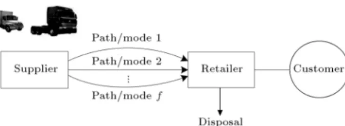
Figure 1. A schematic of the considered supply chain.
aspects of the above description. A broad range of such studies has been devoted to some of its aspects separately or to their specic combinations. Therefore, there is a gap between practical and theoretical contri-butions of deteriorating product's SCM, and the aim of this paper is to bridge this gap by considering all the mentioned aspects in a centralized SSC.
4. Problem description
A centralized forward supply chain provides a deteri-orating product, as shown in Figure 1. The supply chain consists of three kinds of entities: a supplier, a retailer, and customers. The planning horizon is nite and consists of multiple periods. At each period, a quantity order is supplied by the supplier and shipped to the retailer in order to respond to end-customer's demand. Because of deterioration characteristics of the product, if inventory is left at the end of a period at the retailer site, ~ percent of it should be disposed. The end-customer's demand ( ~D) and deterioration rate of on-hand inventories (~) are considered as uncertain parameters.
Since the demand rate ( ~D) and deterioration rate (~) are uncertain, shortage can occur at each period, which may be partially backordered. In this way, at each period, ~ ratio of unfullled demands (if exists) can wait up to the next period, while the other 1 ~ ratio will be lost. ~ is assumed to be uncertain, too.
The supplier, providing the product, should ship it to the retailer. There are several transportation vehicle options available at the supplier site. Each one is characterized by its capacity, transportation cost, GHG emission, and the deterioration of on-the-way product. Each type of transportation vehicles has its technical specications, which aect the product deterioration rate during transportation. Thus, the deterioration rate of on-the-way product is variable and depends on the vehicle type.
As in Figure 1, there are also various paths (or transportation modes) from the supplier to the retailer. In the real world, various types of vehicle and dierent paths are available to send goods from suppliers to retailers. The vehicle types/paths have a considerable inuence on each product's transportation cost, amount of GHG emission, and deterioration rate of product. For example:
More modern and ecient transportation vehicles keep the product healthier and generate less GHG, but they incur higher costs;
Sometimes, transportation by ship is faster and cheaper, but results in more disposals because of humidity. In contrast, overland paths cause fewer disposals, but are more expensive and slower;
Sometimes, using vans is more rapid and more ex-pensive, and thus, it results in low product disposal in comparison with using trucks.
In summary, there are two sources of deterio-ration: i) deterioration rate of on-hand inventory at retailer warehouse (~) and ii) deterioration rate of on-the-way products (~vf), which is aected by vehicles
type (v) as well as transportation paths/mode features (f).
In many real cases, the selling price depends on the sale quantity. In this problem, the selling price (pr) is non-linearly dependent on the sale quantity by the following function:
pr = 8 > > > < > > > :
pr1 SA0 St< SA1
pr2 SA1 St< SA2
::: :::
prm SAm 1 St< SAm
(1)
In Eq. (1), St indicates sale in period t. Also, pr1 >
pr2 > pr3 > ::: > prm > 0 and SA0< SA1< SA2 <
::: < SAm are positive parameters. In other words, as
the sale-quantity increases, the selling price decreases. The objective is to nd the best conguration of vehicle type, transportation path/mode, and order quantities in each period to simultaneously meet the following criteria:
i) Maximizing the total prot (an economic objec-tive);
ii) Minimizing total GHG emissions (an environmen-tal objective); and
iii) Minimizing human recourse variations from one period to another (a social objective).
There is a need for employees to carry out the logistic activities, including transportation and other logistic activities, throughout the supply chain. In some periods, since the forecasted customer demand is very high, the order quantity and, consequently, the amount of required logistic activities throughout the chain increase in order to respond to demand. These logistic activities are packing products at the supplier, unpacking products at the retailer, repacking products at the retailer, issuing invoices, etc. The required transportation eet and, thus, the labor needed may also increase. In such periods, usually, the number of
required workers is more than the number of workers available in the supply chain. In this way, either some extra labor must be hired or the supply chain managers accept leaving a part of the demands unsat-ised.
In contrast, in some periods, the forecasted de-mand is very low and, as a result, the order quantity and the volume of required logistic activities decrease in comparison with the previous periods. In such periods, the supply chain managers decide either to keep a number of workers inactivated or to re them. In the production planning literature, adjusting resource levels (including human resources) to the volume of forecasted demands is called \chase strategy". Some disadvantages of this strategy are reducing job interest, decreasing the job satisfaction and job security of workers, and increasing administrative costs related to high levels of hiring and ring. In this way, variations in labor levels from one period to another can be regarded as a signicant social criterion in supply chains.
The opposite of chase strategy is \leveling strat-egy" where a xed number of workers are kept through all periods regardless of changes in the forecasted demands. A main disadvantage of this strategy is high level of inactivated workers in some periods. Usually, the optimal strategy is somewhere between \chase strategy" and \leveling strategy", which can be determined by the mathematical model developed in this paper by considering economic, environmental, and social criteria.
4.1. Assumptions
The following assumptions are also considered in de-veloping the proposed mathematical model:
The uncertain parameters, ~D, ~, ~, and ~vf, are
fuzzy numbers;
The retailer's initial inventory (or shortage) level, I0
(or B0), can be positive, zero, or negative;
Human resource level consists of two components: i) required human resource for transportation, called \transportation labors", and ii) required human resource for doing other logistic activities (except transportation) through the supply chain, such as packing products at supplier, unpacking and repack-ing products at the retailer, etc. We have called these labors \logistic labors";
Purchase cost (c), holding cost (h), backorder cost (), lost sale cost (), and disposal cost (SV ) for a unit of product are given and xed parameters;
There is a limited number of vehicles of each type;
The cost of disposal for each unit of product, SV , is dened by a multiple-breakpoint function as follows:
SV = 8 > > > < > > > :
SV1 K0 disposal quantity < K1
SV2 K1 disposal quantity < K2
::: :::
SVp Kp 1 disposal quantity < Kp
(2)
In the above function, each SVi (0 i p) is a
predened parameter that can be positive, negative, or zero depending on the case. For example, deteri-orated plastics or drugs are usually sold to recycling centers and, therefore, bring money for the system. In contrast, deteriorated fruits and vegetables have to be disposed, which is cost-generating. K0 <
K1 < K2 < ::: < Kp are positive parameters.
Finally, in Eq. (2), \disposal quantity" refers to two sources: i) on-hand inventories deteriorated in each period; and ii) on-the-way products deteriorated in each period.
4.2. Notations
The following notations are applied to develop the proposed model:
Indices
t Index of time period, t 2 f1; :::; T g v Index of transportation type,
v 2 f1; :::; V g
f Index of path from supplier to retailer, f 2 f1; :::; F g
m Index of sale quantity level, m 2 f1; :::; Mg
p Index of disposal level, p 2 f1; :::; P g General parameters
T Planning horizon length ~ Deterioration rate of in-stock
inventories
~ Fraction of demand backordered during a stock-out
~
Dt Demand in period t
df Distance between supplier and retailer
under path/mode f
CAPv Capacity of a type-v vehicle (dened
by unit of product)
MAXTv Maximum number of type-v vehicles
available
~vf Deterioration rate of product when
it is transported by a type-v vehicle through path/mode f
Economic parameters
O Fixed ordering cost for each replenishment
OCt Ordering cost in period t
pr A product unit selling price
h A product unit holding cost per period Penalty cost of a product unit lost sale
(including lost prot)
Backordered cost of a product unit per period
SV Disposal cost (or income) of a product unit
T Avf Cost of transportation by a type-v
vehicle for each unit of distance through path/mode f
Environmental parameters
Gvf GHG emission level produced by a
type-v vehicle under path f
GD GHG emission level produced by a unit of disposed product
Social parameters
HTv Required labor for using a type-v
vehicle
HUM Average number of products in each period for which a worker can do the related logistic activities (excluding transportation) and prepare them to deliver to the customers
Decision variables
It Inventory level at the end of period t
Bt Shortage level at the end of period t
Qt Net order quantity of period t received
by retailer
tvf Gross order quantity of period t
transported by a type-v vehicle through path f
t On-the-way inventories deteriorated in
period t
Xtvf Number of type-v vehicles used in path
f in period t
HUt Number of labors required in period t
St Total sale in period t
Z1 Total cost of the supply chain
Z2 Total GHG produced in the supply
chain
Z3 Total variations in human resource
5. Mathematical model
The proposed mathematical model is developed in two steps: First, it is developed in a non-linear form, and second, the equivalent linear form of the non-linear mathematical model in the previous step is developed by applying some linearization techniques.
5.1. Non-linear mathematical model
In terms of the above assumptions and notations, the proposed model can be formulated as follows:
MaxZ1=
X
t>0
pr:St
X
t>0
(OCt+ C:
X
v;f
tvf+ h:It
+ (1 ~)::Bt+ ~::Bt
+X
v;f
(T Avf:df:Xtvf)
+ SV:(~:It+ t)) + CHt:HUt
; (3)
MinZ2=
X
t>0
0 @X
v;f
(Gvf:df:Xtvf)+GD:(~:It+t)
1 A ;
(4)
MinZ3=
X
t
HU
t HU(t 1)+X t;v
HTv:X f
Xtvf
X
f
X(t 1)vf
; (5)
s.t.
Qt+ (1 ~):I(t 1) D~t ~:B(t 1)= It Bt 8t;
(6) It:Bt= 0 8t; (7)
OCt=
(
O Qt> 0
0 otherwise 8t (8)
t=
X
v;f
~:tvf 8t; (9)
Qt=
X
v;f
(1 ~vf):tvf 8t; (10)
(HUt 1)
P
v;ftvf
HUM HUt 8t; (11) X
v;f
tvf
X
v;f
CAPv:Xtvf 8t; (12)
X
f
Xtvf MAXTv 8v; t; (13)
Xtvf; HUt 0; integer 8t; v; f; (14)
Eq. (3) represents total prot, which is total rev-enue minus total cost. To calculate total revrev-enue (Pt>0pr:St), the product selling price, pr, is dened
based on Eq. (1). The total cost of system consists of ordering, procurement, holding, lost sale, backordering, transportation, disposal costs, and the wage of logistics worker, respectively. Without losing generality, it is assumed that the wages of the transportation worker are included in transportation costs of vehicles (T Avf).
As mentioned above, disposal cost consists of two parts: cost/income of on-hand inventories deteriorated (~:It)
and cost/income of on-the-way inventories deteriorated (Pv;f~vf:tvf). Moreover, a product unit disposal
cost, SV , follows the multiple-breakpoint function dened by Eq. (2).
Eq. (4) represents the environmental goal, which is minimization of total GHG emission from the supply chain. It consists of GHG emitted by transportation, deterioration of on-hand inventories, and deterioration of on-the-way inventories, respectively.
Eq. (5) is related to minimization of the total vari-ation in the labor level from one period to another. It consists of two terms, variation in the required level of logistics and transportation workers, respectively. This equation is considered as a social objective function. As mentioned, changes in labor levels from one period to another not only explicitly aect costs of systems (due to the costs of hiring, ring, etc), but also have implicit and negative eects on job satisfaction, well-being, and loyalty of personnel. Dening Z2 and Z3 along
with Z1 leads to an economic ordering policy, which is
compatible with the two main criteria of sustainability, i.e. minimization of GHG emissions (an environmental index) and labor level variations (a social index).
Constraint (6) is the inventory balance equation. Since the on-hand inventories deteriorate at rate ~, in Eq. (6), the initial inventory of period t is regarded as (1 ~):I(t 1). Also, ~ percent of the unfullled demand
(shortage) in period (t 1) is transferred to period t, which in Eq. (6) is regarded as part of that period's requirements. Constraint (7) implies that inventory and shortage levels of each period cannot take positive values concurrently. Since the ordering cost is incurred when the order quantity is positive, Constraint (8) is dened. Constraint (9) represents the equation for the on-the-way deteriorated inventories in each period. Constraint (10) means that order quantity in each period is the sum of non-perished products delivered by all transportation vehicles. Constraint (11) is dened to determine the number of required logistics workers in period t, HUt. According to this constraint,
the gross order quantity of each period, Pv;ftvf, is
divided by HUM. The quotient is then rounded up to determine how many workers are needed to handle logistic activities (excluding transportation) at period t, i.e. HUt. In this way, Constraint (11) explicitly and
other constraints, including decision variables, tvf,
implicitly aect the social criterion (Z3).
Constraint (12) guarantees that the quantity transported by vehicles is less than or equal to vehicle capacity. Constraint (13) shows the number of used type-v vehicles is less than or equal to the available type-v vehicles. Constraints (14) and (15) dene variable types.
5.2. Equivalent linear mathematical model There are several nonlinear expressions in the model developed above. In this section, we develop an equiv-alent linear mathematical model by applying some lin-earization techniques to nd global optimum solutions by the help of some optimization packages. As stated in Section 5.1., Constraint (7) implies that It and Bt
cannot be positive values concurrently. Constraint (7) can be converted to its equivalent linear form by the following two constraints:
Bt M:Nt 8t; (16)
It M:(1 Nt) 8t; (17)
where, in Eqs.(16) and (17), Nt; t = 1; :::; T are binary
variables as follows: Nt=
(
1 It= 0
0 Bt= 08t (18)
Generally, an ordering cost (O) is incurred in a period if the order quantity at that period is positive, as in Constraint (8). The ordering cost at period t can be stated as linear expression, O:Vt, where Vt are binary
variables and the following constraint holds: Vt
M Qt M:Vt: (19) In Constraint (19), the binary variables, O:Vt, are equal
to 1 if Qt> 0, and 0 otherwise:
Vt=
(
1 Qt> 0
0 Qt= 08t (20)
The total sale in period t and St is as Eq. (21). In
other words, the total sale is equal to the minimum amount of requirements (Dt+ ~:B(t 1)) and inventories
(Qt+ (1 ~):I(t 1)) as follows:
St= min
n
Qt+ (1 ~):I(t 1); ~Dt+ ~:B(t 1)
o
= 8 > > > < > > > :
Qt+(1 ~):I(t 1); ~Dt+ ~:B(t 1) Qt
+(1 ~):I(t 1)
~
Dt+ ~:B(t 1); D~t+ ~:B(t 1)< Qt
+(1 ~):I(t 1)
(21)
The linearization process of total sale is implemented in three steps.
Step 1: At this step, we dene binary variables, Ytand non-negative variables Q0t and Q00t. By these
variables, Eq. (21) is transformed into Eq. (22): St=Q0t+ (1 ~):I(t 1):Yt+ ( ~Dt+ ~:B(t 1))
:(1 Yt) 8t; (22)
where the following constraints must be added to the main model:
Q0 t
~
Dt+ ~:B(t 1) (1 ~):I(t 1)
:Yt 8t; (23)
~
Dt+ ~:B(t 1) (1 ~):I(t 1)
:(1 Yt)
Q00
t M:(1 Yt) 8t; (24)
Q0
t+ Q00t = Qt 8t: (25)
Step 2: To transform the product terms I(t 1):Yt
and B(t 1):Yt (in Eqs. (22)-(24)) into linear terms,
two non-negative variables ftand wtare introduced,
where ft = I(t 1):Yt and wt = B(t 1):Yt. Thus,
Eqs. (22)-(24) are replaced by Eqs. (26)-(28) as follows:
St= Q0t+ (1 ~):ft+ ~Dt:(1 Yt) + ~:B(t 1)
~:wt 8t; (26)
Q0
t ~Dt:Yt+ ~:wt (1 ~):ft 8t; (27)
(1 Yt): ~Dt+ ~:B(t 1) ~:wt (1 ~)
:I(t 1)+(1 ~):ftQ00tM:(1 Yt) 8t:
(28) The non-linear equation ft = I(t 1):Yt can also be
replaced by the following two linear equations: Yt:M ft Yt:M 8t; (29)
I(t 1) (1 Yt):M ft I(t 1)+(1 Yt):M 8t:
(30) Equation wt= B(t 1):Ytis similarly substituted by
linear Constraints (31) and (32):
Yt:M wt Yt:M 8n; (31)
B(t 1) (1 Yt):M wt B(t 1)+(1 Yt):M 8t:
(32) According to these two steps, the total sale at period t, Stcan be stated as a linear expression (Eq. (26)).
In this way, some extra variables (Yt; Q0t; Q00t; ft; wt)
and constraints (Eqs. (25)-(32)) are added into the main model.
The total revenue at period t is indicated by Rt. It is obtained by selling price (pr) times total
sale (St), i.e. Rt = pr:St. Thus, if the selling price
of product (pr) is a constant parameter, the total revenue at period t (pr:St) is linear. However, in
our problem, the selling price of product (pr) is quantity-dependent following Eq. (1). Thus, the total revenue at period t is as follows:
Rt= pr:St=
8 > > > < > > > :
pr1:St SA0 St< SA1
pr2:St SA1 St< SA2
::: :::
prm:St SAm 1 St< SAm
8t (33)
where St is expressed in Eq. (26). The next step
is therefore dened to develop the equivalent linear expression for the above multiple-breakpoint total revenue function.
Step 3: To formulate Eq. (33) as a linear ex-pression, we dene binary variables, ttm and
non-negative variables, SLtm. Then, Constraints
(34)-(36) are added as follows:
SAm 1:ttk SLtm SAm:ttm 8m; t; (34)
St=
X
m
SLtm 8t; (35)
X
m
ttm= 1 8t: (36)
The total revenue at period t(Rt) can
there-fore be formulated as a linear expression, Rt =
P
mprm:SLtm:
Another linearization process is related to dis-posal cost. As mentioned, the disdis-posal cost of each unit of product follows a multiple-breakpoint function as stated in Eq. (2). The disposal cost can therefore become linear by using the technique applied in Step 3 of revenue linearization process. In this way, non-negative variables, ILtp, and binary
variables, tp, are dened, where t 2 f1; :::; T g
and p 2 f1; :::; P g. Then, the following constraints should be added to the model:
Kp 1:tp ~:ILtp Kp:tp 8p; t; (37)
It=
X
p
ILtp 8t; (38)
X
p
tp= 1 8t: (39)
In this way, the disposal cost of deteriorated on-hand inventories can be stated by the linear
expres-sion PtPpSVp:~:ILtp. In a similar way, disposal
cost of on-the-way inventories is stated by linear expressions. t represents on-the-way inventories
deteriorated in period t, i.e. t = Pv;f ~:tvf.
By dening binary variables, 0
tp, non-negative
vari-ables, Ltp, and Constraints (40)-(42), total
dis-posal costs of on-the-way inventories can be stated asPtPpSVp:Ltp:
Kp 1:0tp Ltp Kp:0tp 8p; t; (40)
t=
X
p
Ltp 8t; (41)
X
p
0
tp= 1 8t: (42)
When an order is received by the retailer, non-deteriorated products are isolated from non-deteriorated ones. In this way, deteriorated on-the-way inven-tories are disposed at the beginning of the periods while disposing of deteriorated on-hand inventories is done at the end of each period. In other words, disposing of deteriorated on-the-way inventories and deteriorated on-hand products are is carried out at the same time. This is why we separate the linearization procedure of these two processes' costs. With some minor modications, the developed mathematical model can also be applicable when these two processes are done concurrently.
Finally, the last non-linear expression in the mathematical model developed in Section 5.1. is related to Z3 (Eq. (5)) including absolute terms.
The term jHUt HU(t 1)j could be converted to
a linear one with the help of two non-negative auxiliary variables HU+
t and HUt as follows:
HUt HU(t 1) = HUt++ HUt ; (43)
s.t.
HUt HU(t 1)= HUt+ HUt : (44)
Similarly, the term jPfXtvf PfX(t 1)vfj is
converted to a linear expression by dening two auxiliary variables XT+
tv 0 and XTtv 0.
Consequently, the linear form of the developed model can be expressed as follows:
Max Z1=
X
t;k
prk:Stk
X
t>0
O:Vt+ C:
X
v;f
tvf
+ h:It+ (1 ~)::Bt+ ~::Bt
+X
v;f
(T Avf:df:Xtvf)+
X
p
(SVp:~:ILtp)
+X
p
(SVp:Ltp) + CHt:HUt
; (45)
Min Z2=
X
t>0
X
v;f
(Gvf:df:Xtvf)
+GD:(t+ ~:It)
; (46)
Min Z3=
X
t
HU+ t + HUt
+X
t;v
HTv
:(XT+
tv+ XTtv); (47)
s.t.
Qt+(1 ~):I(t 1) D~t ~:B(t 1)=It Bt 8t;
(48) Bt M:Nt 8t; (49)
It M:(1 Nt) 8t; (50)
Vt
M Qt M:Vt 8t; (51) St=
X
m
SLtm 8t; (52)
SAm 1:ttm SLtm SAm:ttm 8m; t; (53)
X
m
ttm= 1 8t; (54)
St=Q0t+ (1 ~):ft+ ~Dt:(1 Yt) + ~:B(t 1)
~:wt 8t; (55)
Q0
t ~Dt:Yt+ ~:wt (1 ~):ft 8t; (56)
(1 Yt): ~Dt+ ~:B(t 1) ~:wt (1 ~):I(t 1)
+ (1 ~):ftQ00tM:(1 Yt) 8t; (57)
Yt:M ft Yt:M 8t; (58)
I(t 1) (1 Yt):M ft I(t 1)+ (1 Yt):M 8t;
(59) Yt:M wt Yt:M 8t; (60)
B(t 1) (1 Yt):M wtB(t 1)+(1 Yt):M 8t;
(61) Q0
t+ Q00t = Qt 8t; (62)
It=
X
p
ILtp 8t; (64)
X
p
tp= 1 8t; (65)
Kp 1:0tp Ltp Kp:0tp 8p; t; (66)
t=
X
p
Ltp 8t; (67)
X
p
0
tp= 1 8t; (68)
t=
X
v;f
~:tvf 8t; (69)
HUt HU(t 1)= HUt+ HUt 8t; (70)
X
f
Xtvf
X
f
X(t 1)vf = XTtv+ XTtv 8t; v;
(71) Qt=
X
v;f
(1 ~vf):tvf 8t; (72)
(HUt 1)
P
v;ftvf
HUM HUt 8t; (73) Qtvf CAPv:Xtvf 8t; f; v; (74)
X
f
Xtvf MAXTv 8v; t; (75)
Xtvf;HUt; HUt+; HUt ; XTtv+; HTtv 0; integer
8t; v; f; (76) Nt; Vt; Yt; ttm; tp; 0tp2 f0; 1g 8t; m; p; (77)
Qt;Q0t; Q00t; tvf; t; Ltp; It; ILtp; Bt; St; SLtk;
ft; wt 0 8t; v; f; m; p: (78)
6. Solution approach
A possibilistic programming approach is taken to solve the mixed-integer linear model with fuzzy parameters developed in the previous sections. To develop the equivalent crisp model, we use the Jimenez et al. [44] method. A brief explanation of this method follows and interested readers are referred to Jimenez et al. [44] for more details.
Assume that ~a = (ap; am; a0) shows a triangular
fuzzy number. Then, the expected value (E(~a)) and the expected interval (I(~a)) of ~a are respectively dened as follows:
E(~a) = E1a+ E2a
2 =
ap+ 2am+ a0
4 ; (79) I(~a) = [Ea
1; E2a] =
1
2(ap+ am); 1
2(am+ a0)
: (80) Additionally, the mathematical model developed in the previous section can be presented by the following parametric multi-objective linear mathematical pro-gramming model, in which i) There are H dierent objective functions, Z1; :::; ZH, and ii) All parameters
are considered as triangular fuzzy numbers: Min z1= ~ct1x
:::
Min ZH= ~ctHx
s.t.
~aix ~bi; i = 1; :::; l;
~aix = ~bi i = l + 1; :::; l
x 0: (81)
Based on Jimenez et al. [44] and the denition of the expected value and the expected interval of triangular fuzzy numbers presented in Eqs. (79) and (80), the equivalent crisp-parametric model of the above model (Eq. (81)) may be written as follows:
Min z1= E(~c1)t:x
:::
Min ZH= E(~cH)t:x
s.t.
[(1 )Eai
2 + Ea1ix] = x E2bi+ (1 )E1bi
i = 1; :::; l; h
1 2Eai
2 +2E1aix
i
x 2Ebi
2 +
1 2Ebi
1
i = l + 1; :::; m h
2
Eai
2 +
1 2Eaix
1
i
x 1 2Ebi
2 +2E1bi
i = l + 1; :::; m
x 0; (82)
where shows feasibility degree of a solution. Finally, based on Selim and Ozkarahan [45], the auxiliary crisp multi-objective Mixed Integer Linear Program-ming (MILP) model is converted into an equivalent single-objective MILP model using the following new auxiliary crisp formulation:
Table 3. Transportation vehicle's data.
Path 1 Path 2
V CAPv MAXTv HTv T Avf; f = 1; 2 v1~ Gv1 v2~ Gv2
1 (Small) 500 10 1 15 (0.06, 0.08, 0.1) 75 (0.03, 0.04, 0.05) 30
2 (Medium) 900 10 1 18 (0.06, 0.08, 0.1) 115 (0.03, 0.04, 0.05) 60
3 (Large) 1200 10 1 21 (0.06, 0.08, 0.1) 123 (0.03, 0.04, 0.05) 75
Max :0+ (1 )
X
h
whh(x); (83)
s.t.
0 h(x) h 2 f1; :::; Hg
x 2 F (x); 0 and 2 [0; 1];
where wh indicates relative importance of the hth
objective function; F (x) denotes feasible region (area) involving crisp constrains in model (82).
Finally, by specifying the minimum and maximum amounts of each objective function separately, the linear membership function for each objective is dened as follows:
h(x) =
8 > > < > > :
1 Zh> Zhmax Zh Zhmin
Zmax
h Zminh Z
min
h Zh Zhmax h 2 f1; :::; Hg
0 Zh< Zhmin
(84)
In Eq. (84), Zmin
h and Zhmax show the minimum and
maximum values of Zh, respectively.
7. Numerical analysis
In the following, we apply the proposed model to a supply chain with a retailer, a fresh produce center in Tehran, Iran, and its supplier. A centralized decision-making process is applied in this supply chain. The planning horizon consists of three periods. Dierent levels of demand (optimistic, most likely, and pes-simistic) at the rst, second, and third periods are pre-dicted as (12000; 13000; 14000), (9000; 10000; 11000), and (1600; 1700; 1800), respectively.
The ordering and purchasing costs are estimated as A=¿50000/ordering and C=¿50/unit, respectively. On average, one worker is required for supplying and purchasing 10 units of products, i.e. HUM = 10. Since the cost of hiring a worker is tiny in comparison with other costs, without loss of generality, we consider CHt= 0. The selling price, pr, is as follows:
pr = 8 > > < > > :
300 0 St< 5000
280 5000 St< 10000
250 10000 St
(85)
The product deterioration rate is estimated by ~ = (0:03; 0:05; 0:07). GHG level produced by a unit of deteriorated product is estimated as GD = 60 gr/unit. The retailer's initial inventory and initial shortage levels are I0= 50 and B0= 0 units, respectively.
There are two routes (paths) between supplier and retailer. The rst route, called the \desert path", passes through a hot and dry zone while the second route passes through a forest area. The second route is called the \green path", since a signicant portion of GHG emissions produced by the transportation vehi-cles is rened and dissipated by the plants. However, the green path is longer and more expensive than the desert one. The length of the desert path is 15 km while the green path is about 30% longer (20 km).
Three types of vehicles (small, medium, and large) are available for transferring orders. Information on the transportation vehicle is summarized in Table 3.
According to Table 3, due to climate conditions, deterioration rate of products is higher in Path 1 than in Path 2.
In each period, based on total supply (quantity ordered as well as uncertain remaining inventory from the previous period) and requirements (uncertain back-ordered demands as well as new uncertain demands), three situations may take place:
(i) Requirement is less than supply, i.e. the inventory level is positive and shortage is zero at the end of the period. In this case, ~ percent of the remaining inventory is deteriorated with a cost of SV:
SV = 8 > > < > > :
30 0 disposal quantity < 100 25 100 disposal quantity < 200 10 200 disposal quantity (86) The rest of the inventories are stocked, up to the next period, with a cost of h = 5¿/unit;
(ii) Requirement is more than supply, which implies that inventory and shortage levels are zero and positive, respectively, at the end of the period. In this case, ~ = (0:03; 0:05; 0:07) of unfullled demands is backordered and transferred to the next period with a cost of =10¿/unit. The rest is regarded as lost sales with a cost of =100¿/unit;
Table 4. Optimal decision variables and objective functions.
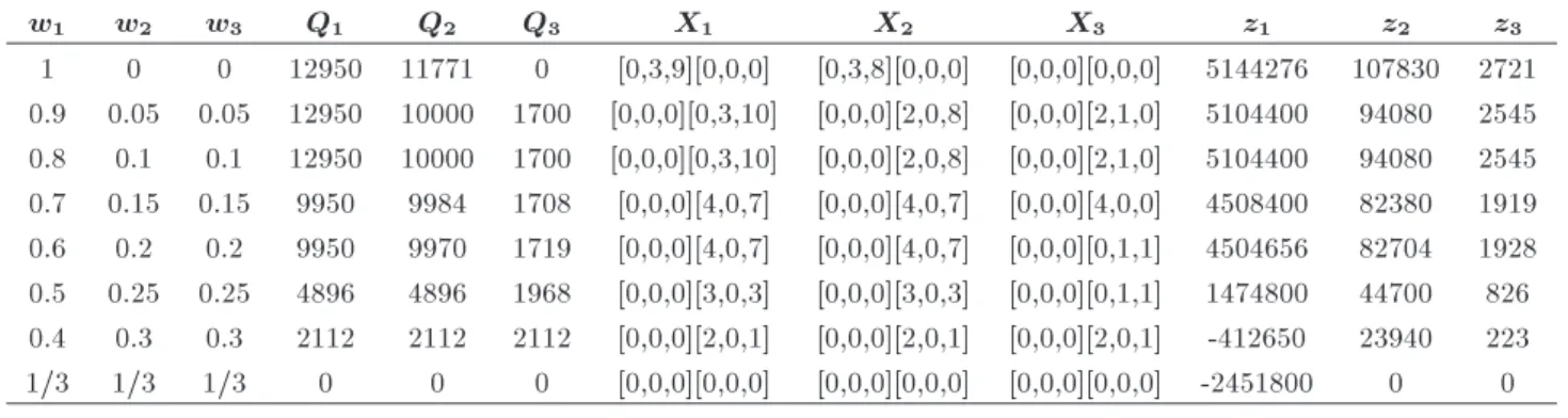
w1 w2 w3 Q1 Q2 Q3 X1 X2 X3 Z1 Z2 Z3
1 0 0 12950 11771 0 [0,3,9][0,0,0] [0,3,8][0,0,0] [0,0,0][0,0,0] 5144276 107830 2721 0.6 0.2 0.2 9950 9970 1719 [0,0,0][4,0,7] [0,0,0][4,0,7] [0,0,0][0,1,1] 4504656 82704 1925
Table 5. The objective functions' components.
Z1 Z2 Z3
R BC LC HC OC PC DC TC GHG-D GHG-T HT HS
w1=1; w2=w3=0 6560000 0 0 8856 100000 1287600 12293 6975 66115 41715 24 2697 w1=0:6; w2=w3=0:2 6104300 1590 302100 50 150000 1127100 9744.4 9060 54204 28500 30 1898
Note: R: Total revenue; BC: Backorder Cost; LC: Lost-sale Cost; HC: Holding Cost; OC: Ordering Cost; PC: Procurement Cost; DC: Disposal Cost; TC: Expected transportation cost;
GHG-D: GHG emission produced by deterioration; GHG-T: GHG emission produced by transportation; HT: Variations in required labor for transportation; HS: Variations in required labor for supplying product;
(iii) Requirement is equal to supply, which means no shortage or inventory exists at the end of the period.
All computations were run applying the CPLEX algorithm accessed via IBM ILOG CPLEX 12.2 on a PC Core (TM) i5 -2.3 GHz and 4.00 GB RAM under Windows 7 Home Premium.
In Table 4, the optimal value of the objective function is reported for two cases: i) rst, the model is solved merely by considering the economic aspect, i.e. w1 = 1 and w2 = w3 = 0; ii) then, by changing
the relative weights (w1 = 0:6, w2 = w3 = 0:2), the
optimal values of decision variables are obtained by taking into account economic (Z1), environmental (Z2),
and social (Z3) aspects. The optimal values of the
objective function components are reported in Table 5 for these two cases.
In Table 4, the optimal conguration of the vehi-cles in each period is reported as a symbol consisting of 2 vectors, each one showing the number of vehicles of each type used in each path. For example, when w1 = 1, w2 = w3 = 0, X1 =
0 3 9 0 0 0 denotes that in the rst period, three vehicles of type 2 and nine vehicles of type 3 are used in Path 1 (desert path) while no vehicle is used in Path 2 (green path).
As Table 4 shows, when w1= 1 and w2 = w3 =
0, the highest value for Z
1 is 5,144,300. Whereas
the worst values for GHGs emissions (Z
2) and labor
variations (Z
3) are obtained in this state.
When the Decision Maker (DM) is concerned with environmental and social criteria as much as costs (w1 = 0:6, and w2 = w3 = 0:2), the optimal
values of the objective functions and decision variables are considerably modied. As Table 4 shows, by considering Z2and Z3 in addition to Z1 (an SSC), the
system loses a part of the prot in comparison with a state that only regards the economic objective (an
economic supply chain). According to Table 4, the environmental and social objectives are improved by about 23.3% and 29.25%, respectively, by losing about 12.4% of total prot.
Considering sustainability criteria, optimal in-ventory and transportation policy and transportation paths are changed. As well, when the DM switches from an economic supply chain to a sustainable one, optimal values of order quantities are more homoge-neous through the planning horizon. Some reasons for this event are i) maintaining variations in the required labor as minimum as possible, and ii) reducing GHG emission as well as costs related to the deterioration process. Values of disposal costs and their related GHGs conrm this statement in Table 5.
8. Sensitivity analysis
In this section, a sensitivity analysis is done regarding the weight (importance) of the objective function. For this purpose, the numerical analysis is done in three stages:
i) Just economic and environmental criteria (Z1 and
Z2) are considered;
ii) Just economic and social criteria (Z1 and Z3) are
considered; and
iii) All economic, environmental, and social criteria (Z1, Z2 and Z3) are considered.
In the rst step, we take into account just economic and environmental criteria (a green supply chain). Thus, w3= 0 and w2= 1 w1. The obtained
results are reported in Table 6 and the Pareto solutions are presented in Figure 2.
According to Table 6 and Figure 2, whenever w1 decreases (the weight of GHG criteria (1 w1)
Table 6. Optimal decision variables and objective functions considering economic and environmental criteria, w2= 1 w1.
w1 Q1 Q2 Q3 X1 X2 X3 z1 z2
Lost prot
(%)
GHG reduction
(%) 1 12950 11771 0 [0,3,9][0,0,0] [0,3,8][0,0,0] [0,0,0][0,0,0] 5144276 107830 { { 0.9 12950 11789 0 [0,0,0][4,1,9] [0,0,0][8,0,7] [0,0,0][0,0,0] 5139400 98655 0.1 8.5 0.8 12950 10071 1632 [0,0,0][3,0,10] [0,0,0][9,0,5] [0,0,0][1,0,1] 5104600 93651 0.8 13.1 0.7 12950 10071 1632 [0,0,0][3,0,10] [0,0,0][9,0,5] [0,0,0][1,0,1] 5104600 93651 0.8 13.1 0.6 12864 10000 1632 [0,0,0][10,0,7] [0,0,0][9,0,5] [0, 0,0][1,0,1] 5055400 92760 1.7 14.0 0.5 9792 9984 1632 [0,0,0][6,0,6] [0,0,0][4,0,7] [0,0,0][1,0,1] 4432300 81120 13.8 24.8
0.1-0.4 0 0 0 { { { -2451800 0 { {
Table 7. Optimal decision variables and objective functions considering economic and social criteria, w3= 1 w1.
w1 Q1 Q2 Q3 X1 X2 X3 z1 z2 Lost
prot (%)
Reductionin labor variations (%) 1 12950 11771 0 [0,3,9][0,0,0] [0,3,8][0,0,0] [0,0,0][0,0,0] 5144276 2721 | | 0.9 12950 10000 1700 [0,3,9][0,0,0] [0,1,8][0,0,0] [0,1,8][0,0,0] 5106600 2535 0.7 6.8 0.8 9950 10000 9587 [0,3,9][0,0,0] [0,3,9][0,0,0] [0,3,9][0,0,0] 4626400 1667 10.1 38.7 0.7 9950 9990 9568 [0,1,8][0,0,0] [0,1,8][0,0,0] [0,1,8][0,0,0] 4036100 1050 21.5 61.4 0.6 9950 9990 9568 [0,1,8][0,0,0] [0,1,8][0,0,0] [0,1,8][0,0,0] 4036100 1050 21.5 61.4 0.5 9950 9950 9534 [0,1,8][0,0,0] [0,1,8][0,0,0] [0,1,8][0,0,0] 4025900 1046 21.7 61.6 0.4 9950 9950 9534 [0,1,8][0,0,0] [0,1,8][0,0,0] [0,1,8][0,0,0] 4025900 1046 21.7 61.6 0.3 2121 2121 2120 [0,0,2][0,0,0] [0,0,2][0,0,0] [0,0,2][0,0,0] -400810 0223 147.7 91.8
0.1-0.2 0 0 0 | | | -2451800 0 | |
Figure 2. Optimal total prot against the optimal GHG emissions.
increase. In this way, when the importance factor (weight) of the green criteria is more than 0.5, purchas-ing is not sound and the supply chain has to be brought to a close. However, in some cases, an acceptable reduction in GHGs emissions is reachable with just a minor reduction in total prot. For example, when w1= 0:7 and w2= 0:3, about 13% GHG reduction can
be obtained with less than 1% reduction in total prot. Besides, as Table 6 shows, when DM is concerned with the environmental criterion, the \green path" is the preferable one even though it is longer and more costly than the other path.
Table 7 presents optimal policies with attention to the economic and social criteria and disregarding the environmental aspect. Thus, w2= 0 and w3= 1 w1.
Here, green criteria are not concerned (w2 = 0). In
all cases, Path 1 (desert path) is therefore the optimal path because it is shorter and more cost-eective.
Moreover, in some periods, an extra cost may be incurred for holding extra equipment whenever varia-tions of required labors are important. For example, when w1= 0:9 (w3= 0:1), the optimal values of order
quantities are determined as Q1= 12950, Q2= 10000,
and Q3 = 1700. However, at Q3 = 1700, the optimal
transportation vehicles are more than the required ones in the third period (a type-2 vehicle (capacity: 900) and eight type-3 vehicles (capacity: 1200)). In fact, to make variations of labors as low as possible, the supply chain is forced to have extra transportation vehicles in period 3, considering required labors in the rst and second periods.
In addition, since the capacity of vehicle type-3 is more than the others, the system prefers to use vehicle type-3 more as the weight of Z3 increases.
In fact, by having high-capacity vehicles, the number of required vehicles for transferring order quantities
Table 8. Optimal decision variables and objective functions with economic, environmental, and social criteria.
w1 w2 w3 Q1 Q2 Q3 X1 X2 X3 z1 z2 z3
1 0 0 12950 11771 0 [0,3,9][0,0,0] [0,3,8][0,0,0] [0,0,0][0,0,0] 5144276 107830 2721 0.9 0.05 0.05 12950 10000 1700 [0,0,0][0,3,10] [0,0,0][2,0,8] [0,0,0][2,1,0] 5104400 94080 2545 0.8 0.1 0.1 12950 10000 1700 [0,0,0][0,3,10] [0,0,0][2,0,8] [0,0,0][2,1,0] 5104400 94080 2545 0.7 0.15 0.15 9950 9984 1708 [0,0,0][4,0,7] [0,0,0][4,0,7] [0,0,0][4,0,0] 4508400 82380 1919 0.6 0.2 0.2 9950 9970 1719 [0,0,0][4,0,7] [0,0,0][4,0,7] [0,0,0][0,1,1] 4504656 82704 1928 0.5 0.25 0.25 4896 4896 1968 [0,0,0][3,0,3] [0,0,0][3,0,3] [0,0,0][0,1,1] 1474800 44700 826 0.4 0.3 0.3 2112 2112 2112 [0,0,0][2,0,1] [0,0,0][2,0,1] [0,0,0][2,0,1] -412650 23940 223 1/3 1/3 1/3 0 0 0 [0,0,0][0,0,0] [0,0,0][0,0,0] [0,0,0][0,0,0] -2451800 0 0
Figure 3. Optimal total prot against the optimal labor variations.
in dierent periods with various values will decrease. In other words, a high-capacity vehicle is able to transfer high and low quantities in dierent periods. Consequently, variations of the required labor for trans-portation will decrease through the planning horizon. Pareto solutions regarding Z1 and Z3 are presented in
Figure 3.
Finally, Table 8 shows the optimal values of decision variables by considering all three objective functions. As this table shows, if DMs put very high values to social and environmental criteria, the supply chain loses its protability. However, managers can play a positive role in improving social and environ-mental indices with just a minor cost (or lost prot).
For example, if the managers set w1 = 0:9,
w2= 0:05, and w3= 0:05, with less than 1% reduction
in total prot, 12.8% and 6.5% improvements will be obtained regarding environmental and social criteria, respectively. This lost prot will be compensated in the medium- and long-term horizons by higher satisfaction, motivation, and, consequently, eciency of workers. In other words, when the workers' sense of belonging and loyalty to their work rise (w3 increases), their
creativity and eciency consequently improve. Finally, with fewer employees and, thus, fewer costs, goals and mission of the organization can be accomplished.
9. Conclusion
Deterioration of products is a major concern in SCM, since most products decrease in quality or value during
their life cycle. Deterioration is a non-linear func-tion made up of many factors such as transportafunc-tion types. The distinct feature of this research is that it is based on numerous characteristics of real de-teriorating products and simultaneously considers all 3 sustainability dimensions in deteriorating products SCM.
This paper considered a centralized forward sup-ply chain for a deteriorating product with various transportation options. Some variables such as the end-customer demand, the partial backordered ratio, and the deterioration rate were assumed to be un-certain. The two sources of deterioration were as-sumed to be: i) deterioration of in-stock inventories, and ii) deterioration of in-transit products, inuenced by both transportation vehicles and transportation paths/modes. The vehicle types (or paths) had a considerable inuence on transportation cost of each product, amount of GHG emission, and deterioration rate of product. A possibilistic mathematical model was developed to determine the optimal replenishment policy, transportation routes, and type of vehicles. It was solved after linearization of various expressions and constraints. The nal solutions were illustrated using a fresh produce center in Tehran, Iran. The results show that DMs can manage green and social issues with a minor reduction in prots. Thus, man-agers may use what-if simulation to see the eects of higher economic and social values of their protabil-ity.
The proposed model is certainly not inclusive and nal, and further research is needed in the following respects:
i) Considering dependency of path and vehicles to the lead-time;
ii) Considering the accident risk related to features of vehicles and paths;
iii) Expanding the proposed model by considering more detailed reverse logistic processes; and
iv) Including multiple suppliers and multiple prod-ucts.
Acknowledgment
This work was supported by Iran National Science Foundation.
References
1. Sepehri, M. \Cost and inventory benets of coopera-tion in multi-period and multi-product supply", Sci. Iran., 18(3), pp. 731-741 (2011).
2. Mirzapour Al-e-hashem, S.M.J., Baboli, A. and Saz-var, Z. \A stochastic aggregate production planning model in a green supply chain: Considering exible lead times, nonlinear purchase and shortage cost func-tions", Eur. J. Oper. Res., 230(1), pp. 26-41 (2013).
3. Devika, K., Jafarian, A. and Nourbakhsh, V. \De-signing a sustainable closed-loop supply chain network based on triple bottom line approach: A comparison of metaheuristics hybridization techniques", Eur. J. Oper. Res., 235(3), pp. 594-615 (2014).
4. Moretti, S., Zeynep Alparslan Gok, S., Branzei, R. and Tijs, S. \Connection situations under uncertainty and cost monotonic solutions", Comput. Oper. Res., 38(11), pp. 1638-1645 (2011).
5. Pishvaee, M.S. and Torabi, S.A. \A possibilistic programming approach for closed-loop supply chain network design under uncertainty", Fuzzy Sets Syst., 161(20), pp. 2668-2683 (2010).
6. Sazvar, Z., Mirzapour Al-e-hashem, S.M.J., Baboli, A. and Akbari Jokar, M.R. \A bi-objective stochastic pro-gramming model for a centralized green supply chain with deteriorating products", Int. J. Prod. Econ., 150, pp. 140-154 (2014).
7. Tsao, Y.-C. \Replenishment policies considering trade credit and logistics risk", Sci. Iran., 18(3), pp. 753-758 (2011).
8. World Commission on Environment and Development, Our Common Future, Oxford University Press, Ox-ford, UK (1987).
9. Wood, D.J. \Corporate social performance revisited", Acad. Manage. Rev., 16(4), pp. 691-718 (1991).
10. Ahi, P. and Searcy, C. \Assessing sustainability in the supply chain: A triple bottom line approach", Appl. Math. Model., 39(10-11), pp. 2882-2896 (2015).
11. Morali, O. and Searcy, C. \A review of sustainable supply chain management practices in Canada", J. Bus. Ethics, 117(3), pp. 635-658 (2012).
12. Seuring, S. \A review of modeling approaches for sustainable supply chain management", Decis. Support Syst., 54(4), pp. 1513-1520 (2013).
13. Brandenburg, M., Govindan, K., Sarkis, J. and Seur-ing, S. \Quantitative models for sustainable supply chain management: Developments and directions", Eur. J. Oper. Res., 233(2), pp. 299-312 (2014).
14. Ramezani, M., Bashiri, M. and Tavakkoli-Moghad-dam, R. \A new multi-objective stochastic model
for a forward/reverse logistic network design with responsiveness and quality level", Appl. Math. Model., 37(1), pp. 328-344 (2013).
15. Das, K. and Rao Posinasetti, N. \Addressing environ-mental concerns in closed loop supply chain design and planning", Int. J. Prod. Econ., 163, pp. 34-47 (2015).
16. Ghare, P.M. and Schrader., G.F. \A model for expo-nentially decaying inventory", J. Ind. Eng., 14(5), pp. 238-243 (1963).
17. Goyal, S.K. and Giri, B.C. \Recent trends in modeling of deteriorating inventory", Eur. J. Oper. Res., 134(1), pp. 1-16 ( 2001).
18. Amorim, P., Gunther, H.-O. and Almada-Lobo, B. \Multi-objective integrated production and distribu-tion planning of perishable products", Int. J. Prod. Econ., 138(1), pp. 89-101 (2012).
19. Prastacos, G.P. \Blood inventory management: an overview of theory and practice", Manag. Sci., 30(7), pp. 777-800 (1984).
20. Validi, S., Bhattacharya, A. and Byrne, P.J. \A case analysis of a sustainable food supply chain distribution system-A multi-objective approach", Int. J. Prod. Econ., 152, pp. 71-87 (2014).
21. Pishvaee, M.S., Razmi, J. and Torabi, S.A. \Robust possibilistic programming for socially responsible sup-ply chain network design: A new approach", Fuzzy Sets Syst., 206, pp. 1-20 (2012).
22. Wang, F., Lai, X. and Shi, N. \A multi-objective optimization for green supply chain network design", Decis. Support Syst., 51(2), pp. 262-269 (2011).
23. El-Sayed, M., Aa, N. and El-Kharbotly, A. \A stochastic model for forward-reverse logistics network design under risk", Comput. Ind. Eng., 58(3), pp. 423-431 (2010).
24. Jamshidi, R., Fatemi Ghomi, S.M.T. and Karimi, B. \Multi-objective green supply chain optimization with a new hybrid memetic algorithm using the Taguchi method", Sci. Iran., 19(6), pp. 1876-1886 (2012).
25. Bakker, M., Riezebos, J. and Teunter, R.H. \Review of inventory systems with deterioration since 2001", Eur. J. Oper. Res., 221(2), pp. 275-284 (2012).
26. Kim, T., Glock, C.H. and Kwon, Y. \A closed loop supply chain for deteriorating products under stochastic container returntimes", Omega, 43, pp. 30-40 (2014).
27. Misra, S.K., Huang, C.L. and Ott, S.L. \Consumer willingness to pay for pesticide-free fresh produce", West. J. Agric. Econ., 16(2), pp. 218-227 (1991).
28. Fearne, A. and Hughes, D. \Success factors in the fresh produce supply chain: insights from the UK", Supply Chain Manag. Int. J., 4(3), pp. 120-131 (1999).
29. Blackburn, J. and Scudder, G. \Supply chain strategies for perishable products: The case of fresh produce", Prod. Oper. Manag., 18(2), pp. 129-137 (2009).
30. Ferguson, M., Jayaraman, V. and Souza, G.C. \Note: An application of the EOQ model with nonlinear holding cost to inventory management of perishables", Eur. J. Oper. Res., 180(1), pp. 485-490 (2007).
31. Shukla, M. and Jharkharia, S. \Agri-fresh produce supply chain management: a state-of-the-art literature review", Int. J. Oper. Prod. Manag., 33(2), pp. 114-158 (2013).
32. Sazvar, Z., Baboli, A. and Jokar, M.R.A. \A replen-ishment policy for perishable products with non-linear holding cost under stochastic supply lead time", Int. J. Adv. Manuf. Technol., 64(5-8), pp. 1087-1098 (2012).
33. Wang, K.-J., Lin, Y.S. and Yu, J.C.P. \Optimizing inventory policy for products with time-sensitive dete-riorating rates in a multi-echelon supply chain", Int. J. Prod. Econ., 130(1), pp. 66-76 (2011).
34. Wee, H.M., Lee, M.-C., Yu, J.C.P. and Wang, C.E. \Optimal replenishment policy for a deteriorating green product: Life cycle costing analysis", Int. J. Prod. Econ., 133, pp. 603-611 (2011).
35. He, Y., Wang, S.-Y. and Lai, K.K. \An optimal production-inventory model for deteriorating items with multiple-market demand", Eur. J. Oper. Res., 203(3), pp. 593-600 (2010).
36. Wee, H.-M. and Chung, C.-J. \Optimising replenish-ment policy for an integrated production inventory de-teriorating model considering green component-value design and remanufacturing", Int. J. Prod. Res., 47(5), pp. 1343-1368 (2009).
37. Liao, J.-J. \An EOQ model with noninstantaneous receipt and exponentially deteriorating items under two-level trade credit", Int. J. Prod. Econ., 113(2), pp. 852-861 (2008).
38. Urban, T.L. \An extension of inventory models with discretely variable holding costs", Int. J. Prod. Econ., 114(1), pp. 399-403 (2008).
39. Dye, C.-Y. \Joint pricing and ordering policy for a deteriorating inventory with partial backlogging", Omega, 35(2), pp. 184-189 (2007).
40. Mahata, G.C. and Goswami, A. \An EOQ model for deteriorating items under trade credit nancing in the fuzzy sense", Prod. Plan. Control, 18(8), pp. 681-692 (2007).
41. Dye, C.-Y. and Ouyang, L.-Y. \An EOQ model for per-ishable items under stock-dependent selling rate and
time-dependent partial backlogging", Eur. J. Oper. Res., 163(3), pp. 776-783 (2005).
42. Luo, W. \An integrated inventory system for perish-able goods with backordering", Comput. Ind. Eng., 34(3), pp. 685-693 (1998).
43. Weiss, H.J. \Economic order quantity models with nonlinear holding costs", Eur. J. Oper. Res., 9(1), pp. 56-60 (1982).
44. Jimenez, M., Arenas, M., Bilbao, A. and Rodrguez, M.V. \Linear programming with fuzzy parameters: an interactive method resolution", Eur. J. Oper. Res., 177, pp. 1599-1609 (2007).
45. Selim, H. and Ozkarahan, I. \A supply chain distribu-tion network design model: an interactive fuzzy goal programming-based solution approach", Int. J. Adv. Manuf. Technol., 36, pp. 401-418 (2008).
Biographies
Mehran Sepehri is Associate Professor of Manage-ment and Economics at Sharif University of Tech-nology, with current research interests in operations management, supply chain, and logistics. He received a PhD in Industrial Engineering and Engineering Management from Stanford University, with previous graduate work at MIT, and a BS degree in Industrial Engineering from Sharif University of Technology. He has 30 years of academic and industrial experience, in USA and Iran, in areas of project management, supply chain management, operation planning, and information systems.
Zeinab Sazvar is Assistant Professor at School of Industrial Engineering at Tehran University. She was a Post-Doc researcher in Graduate School of Management and Economics at Sharif University of Technology. She received her BSc and MSc degrees in Industrial Engineering from Sharif University of Tech-nology (SUT), Iran, in 2006 and 2008, respectively. She is currently a PhD student in Industrial Engineering at SUT, Iran, and in Informatics and Mathematics at INSA Lyon, National Institute of Applied Sciences, France. Her current research interests include supply chain management, inventory control, revenue manage-ment, and operation research.