Research Note
Optimizing a Joint Economic Lot Sizing
Problem with Price-Sensitive Demand
M.R. Akbari Jokar
1;and M. Sheikh Sajadieh
1Abstract. This paper considers the problem of a vendor-buyer integrated production-inventory model. The vendor manufactures the item at a nite rate and delivers the nal goods at a lot-for-lot shipment policy to the buyer. We relax the assumption of uniform demand in the hitherto existing joint economic lot sizing models and analyze the problem where the end customer demand is price-sensitive. The relation between demand and price is considered to be linear. The model proposed, based on the integrated expected total relevant prots of both buyer and vendor, nds out the optimal values of order quantity and mark-up percentage, using an analytical approach. Some numerical examples are also used to analyze the eect of the price-sensitivity of demand on the improvements in joint total prot over individually derived policies. Keywords: Joint economic lot sizing; Mark-up pricing policy; Price-sensitive demand.
INTRODUCTION
In the cases where no coordination exists between supply chain members, the vendor and the buyer will act independently to maximize their own prot. This independent decision behavior usually cannot assure that the two parties, as a whole, reach the optimal state. In traditional inventory management, the opti-mal inventory and shipment policies for manufacturer and buyer in a two-echelon supply chain are managed independently. As a result, the optimal lot size for the purchaser may not result in an optimal policy for the vendor and vice versa. To overcome this diculty, the integrated vendor-buyer model is developed, where the joint total relevant cost for the purchaser as well as the vendor is minimized. Consequently, determining the optimal policies, based on integrated total cost function rather than buyer or supplier individual cost function, results in a reduction of the total inventory cost of the system.
The integrated vendor-buyer problem is called the Joint Economic Lot Sizing (JELS) problem and can be considered as the building block for wider supply chain systems. The global supply chain can be very complex
1. Department of Industrial Engineering, Sharif University of Technology, Tehran, P.O. Box 11155-8639, Iran.
*. Corresponding author. E-mail: [email protected] Received 4 May 2008; accepted 28 April 2009
and link-by-link understanding of joint policies can be very useful.
Goyal [1] was the rst who introduced the idea of a joint total cost for a vendor and a single-buyer scenario, under the assumption of having an innite production rate for the vendor and a lot for lot policy for the shipments from the vendor to the buyer. Banerjee [2] relaxed the innite production rate assumption. Then, Goyal [3] contributed to the eorts of generalizing the problem by relaxing the assumption of lot for lot. He assumed that the production lot is shipped in a number of equal-size shipments. Later, Goyal [4] developed a model where the shipment size increases by a factor equal to the ratio of production rate to demand rate. He formulated the problem and developed an optimal expression for the rst shipment size as a function of the number of shipments. Hill [5] generalized the model of Goyal [4] by taking the geometric growth factor as a decision variable. He suggested a solution method based on an exhaustive search for both the growth factor and the number of shipments in certain ranges. Later, Hill [6] relaxed the assumptions of the shipment policy and developed an optimal solution of the problem. He showed that the structure of the optimal policy includes shipments increasing in size, according to a geometric series, followed by equal-sized shipments.
Joint economic lot sizing models have been ex-tended in many dierent directions. It is beyond
the scope of this paper to discuss all works in detail here. Broadly speaking, the existing literature on JELS may be divided into dierent categories such as quality (e.g. [7]), controllable lead-time (e.g. [8]), setup and order cost reduction (e.g. [9]) and transportation (e.g. [10]). Readers are referred to [11] for a compre-hensive review of the JELS problems.
Despite the large amount of research extending dierent dimensions of JELS problems, most of them are limited to deterministic conditions in which none of the parameters are dependent on each other. However, in practice, there may be some negative or positive coordination between dierent parameters (e.g. price-sensitive demand, time-dependent demand, stock-dependent demand, lot-size stock-dependent lead-times, etc). In this paper, we develop an integrated production-inventory system consisting of a single vendor and single buyer, where the lot from the vendor is trans-ferred to the buyer in a lot-for-lot shipment policy. Unlike previous work in the literature, the demand is considered to be price-sensitive. Here, we analyze how the coordination between two supply chain members will be aected when the end customer demand is price-sensitive.
The paper is organized as follows. In the following section, the notations and assumptions of the problem are introduced. Then, a discussion on independent policies for buyer and vendor as well as on the inte-grated model is given and the optimal value of decision variables is also obtained. Later, some numerical ex-amples and sensitivity analyses are presented. Finally, the paper ndings and directions for future research are summarized.
ASSUMPTIONS
The assumptions of the model are summarized as follows:
1. The integrated system of vendor and single-buyer for a single product is considered.
2. The buyer faces a linear demand as a function of the selling price.
3. Selling price is set based on the unit purchasing price plus a constant percentage mark-up.
4. A nite production rate for the vendor is consid-ered, which is greater than the demand rate. 5. The buyer orders a lot of size Q, when the on-hand
inventory reaches the reorder point.
6. The inventory holding cost for the buyer is more than that for the vendor, i.e. hb> hv.
7. Shipments from the vendor to the buyer use a lot-for-lot policy.
8. Shortage is not allowed.
MATHEMATICAL MODELING
The optimal order quantity and prot margin of the integrated system is derived in this section. We rst obtain the optimal policies if each supply chain member tries to maximize its benet. Then, the policies and prots are compared with the case of an integrated system when they cooperate with each other. We assume that the buyer faces a linear demand, D() = a b(a > b > 0), as a function of his/her unit retail price, which increases as the price decreases. Moreover, we employ a mark-up pricing policy where the selling price is set based on the unit purchasing prices, c, plus a constant percentage mark-up, i.e. = (1 + )c.
Since D() = a bc bc > 0, the maximum percentage mark-up is a=bc 1. The buyer's yearly prot is equal to the gross revenue minus the sum of the purchasing cost, the order processing cost, and inventory holding cost. The buyer wishes to maximize his/her yearly prot function, T BP , through the optimal percentage mark-up, , and order quantity Q, i.e.:
T BP (; Q) = c(a bc bc) (a bc bc)AQ b
hbQ
2 : (1)
For the buyer's percentage mark-up, , which in turn determines the annual demand, D(), the buyer's optimal order size is Q = p2(a bc bc)A
b=hb.
Substituting the optimal order quantity into Equa-tion 1 and simplifying, we obtain:
T BP ()=c(a bc bc) p2(a bc bc)Abhb:
Using the approximation used by Qin et al. [12], the above expression can be rewritten as:
T BP () = c(a bc bc) p2Abhba
[d0(1 + )2c2+ d1(1 + )c + d2];
where d0 = ( 8 + 4p2)(b=a)2, d1 = (12 7p2)(b=a)
and d2= 3p2 4.
Substituting c = (1+) 1and taking the second
derivation of T BP with respect to , we obtain: @2T BP
@2 = 2b 2
p
2Abhbad0:
The above expression is negative if a3> 11A
bhbb2. In
practice, a is usually very large (see [12]) and, thus, the buyer's prot function is concave in , and its optimal value is uniquely determined by equating the rst derivation of T BP to zero.
@T BP
@ = a 2b + bc p
Solving @T BP=@ = 0 and substituting = c(1 + ), the optimal percentage mark-up can be obtained as follows:
=a bc
p
2Abhba[d1+ 2cd0]
2bc + 2cp2Abhbad0 : (2)
Thus, the optimal order quantity can be obtained as:
Q=b(a bc)Ab+p2AbhbaAb(2ad0+ bd1)
hb(b +p2Abhbad0)
1 2
: (3) If there is no cooperation between supply chain mem-bers, then the optimal values of order quantity and mark-up percentage are adopted just based on the buyer prot function. Thus, the orders are received by the vendor at known intervals, T (Figure 1). Therefore, the vendor's yearly prot function is as follows:
T V P = (a bc bc)
c AQv h2PvQ
:
Considering the case in which the buyer (purchaser) is free to choose his/her own pricing and ordering policies, (; Q), then it is straightforward that the individually derived total system prot, T IP (; Q), is equal to the summation of sub-optimal buyer and vendor prots, i.e. T IP (; Q) = T BP + T V P .
Suppose that both parties decide to cooperate and agree to follow the jointly optimal integrated policy. Therefore, the total system prot is going to be maximized, i.e.:
T SP (; Q) = (1 + )c(a bc bc) (a bc bc)(Ab+ Av)
Q Q
2[hb+ hv(a bc bc)=P ]: (4) It can easily be shown that the total system prot is concave in Q for the known values of the buyer
Figure 1. Inventory level against time for buyer and vendor.
percentage mark-up, . Therefore, the optimal order quantity can be obtained as:
Q=
2(a bc bc)(Ab+ Av)
hb+ hv(a bc bc)=P
1 2
: (5)
Substituting the optimal order size into Equation 4 and simplifying, we obtain:
T SP () = (1 + )c(a bc bc) p
2(a bc bc)(Ab+Av)[hb+hv(a bc bc)=P ]:
Using the same approach employed to optimize the buyer prot, the above expression can be rewritten as:
T SP () = (1 + )c(a bc bc) p
2(Ab+ Av)[hb+ hv(a bc bc)=P ]a
[d0(1 + )2c2+ d1(1 + )c + d2]:
Substituting c = (1 + ) 1 and taking the second
derivation of T SP , with respect to , we obtain: @2T SP
@2 = 2b
2p2(Ab+Av)[hb+hv(a bc bc)=P ]ad0:
The above expression is negative and, thus, the total system prot function is concave in and its optimal value is uniquely determined by equating the rst derivation of T SP to zero.
@T SP
@ = a 2b + bc p
2(Ab+ Av)[hb+ hv(a bc bc)=P ]a
(2d0 + d1):
By solving @T SP=@ = 0 and substituting = c(1 + ), the optimal percentage mark-up under the vendor-buyer coordination can be obtained as follows:
=
a bc p2(Ab+Av)[hb+hv(a bc bc)=P ]a[d1+2cd0]
2bc + 2cp2(Ab+ Av)[hb+ hv(a bc bc)=P ]ad0 : (6)
Thus, the optimal order quantity can be obtained as:
Q=pA b+ Av
b(a bc) + !(2ad0+ bd1)
hb(b + !d0)
1 2
; (7)
where:
NUMERICAL EXAMPLES
We consider an example with the following data, P = 3200/year, Av = $400/setup, Ab = $25/order, hv =
$4/unit/year, hb = $5/unit/year, a = 1500, b = 10,
and c = $60/unit.
The optimal values of and Q and the total system prot of the individually optimized model are 0.75, 66.9 and 44106.5, respectively. The corresponding values for jointly optimized model are 0.26, 326.3 and 54310.1. The improvement in joint total prot over individually derived policies is 23.13%, which should be shared in some equitable manner through the mechanism of a side payment to the buyer from the vendor, or a price discount scheme in order to entice the buyer to change his/her lot size and selling price.
In order to gain insight into the eect of some factors such as the price-sensitivity of demand, holding costs and ordering costs, dierent sets of parameter specications have been considered:
1. Four levels for a : a 2 [1300; 1500; 1700; 1900].
2. Six levels for b : b 2 [1; 3; ; 11].
3. Seven levels for buyer holding cost: hb 2
[1; 5; 10; 20; 30; 40; 50].
4. Three levels for buyer ordering cost: Ab 2
[12:5; 25; 50].
5. Seven levels for proportion of vendor setup cost to buyer ordering cost: Av=Ab2 [1; 2; 4; 8; 12; 16; 20].
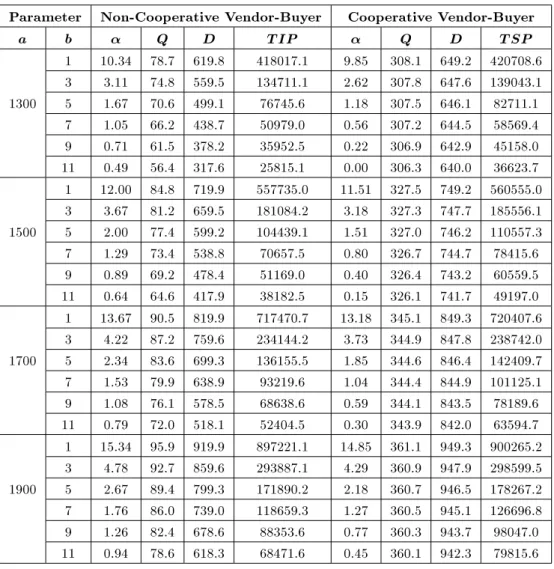
To represent improvements in joint total prot over individually derived policies, we dene the per-centage improvement, P I, as (T SP T IP )=T IP 100. Looking at the results in Table 1, we see that the optimal mark-up percentage is higher in supply chains in which each party tries to maximize his own benet (non-cooperative), compared with the case of a joint system when they cooperate. Since then, the selling prices to end customers will be higher in a non-cooperative situation. Therefore, based on the negative relation between selling price and demand, the incoming demand is less than that in a cooperative situation. As can be seen in Table 1, the demand is
Table 1. Cooperative optimization vs. non-cooperative optimization. Parameter Non-Cooperative Vendor-Buyer Cooperative Vendor-Buyer
a b Q D T IP Q D T SP
1 10.34 78.7 619.8 418017.1 9.85 308.1 649.2 420708.6 3 3.11 74.8 559.5 134711.1 2.62 307.8 647.6 139043.1 1300 5 1.67 70.6 499.1 76745.6 1.18 307.5 646.1 82711.1
7 1.05 66.2 438.7 50979.0 0.56 307.2 644.5 58569.4 9 0.71 61.5 378.2 35952.5 0.22 306.9 642.9 45158.0 11 0.49 56.4 317.6 25815.1 0.00 306.3 640.0 36623.7 1 12.00 84.8 719.9 557735.0 11.51 327.5 749.2 560555.0 3 3.67 81.2 659.5 181084.2 3.18 327.3 747.7 185556.1 1500 5 2.00 77.4 599.2 104439.1 1.51 327.0 746.2 110557.3 7 1.29 73.4 538.8 70657.5 0.80 326.7 744.7 78415.6 9 0.89 69.2 478.4 51169.0 0.40 326.4 743.2 60559.5 11 0.64 64.6 417.9 38182.5 0.15 326.1 741.7 49197.0 1 13.67 90.5 819.9 717470.7 13.18 345.1 849.3 720407.6 3 4.22 87.2 759.6 234144.2 3.73 344.9 847.8 238742.0 1700 5 2.34 83.6 699.3 136155.5 1.85 344.6 846.4 142409.7 7 1.53 79.9 638.9 93219.6 1.04 344.4 844.9 101125.1 9 1.08 76.1 578.5 68638.6 0.59 344.1 843.5 78189.6 11 0.79 72.0 518.1 52404.5 0.30 343.9 842.0 63594.7 1 15.34 95.9 919.9 897221.1 14.85 361.1 949.3 900265.2 3 4.78 92.7 859.6 293887.1 4.29 360.9 947.9 298599.5 1900 5 2.67 89.4 799.3 171890.2 2.18 360.7 946.5 178267.2 7 1.76 86.0 739.0 118659.3 1.27 360.5 945.1 126696.8 9 1.26 82.4 678.6 88353.6 0.77 360.3 943.7 98047.0 11 0.94 78.6 618.3 68471.6 0.45 360.1 942.3 79815.6
22.69% lower in non-cooperative vendor-buyer supply chains, on average. Additionally, there is not a signicant demand variation in joint optimization as price sensitivity change. However, the demand for individual/non-cooperative optimization shows a 40% reduction, as moving from b = 1 to b = 11, on average.
Some other facts can also be discerned from Table 1. The optimal order quantity is considerably higher in joint optimization versus individual optimiza-tion. The main reason is that since the setup cost of the vendor is higher than the ordering cost of the buyer, the model enlarges the order quantity to lessen the number of ordering and setups. Based on the results shown in Table 1, the order quantity of the cooperative model is almost 4.3 times bigger than that in the non-cooperative model.
Moreover, Table 1 shows that as the price-sensitivity of demand, b, increases, mark-up percent-ages decrease in both joint and individual optimiza-tions. That is because the models try to condense the eect of selling prices and control the demand reductions.
Figure 2 shows the percentage improvement in joint total prot over individually derived policies for a range of a and b. As can be seen in Figure 2, P I increases for cases where demand is more price-sensitive. This result conrms that it will be more benecial for the buyer and vendor to cooperate with each other in competitive environments where end customers have a number of purchasing choices and can easily shift to other less expensive supply chains.
Furthermore, the increase in the total system prot shows an exponential behavior where the change in P I is 1.84%, moving from b = 1 to b = 3, while this value is equal to 9.95%, moving from b = 9 to b = 11, on average.
We also endeavor to examine whether the buyer
Figure 2. Eect of price-sensitivity on the benets of vendor-buyer coordination.
holding cost has any eect on the benets of vendor-buyer coordination. As can be seen in Figure 3, the improvement percentage, P I, increases by buyer hold-ing costs. However, this increase in the improvement percentage is of a diminishing kind, with most of the saving obtained from an initial increase. The reason is that as buyer holding costs increase, the optimal order quantity in the non-cooperative model decreases as well, much faster than that in the joint model. Thus, the total prot of non-cooperative models reduces and, consequently, cooperation becomes more attractive for supply chain members.
Figure 4 illustrates the eect of the proportion of vendor to buyer ordering cost on P I. As illustrated, the improvement percentage increases by Av=Ab. In
other words, it will be more benecial for supply chains to cooperate with each other, as their ordering and setup costs are far from each other. However, the improvement in P I is negatively aected by buyer ordering cost decreases. For example, P I improvement is 7.8%, moving from Av=Ab= 1 to Av=Ab= 20 (from
19.30% to 27.10) when Ab = 50, but it is 3.65% when
Ab= 12:5.
Figure 3. Eect of buyer's holding cost on P I.
Figure 4. Eect of setup cost to ordering cost proportion on the benets of vendor-buyer coordination.
CONCLUSION AND DIRECTIONS FOR FUTURE RESEARCH
We developed an integrated production-inventory model in which the objective is to maximize the joint total prot of the buyer and the vendor by optimizing the ordering and pricing policies. The developed model is a JELS model, where the lot from the vendor is transferred to the buyer in a lot-for-lot shipment policy. Unlike previous works in the literature, the demand is considered to be price-sensitive. Here, we used an analytical approach to nd the optimal order quantity and mark-up percentage. Moreover, we analyzed how the coordination between two supply chain members will be aected when the end customer demand is price-sensitive.
We also compared the case of a cooperative system, when supply chain members cooperate with each other, over individually derived policies. The numerical example results showed that when demand is more price-sensitive, the system prot achieved by joint optimization is signicantly larger than that obtained by individual optimization. Therefore, when demand is more price-sensitive, the supplier should employ some coordination mechanisms such as volume discount, to achieve higher channel coordination. This result conrms that it will be more benecial for the buyer and vendor to cooperate with each other in competitive environments, where end customers have a number of purchasing choices and can easily shift to other less expensive supply chains, i.e. demand is more price-sensitive.
One of the future research directions is to extend this study for other shipment policies such as non-delayed, equal-sized shipment policies. Developing the model to the multi-supplier case is also proposed for future research. Moreover, in this paper, we considered a linear price-demand relation, however, it might be useful to analyze other demand functions (e.g. log-linear) as well.
NOMENCLATURE
D demand rate as a function of unit selling price
P production rate of the vendor Q buyer's order quantity
c the buyer unit purchasing price the buyer unit selling price mark-up percentage Av vendor's setup cost
Ab buyer's ordering cost
hv inventory holding cost for the vendor
per unit time
hb inventory holding cost for the buyer
per unit time REFERENCES
1. Goyal, S.k. \An integrated inventory model for a single supplier-single customer problem", International Journal of Production Research, 15(1), pp. 107-111 (1976).
2. Banerjee, A. \A joint economic-lot-size model for purchaser and vendor", Decision Science, 17, pp. 292-311 (1986).
3. Goyal, S.K. \A joint economic-lot-size model for pur-chaser and vendor: A comment", Decision Science, 19, pp. 236-241 (1988).
4. Goyal, S.K. \A one-vendor multi-buyer integrated inventory model: A comment", European Journal of Operational Research, 82, pp. 209-210 (1995). 5. Hill, R.M. \The single-vendor single-buyer integrated
production-inventory model with a generalized policy", European Journal of Operational Research, 97, pp. 493-499 (1997).
6. Hill, R.M. \The optimal production and shipment policy for the single-vendor single-buyer integrated production-inventory model", International Journal of Production Research, 37, pp. 2463-2475 (1999). 7. Asco, J.F., Paknejad, M.J. and Nasri, F. \Quality
improvement and setup reduction in the joint economic lot size model", European Journal of Operational Re-search, 142, pp. 497-508 (2002).
8. Hoque, M. and Goyal, S.K. \A heuristic solution procedure for an integrated inventory system under controllable lead-time with equal or unequal sized batch shipments between a vendor and a buyer", International Journal of Production Economics, 102, pp. 217-225 (2006).
9. Chang, H.C., Ouyang, L.Y., Wu, K.S. and Ho, C.H. \Integrated vendor-buyer cooperative inventory models with controllable lead time and ordering cost reduction", European Journal of Operational Research, 170, pp. 481-495 (2006).
10. Ertogral, K., Ben-Daya, M. and Darwish, M. \Produc-tion and shipment lot sizing in vendor-buyer supply chain with transportation cost", European Journal of Operational Research, 176, pp. 1592-1606 (2007). 11. Ben-Daya, M., Darwish, M. and Ertogral, K. \The
joint economic lot sizing problem: review and ex-tensions", European Journal of Operational Research, 185, pp. 726-742 (2008).
12. Qin, Y., Tang, H. and Chonghui, G. \Channel co-ordination and volume discounts with price-sensitive demand", International Journal of Production Eco-nomics, 105, pp. 43-53 (2007).