Simulation of Random Irregular Sea Waves for Numerical and Physical Models Using Digital Filters

Simulation of Random Irregular

Sea Waves for Numerical and

Physical Models Using Digital Filters

M.J. Ketabdari

_{and A. Ranginkaman}

Abstract. Wind waves, which are one of the most important phenomena in the marine environment, are generally progressive in nature and can move far distances out of their area of formation. Thus, an understanding of wave hydrodynamics and their eects is important for engineers in the design and construction of marine structures and coastal management. Signicant insights may be gained from numerical and laboratory studies. Often the waves simulated in numerical and physical models do not have the full characteristics of real sea waves. It is then necessary to present a reliable method of wave simulation for numerical and laboratory wave umes. In this paper, the results of numerically simulated water waves, using digital lters, are presented. A model has been developed to simulate a water wave prole from dierent target spectra using WNDF methods. The results showed that the WNDF method involves good stochastic wave characteristics if a suitable spectrum is used as target. The results have implications for the numerical or laboratory estimation of wave forces on model oshore or coastal structures.

Keywords: Wave spectrum; Digital lter; White noise; Random irregular waves; WNDF method.

INTRODUCTION

To design coastal and oshore structures, it is required to evaluate the eect of sea waves on the structures. To accomplish this, mathematical and physical models are needed. Therefore, the problem has dierent features. On the one hand, the structure should be modeled properly, on the other hand, the exciting force should be simulated. In some model tests, monochromatic waves are used. However, waves in fully developed seas are usually random and irregular and can be expressed by their energy spectrum over a range of frequencies. Hence, ideal sine waves with a single frequency cannot express all features of real sea waves. This may mislead the results. Therefore, methods of generating irregular waves have been developed during the past few decades.

1. Department of Marine Technology, Amirkabir University of Technology, Tehran, P.O. Box 15875-4413, Iran.

*. Corresponding author. E-mail: [email protected] Received 16 April 2007; received in revised form 21 September 2007; accepted 1 December 2007

IRREGULAR WAVE SIMULATION

The technology of wave generation for numerical and physical models has developed rapidly during the past two decades. It has beneted mainly from advances in control system theory and computer hardware. Real wind waves in the eld are highly irregular and seldom exhibit a sinusoidal nature. In the past decades, attempts have been made to generate laboratory waves which closely approximate natural wave trains. Al-though real sea waves are 3D, coastal engineers usually reproduce these natural waves as a 2D process, due to the fact that 2D irregular waves are more amenable to theoretical treatment. Nevertheless, they oer some understanding of the complexities of 3D real sea states. The techniques for synthesizing irregular waves for marine engineering model studies can be categorized as follows:

1. Superposition of a nite number of sine waves; 2. Prototype measurement of wind wave time series; 3. Deterministic irregular wave trains (DSA method);

4. Non-deterministic irregular wave trains (NSA method);

5. Filtering white noise using proper digital lters (WNDF method).

Methods 1 to 4 have been already used for irregular wave generation and dierent researchers have referred to these methods and their advantages and disadvantages [1-5]. The last method, which is wave simulation via the ltering of white noise, has been rarely used in marine engineering due to its complexity. Therefore, in this paper, irregular random wave synthesis by this method is examined.

DIGITAL FILTERING Design Theory

Digital lter is a Single Input-Single Output (SISO) system [6], which is Linear Time Invariant (LTI) and can be shown as in Figure 1.

Considering X1(t) and X2(t) as two arbitrary

inputs and a, b as two arbitrary real constants, this system is called linear if:

L(aX1(t) + bX2(t)) = aL(X1(t)) + bL(x2(t)): (1)

The system is called time invariant, if:

L(X(t t0)) = Y (t t0); (2)

in which t0 is an arbitrary time shifting. A stochastic

process is a rule that represents a function f(t; ) from t and . For a stochastic process, rst order distribution and rst order density are dened as the following [7]:

F (x; t) = pfx(t) xg; (3)

f(x; t) = @F (x; t)_@x ; (4)

in which pfxg is the probability function. The average of a stochastic process for a stochastic variable, x(t), is called the Expected value as follows:

E(x(t)) = Z ₁

1xf(x; t)dx: (5)

The autocorrelation function is dened as: Rx(t1; t2) =

Z ₁

1

Z ₁

1x1x2f(x1; x2; t1; t2)dx1dx2

= Efx1(t)x2(t)g; (6)

Figure 1. A linear single input-output system.

where f is the stochastic variable, x(t1) = x1 and

x(t2) = x2.

A stochastic process, x(t), is called Strict-Sense Stationary (SSS) if it is statistically independent of the distance from the origin. In other words, x(t) is statis-tically equal to x(t + c), where c is an arbitrary value. Also, a stochastic process, x(t), is called Wide-Sense Stationary (WSS) when the expected value (average) is constant: Efx(t)g = and its autocorrelation relates only with a dierence between t1 and t2( = t1 t2)

and is independent of t1 and t2 values:

Efx(t + )x_{(t)g = R(): (7)}

White noise is a noise with a power spectrum that is independent of frequency and its value at any frequency is:

Sw(f) = q = N₂0: (8)

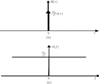
This noise is called white noise because the density spectrum of this process is widely distributed in the frequency domain as white light. The autocorrelation function is the inverse Fourier transform of the power spectrum density. Therefore, the autocorrelation func-tion of white noise can be represented as follows (see Figures 2a and 2b):

Rw() = q() = N₂0(): (9)

Linear Time Invariant System with Stochastic Process Input

For a linear system, L, with input x(t) and output y(t), if x(t) is a stochastic process, then the output, y(t), is also a stochastic process. To nd the relation

Figure 2. a) White noise spectrum and b) Its autocorrelation function [8].

between the output autocorrelation function and the input autocorrelation function, at rst we know that:

EfL[x(t)]g = L[Efx(t)g]: (10) Since system L and function E are both linear, we have: Rxy(t1; t2) = L2[Rxx(t1; t2)]; (11)

where Rxyis cross correlation of x and y and L2means

that the system acts on t1 as a variable and t2 as

a parameter. By this relation, we can develop the relation between input and output spectrums. For x(t) as a WSS process, the power spectrum density is the Fourier transform of its autocorrelation function:

S(!) = Z ₁

1Rxx()e

j!_{d: (12)}

Since R( ) = R_{() and S(!) is a real function of}

variable !, by using the inverse Fourier transform, we have:

Rxx() = ₂1

Z ₁

1S(!)e

j!z_{d!: (13)}

It means that Rxx(z) can be obtained from the

spec-trum, S(!) [9]. We can nd innite processes that have the same spectrum, S(!). Hereby, two methods are explained to gain these processes.

a) Method 1

Consider a random process as follows (see [10]):

x(t) = aej(!t ')_{; (14)}

in which a is a real constant, ! is a stochastic variable with density of f!(!) and ' is an independent

stochastic variable with uniform density on (0, 2). It can be proved that this process is a WSS process with zero mean and the following autocorrelation function:

Rx() = a2Efej!g = a2

Z ₊₁

1 f!(!)e

j!_{d!: (15)}

Therefore, its spectrum can be found as: Sx(!) = F fRx()g;

and:

Rx() =₂1

Z ₊₁

1 Sx(!)e j!_d!;

leading to:

Sx(!) = 2a2f!(!): (16)

This relates the power spectrum density function of x, with the probability density function of !. Substituting = 0 in Equation 16 yields:

Rx(0) = a2

Z ₊₁

1 f!(!)d! = a 2

=₂1 Z ₊₁

1 S!(!)d!: (17)

Thus, to nd the stochastic process of its spectrum, we suppose that the probability density function is:

f!=S(!)_2a2; (18)

so that a2 _{= Rx(0) and R(0) is the signal's power of}

process. In this way, the process of Equation 15 would have the spectrum of S(!).

b) Method 2

The linear time invariant system with impulse response h(t) is shown in Figure 3.

In this system if x(t) is a WSS process, then the relation between output and input autocorrelation would be as follows [11]:

Rxy(t) = h( t)Rxx(t); (19)

Ryy(t) = h(t)Rxy(t): (20)

Leading to:

Ryy(t) = Rxx(t)h(t)h(t): (21)

Taking the Fourier transform from both sides of the above equation, we have:

Syy(f) = Sxx(f)H(f)H(f) = Sxx(f) jH(f)j2: (22)

If the input of the system is white noise with q = 1, then:

Rxx() = q() = ();

Sxx(f) = 1;

Syy(f) = Sxx(f) jH(f)j2) jH(f)j =

q

Syy(f): (23)

Figure 3. A linear time invariant system with impulse response, h(t).

So to achieve a process with a certain spectrum, a system with the following transfer function can be dened:

jH(f)j =pS(f); H(f) = 0: (24) If the input of such a system is white noise, then the output of the system will have the spectrum, S(f):

Syy(f)=jH(f)j2Sxx(f)=(

p

S(f))2_{1=S(f): (25)}

SIMULATION RESULTS

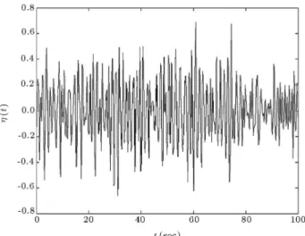
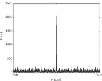
As mentioned in the previous section, if the transfer function of a lter is the root of the spectrum and the input to this lter is white noise, then, the output of the lter would be a random irregular wave that has the same spectrum. So, a lter with a white noise input can be designed, leading to an output which is the desirable simulated wave (random irregular wave). Therefore, based on the above mentioned algorithm, software was developed to generate random irregular waves by white noise ltering. Using three classic target spectra: Pierson Moskowitz, JONSWAP and Bretschneider Spectrum, sample irregular random waves were generated. Figures 4 to 6 show the time histories of the generated wave using dierent target spectra. It can be seen that the results of the simulation are dierent wave time histories, as a random process is used. However, the time histories alone cannot give us further information about these waves. Figures 7 to 9 compare these wave energy spectra with target ones. This can be considered as a criterion for the accuracy of the method. It is clear from these gures that the output spectrum uctuates around target one in all the three classic spectra. Figures 10 to 12 present the autocorrelation of generated waves using dierent target spectra. This can be used as a criterion for evaluating the randomness of the signals. Figures 13 to 15 compare the ideal and output probability density function for the three spectra. It can be seen that the values of 2_{for the Pierson-Moskowitz, JONSWAP and}

Bretschneider target spectra are 0.613, 0.577 and 0.689, respectively.

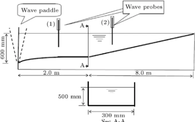
APPLICATION OF WNDF METHOD IN MARINE ENGINEERING

The behavior of numerical and experimental models of coastal and oshore structures is often examined against random irregular waves. The time histories of the irregular waves generated by the WNDF method can be used as an input to these models. Figure 16 schematically shows the experimental apparatus for wave generation and recording in the laboratory ume. The wave tank had a depth of 600 mm, width of

Figure 4. Time histories of generated wave using Pierson-Moskowitz spectrum.

Figure 5. Time histories of generated wave using JONSWAP spectrum.

Figure 6. Time histories of generated wave using Bretschneider spectrum.

Figure 7. Comparison of spectrum of generated wave and target spectrum (Pierson-Moskowitz).

Figure 8. Comparison of spectrum of generated wave and target spectrum (JONSWAP).

Figure 9. Comparison of spectrum of generated wave and target spectrum (Bretschneider spectrum).

Figure 10. Autocorrelation of generated wave using Pierson-Moskowitz spectrum.

Figure 11. Autocorrelation of generated wave using JONSWAP spectrum.

Figure 12. Autocorrelation of generated wave using Bretschneider spectrum.

Figure 13. Pdf of generated wave using Pierson-Moskowitz spectrum.

Figure 14. Pdf of generated wave using JONSWAP spectrum.

Figure 15. Pdf of generated wave using Bretschneider spectrum.

300 mm and length of 10 m. This ume also had a long sloping beach with a slope of approximately 8% to simulate coastal conditions.

An irregular wave was generated using JON-SWAP as the target spectrum (see Figure 17). This wave was fed to the ap type wave paddle of the above mentioned wave ume using a DTA converter. The

Figure 16. Schematic of experimental set-up for wave generation.

Figure 17. Target spectrum and relevant simulated wave by WNDF method as input to wave paddle.

scale of the wave could be adjusted by an amplier. Figure 18a shows the recorded wave at wave probe no 1. It can be seen that the generated wave is not in phase with the input one. It is because the wave probe has a distance from the wave paddle. The calculated power spectrum of this wave can be seen in Figure 18b. It is clear that the output spectrum is dierent from the target one. This is because of the nonlinear interaction of the rigid paddle and water as it moves forward and backward. Figure 19 shows another input signal simulated by another method and recorded by wave probe no. 2. It is evident that in this case the wave is distorted by the shallow water bed eect.

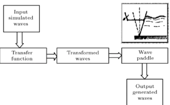
However it is possible to solve this problem using a transfer function. Figure 20 shows the diagram box of the relevant procedure. It should be noted that the transfer function depends on the geometry of the wave ume and the wave generating hardware system. Nonetheless, nding it is not the aim of this piece of work at this stage. Nevertheless, it is possible to overcome these discrepancies between input and output data, nding a proper transfer function.

Figure 18. Recorded wave in the wave ume by probe no. 1 and its calculated spectrum.

Figure 19. Simulated and generated wave in the wave ume recorded by probe no. 2.

Figure 20. Diagram box of ume wave generation using transfer function.

Consequently, having a qualitative irregular signal such as that obtained by the WNDF method, is vital for getting reliable results from physical coastal and oshore models.

CONCLUSIONS

The WNDF method, which is a frequency domain procedure, was employed to simulate random irregular waves for numerical and laboratory models of a marine environment. Three well-known spectral wave ener-gies, known as the Pierson-Moskowitz, JONSWAP and Bretschneider spectra, were used as the target. Choos-ing the square root of the spectrum as the transfer function of a lter and the input to this lter as a white noise, a random irregular wave was generated. The time histories of generated waves using dierent spectra show that apparently random irregular waves are ob-tained as output. The spectrum of the generated wave

shows that it uctuates around the target spectrum. This result is in fact desirable as realistic sea waves demonstrate a non-smooth spectrum. In addition, the spectrum shows that generated waves associated with wave energy in a range of frequencies have the character of irregular sea waves. To be certain about the randomness of waves, the autocorrelation function was used. The results showed that the generated waves are reasonably random. The comparison of the power spectrum density function of output waves with ideal ones also shows an acceptable deviation. One of the most important advantages of this method is the possibility of placing additional constraints on specic wave characteristics such as the number of waves in a wave time series, frequency band, time domain, wave amplitude, wave energy, wave nonlinearity and other favorable characteristics. It is also possible to make the required lters using electronic hardware. Therefore, the WNDF method can be used as a powerful tool for one-sided random irregular wave generation. The re-sults are also promising for generating multi-directional irregular waves for 3D models by expanding this model and using directional wave spectra as input.

REFERENCES

1. Rice, S.O. \Mathematical analysis of random noise", Bell System Tech. J., 23 (1944) and 24 (1945), (Reprinted in selected papers on noise and stochastic processes, N. Wax, Ed., Dover Pub. Inc., N.Y., pp. 123-144 (1954).

2. Gravesen, H. and Sorensen, T. \Stability of rub-ble mound breakwaters", Proc. 23rd PIANC Conf., Leningrad (1977).

3. Funke, E.R. and Mansard, E.P.D. \A rationale for the use of the deterministic approach to laboratory wave generation", Proc. 22nd Cong. Int. Associated for Hydraulic Res., pp. 153-195 (1987).

4. Funke, E.R., Mansard, E.P.D. and Dai, G. \Realizable wave parameters in a laboratory ume", Proc. 21st Int. Conf. Coastal Eng., ASCE, 1, pp. 835-848 (1988). 5. Hughes, S.A., Physical Models and Laboratory

Tech-niques in Coastal Engineering, JBW Printers & Binders Pte. Ltd., London (1993b).

6. Ahmed, N. and Natarajan, T., Discrete-Time Signals and Systems, Reston Pub. Company, Inc., Virginia (1983).

7. Bendat, J.S. and Piersol, A.G., Random Data Analysis and Measurement, John Wiley and Sons Inc., New York (1986).

8. Haykin, S., Communication Systems, John Wiley & Sons Inc., New York (1993).

9. Oppenheim, A.V. and Willsky, A.S., Signals and Systems, 2nd Ed., Edward Arnold Pub. Co., London (1996).

10. Cohen, A. \Biomedical signal processing", Time and Frequency Domain Analysis, I, CRC Press, Inc. (1986). 11. Shanmugan, K.S and Breipohl, A.M., Random Signals-Detection, Estimation and Analysis, John Wiley and Sons, Inc., New York (1998).