A Shortest Path Problem in an
Urban Transportation Network Based
on Driver Perceived Travel Time
H. Ramazani
1, Y. Shafahi
1;and S.E. Seyedabrishami
1Abstract. This paper proposes a method to solve shortest path problems in route choice processes when each link's travel time is a fuzzy number, called the Perceived Travel Time (PTT). The PTT is a subjective travel time perceived by a driver. The algorithm solves the fuzzy shortest path problem (FSPA) for drivers in the presence of uncertainty regarding route travel time. For congested networks, the method is able to nd the shortest path in terms of perceived travel time and degree of saturation (congestion) along routes at the same time. The FSPA can be used to support the fuzzication of trac assignment algorithms. The applicability of the resulting FSPA for the trac assignment was tested in conjunction with incremental trac loading and was applied to a large-scale real network. The results of the trac assignment based on the FSPA, User Equilibrium (UE) and a stochastic loading network model (Dial's assignment algorithm) were compared to the observed volume for certain links in the network. We conclude that the proposed method oers better accuracy than the UE or Dial's assignment algorithm for the network under testing. Keywords: Fuzzy sets; Perceived travel time; Route choice; Shortest path; Urban network.
INTRODUCTION
An important consideration in the route choice pro-cess for urban transportation networks is how drivers perceive link travel time and nd the appropriate path to their destination based on path travel time. Traditional assignment algorithms (e.g. incremental assignment or User Equilibrium (UE)), assume that all drivers experience the same link travel time. In reality, this is not the case, because drivers may have dierent perceptions of travel time for a particular path. Another assumption behind traditional assign-ment algorithms is that each individual uses a single value for travel time. For a more realistic description of the problem, this assumption can be disregarded when one knows that the trac demand and consequently the volume of each link are stochastic in nature or that an unexpected event may inuence a link's travel time. The variation in trac volume in conjunction with
1. Department of Civil Engineering, Sharif University of Tech-nology, Tehran, P.O. Box 11155-9313, Iran.
*. Corresponding author. E-mail: shafahi@sharif.edu
Received 11 November 2009; received in revised form 9 April 2010; accepted 14 June 2010
the degree of saturation and unexpected events may aect the driver's perception of travel time. Generally a driver's perception of link travel time arises from his/her experience in previous route choice scenarios between the same origin and destination.
Many studies have been carried out on travel time uncertainty in route choice. Two dierent meth-ods are applicable to model travelers' choices under uncertainty. One uses a probabilistic choice model that is often based on utility functions. The other method, discussed in this paper, makes use of fuzzy logic. Fuzzy logic is a powerful technique used for considering uncertainties related to human perception in modeling contexts. Here, we establish an innovative fuzzy denition for Perceived Travel Time (PTT) using membership functions and the route choice process. Also, a Fuzzy Shortest Path Algorithm (FSPA) based on a labeling procedure is proposed for application to trac assignments in an urban transportation network in which a PTT is assigned to each link.
A great deal of recent research has attempted to use fuzzy concepts to solve the shortest path problem. The most recent papers addressing the fuzzy shortest path problem include those by Chang and Lee (1999)
who used an overall existence ranking index to assign dierent types of status (optimistic, pessimistic or neutral person) to drivers [1], and Okada and Soper (2000) who introduced an order relation between fuzzy numbers based on the concept of a fuzzy minimum [2]. In another paper, Okada (2004) considered interactiv-ity among fuzzy numbers assigned to arc length by dening a new comparison index [3]. Blue et al. (2002) formulated several standard graph-theoretic problems (shortest path and minimum cut) for fuzzy graphs using a unied approach that is distinguished by its uniform application of guiding principles, such as the construction of membership grades via the ranking of fuzzy numbers etc. [4]. Chuang and Kang (2005) assigned a fuzzy set with a triangular membership func-tion to each arc length and proposed a new algorithm to deal with the fuzzy shortest problem [5]. They also proposed a heuristic procedure to nd the Fuzzy Shortest Path Length (FSPL), among all possible paths in a network, based on the idea that a crisp (non-fuzzy) number is a minimum if, and only if, any other number is larger than or equal to it. They then proposed a way to measure the degree of similarity between the FSPL and each fuzzy path length. The path with the highest degree of similarity was chosen as the shortest path. Moazeni (2006) dened an order relation between fuzzy quantities with nite support [6]. Ji et al. (2007) considered dierent decision criteria to specify the shortest path in a fuzzy environment and to solve the model using hybrid intelligent methods. The hybrid intelligent methods included a combination of simulations and a genetic algorithm [7]. Hernandes et al. (2007) proposed an iterative algorithm that uses a generic ranking index for comparing the fuzzy numbers involved in the problem, in such a way that each time the decision-maker wants to solve a concrete problem, (s)he can choose (or propose) the ranking index that best suits that problem [8].
Some studies have used fuzzy theory in route choice contexts to address behavioral characteristics. The most important studies are by the following au-thors: Teodorovic and Kikuchi who proposed [9] an ap-proximate reasoning model used for trac assignment between two alternative routes on a highway network; Murat and Uludag [10] who compared a fuzzy logic model with a linear regression model to show how the application of fuzzy logic to dening link travel times increases route choice accuracy; and Binetti and De Mitri [11] who used fuzzy numbers to represent the imprecision in path costs for a road network. Additionally, Binetti and De Mitri utilized the method of successive averages to generate user equilibrium ows in a simple network. The model yielded realistic results. Finally, Arslan and Khisty [12] presented a heuristic way of handling fuzzy perceptions and used the Analytical Hierarchy Process (AHP) to explain
route choice behavior in transportation systems. This method provided intuitive and promising results.
In comparison to those mentioned above, the present study demonstrates a fuzzy denition of PTT by developing the route choice process using a shortest path algorithm. The algorithm utilizes a labeling procedure in an urban transportation network with perceived fuzzy travel time. The proposed FSPA is dened in such a way that it can easily be used in fuzzy assignment algorithms. The criterion used in this paper to compare link travel times as fuzzy numbers is more consistent with the actual route choice process.
In the next section, the method of formulating a PTT using fuzzy sets is described. After that, a route choice decision-making process is presented followed by the FSPA. The results for a real network are shown in the subsequent section and the conclusions are presented in the last section.
PTT DEFINITION AND CONCEPTS
Generally, there are two kinds of uncertainty. The rst type of uncertainty is derived from the imprecision that is inherent in taking measurements or surveys, which can be aected by unpredicted events (e.g. an acci-dents or weather conditions) or demand uctuations. The second type is linked with human perception. According to the work of Zadeh [13,14], probability theory is very useful for dealing with the uncertainty inherent in measurements; however, it is not very useful for dealing with the uncertainty associated with human perceptions. The former involves crisp sets, while the latter involves fuzzy sets [15]. Because PTT uncertainty is derived from human perceptions, it is more useful to use fuzzy concepts when considering the uncertainty in drivers' deductions for PTT.
Although many researchers have attempted to determine travel time uncertainty using fuzzy concepts, no distinct process has been applied to fuzzy trac assignment models to build and dene Membership Functions (MF) [16]. In fact, the denition of a MF in existing fuzzy models is not well-constructed. Generally, a triangular MF is used for the PTT to simplify the computation process. The triangular MF has three specication parameters: the MF center, the right limit, and the left limit. The PTT MF center denotes the most common travel time of a link. The right limit is associated with the highest possible travel time. The left limit is associated with the minimum possible travel time. Typically, the computed travel time of a link based on its assigned volume is assumed to be the center of the PTT MF for that link.
To dene the left and right limits of the MFs in this work, a method is proposed that reects the trac state of each link. Basically, this method assumes that the volume of each link varies from day
to day. This variation causes dierences in travel time and consequently users have a set of travel times in mind. The PTT is modeled using fuzzy numbers. The assumption of variable volumes for each link is not unique for this study, as it is also used in probabilistic trac assignment, where link volume is a random variable [17]. The method assumes that the volume of each link varies between a lower and an upper bound that are (1 l) and (1 + r) times the most observed
volume (i.e. the volume assigned to the link within the assignment steps), respectively (l and r are two
numbers specify a lower and upper bound for link volume, respectively). As shown in Figure 1, the PTT is assumed to have a triangular membership function. The left and right limits of the PTT MF correspond to the travel times of the lower and upper bounds of the volume, respectively. As mentioned earlier, the travel time for the most observed volume is the center of the PTT MF. Hence, knowing (l), (r) and the volume
assigned to the link, the PTT MF can be constructed. The PTT triangular membership function parameters, ~t, are the left, center and right limits of the PTT membership function and are denoted as tl, tc, tr,
respectively. Function t[x] calculates the link travel time as a function of the link trac volume shown by x. The specication parameters of the triangular MF (i.e. the left, center and right limits shown in Figure 1) are highly dependent on the problem at hand. These parameters can be calculated by comparing the results of the trac assignment used in the PTT MF, shown in Figure 1, to the volume of the observed links. A computational procedure for the estimation of is suggested in the PTT application section using a real network assignment algorithm. However, a PTT MF can also be determined through use of questionnaires that ask drivers for their PTT for a specic link, but in this paper, no PTT data are available.
The PTT MF for each path is computed using the fuzzy summation of the PTT MFs for all links. One of the advantages of triangular MFs over other types of (non-linear) fuzzy numbers is that there is a closed form for the summation of these numbers. For example, the
Figure 1. PTT MF shape and parameters.
PTT MF for path K is calculated as follows: ~tK =
X
a2K
ta[(1 l)xa];
X
a2K
ta(xa);
X
a2K
ta[(1 + r)xa]
!
; (1)
where:
~t: PTT for route k,
ta[xa]: Link a travel time as a function of link a
trac volume
xa: Link a trac volume,
l, r: Coecients of the observed trac volume
specifying the trac volume lower and upper bounds, respectively.
The advantage of constructing the MF in this manner is that it takes the degree of saturation of a link into consideration as an important factor in path assignment. Two links with the same fuzzy travel time center will not have equal right and left limits when their degrees of saturation dier. Because the fuzzy travel time center is the same as the travel time for the UE, it means that this method of MF construction incorporates the eect of congestion in route choice, unlike the UE algorithm. Then, one may ask the question: \What is the relationship between congestion and the value of the right and left limit?" In order to answer this question, two links with the same travel time and dierent degrees of saturation were analyzed. It is assumed that link travel time follows the Bureau Public Roads (BPR) function. The general form of the BPR function is:
t(x) = t0
1 + x C
; (2)
where x = link volume, C = link capacity, t0 =
free-ow link travel time, and t(x) = nal travel time. Suppose links \a" and \b" have equal travel times (ta = tb) and that Xb< Xa (where Xi is the degree of
saturation for link \i"), then, according to Equation 2 the following equations can be constructed:
t0 a
" 1 +
xa
Ca
#
= t0 b
" 1 +
xb
Cb
#
: (3)
Substituting Xa = Cxaa and Xb = Cxbb into Equation 3
gives: t0
b t0a= t0a::(Xa) t0b::(Xb): (4)
If t0
a < t0b, then according to Equation 4:
t0
If the left side of Equation 5 is multiplied by a positive number (1 + r)(> 0),
t0
b t0a < (1 + r) bta0::(Xa) t0b::(Xb)c; (6)
) t0
b+ (1 + r) bt0b::(Xb)c < t0a+ (1 + r)
bt0
a::(Xa)c; (7)
) t0
bb1 + (1 + r) (Xb)c
< t0
ab1 + (1 + r) (Xa)c: (8)
According to Equations 2 and 4, Equation 8 will change to the following:
) tbb(1 + r)(Xb)c < tab(1 + r)(Xa)c: (9)
The above computation proves that the right limit of the PTT MF of link \a" is bigger than the right limit of link \b", because the degree of saturation of link \a" is bigger than that of link b; however, the center of the PTT MF for both links is equal. Because other travel time functions use similar concepts, this proof is approximately true for other cases. Following this reasoning, it can be proven that the left limit of the PTT MF for link \a" is smaller than that of link \b". ROUTE CHOICE DECISION-MAKING PROCESS
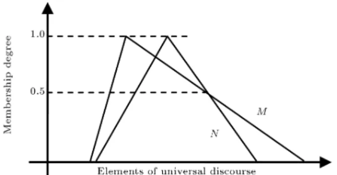
To choose the best path, the PTT values of all possible choices should be compared. The next issue is choosing an appropriate operator to rank fuzzy numbers. In this paper, Dubois and Prade's method for ranking fuzzy numbers using the possibility theory [18] is utilized. Their method is used to compare PTTs between a distinct origin and destination for dierent paths and to select the best path. For comparison, Dubois and Prade used both the possibility and the necessity theory. Supposing that \M" and \N" are two fuzzy numbers dened by two triangular MFs, Dubois and
Prade dened four indices: I1(M) = Poss (M N);
I2(M) = Poss (M < N);
I3(M) = Nec (M N);
I4(M) = Nec (M < N): (10)
Poss and Nec stand for possibility and necessity, re-spectively. Schematic denitions of these indices are shown in Figure 2.
As Figure 2 illustrates, I1(M) is the intersection
point of [N; +1) and the left side of \M"'s MF. More details about these indices are described in Henn [19].
The question may then arise as to \which of these indices is appropriate for the purpose of the shortest path when PTT is assigned to each link?" First of all, this index should discriminate between a fuzzy number (uncertainty) and a crisp number (certainty), otherwise the use of fuzzy numbers instead of deterministic travel time is meaningless. To see which of these indices has the above trait, some investigation is needed. For example, two fuzzy numbers \M" and \N" that represent the travel times on two parallel paths are compared. As shown in Figure 3, \N" is a singleton fuzzy number (displayed as line \bd"), and \M" is a fuzzy number with a triangular MF (displayed as triangle \acd").
The four indices for these two sample fuzzy numbers are as follows:
I1(M) = I1(N) = 1;
I2(M) = I3(N) = 1;
I3(M) = I2(N) = 0;
I4(M) = I4(N) = 0: (11)
Based on the indices I1 and I4, there is no dierence
between M and N; however, indices I2and I3indicate
that these two fuzzy numbers are dierent. This means that I1and I4do not take any uncertainty into account.
Yet, the aim of the fuzzy denition of PTT is to consider uncertainties, thus, these two indices do not meet our purpose.
The path with a PTT of \N" has a specic travel time, but the travel time of the other path with a PTT of \M" is uncertain. Path N is the best choice for a risk-averse driver; however, the path with uncertainty in travel time, M, is the best choice for a risk-seeking driver. The risk-seeking driver thinks that it is advantageous to reduce travel time by selecting the uncertain path, because by taking route M, there is the possibility that travel time will be less than route N. The risk-averse driver does not take the risk and selects path N to avoid potential excessive travel time in route M. Regarding this kind of behavior for risk-seeking and risk-averse users, I2 and I3 are appropriate for these
drivers, respectively, because in the system of I2, M is
the best choice and based on I3, N is better than M.
As a result, indices I1 and I4 only consider expected
travel time (the center of the PTT MF); however, the other two indices I2 and I3 also account for PTT
uncertainties and are, respectively, appropriate for risk-seeking and risk-averse drivers. Henn points out how the indices are sensitive to some parts of the MFs [19]. Figure 4 indicates that index I2 is used to compare
the left sides of the MFs and I3 is used to compare
Figure 3. Fuzzy numbers \M" and \N".
Figure 4a. Eective MF parts based on index I2.
Figure 4b. Eective MF parts based on index I3.
the right sides. This is intuitive when one knows that risk-averse decision makers choose an alternative in a pessimistic manner and use the right part of cost MFs in making their decision. Similarly, risk-seeking decision makers make choices based on the left part of the cost MF.
In reality, if a path's PTT uncertainty increases, then the proportion of trac using this path de-creases [16]. Because I3describes a person who avoids
uncertainty at the right part of travel time MF, it turns out that the index I3 can be appropriately used to
compare the PTT MFs of certain paths in order to select the best one.
A combination of index I3 and the way a MF
is constructed will eventually lead to a case in which drivers choose, from between two links, the link with a lower degree of saturation when the expected travel times (centers of the MF) are equal for both. According to the PTT MF denition in the previous section, if two links have equal expected travel times (i.e. the same center value in their MFs) but dierent degrees of saturation, then the links' MF limits will be dierent. The link with the higher degree of saturation has a lower left limit and a higher right limit. On the other hand, a person who is in the I3 category
will not prefer the choice with the higher right limit or, in other words, the link with higher degree of saturation, when the expected travel times are the same. For a person with an I2 index, the path with
more congestion is preferable; therefore, this is another indication that the I3 index should be used for the
purpose of shortest path determination in a congested network.
Although I3 is selected for use in the FSPA for a
network with congestion, the FSPA is also applicable to a risk-seeking individual; therefore, the values of indices I2 and I3 for two triangular fuzzy numbers
are computed. Suppose that M = (mL; m; mR) and
N = (nL; n; nR) are two fuzzy numbers. According to
Figure 2, I2(M) is the cross-point of ( 1; N[ and the
left side of the \M" MF. The membership degree of ( 1; N[ and left side of the \M" MF are determined
as follows: ( 1;N[=
8 > < > :
1 if x nL
n x
n nL if nL< x < n
0 if x n
(12)
M(x < m) =
(
0 if x < mL x mL
m mL if mL< x < m
(13) Index I2 is computed as follows:
I2(M) = n m
L
(m + n) (mL+ nL): (14)
Similar to the above computation, the values of index I3 for \M" and \N" are determined as follows:
I3(M) = n
R m
(mR+ nR) (m + n): (15)
It is assumed that when the indices for the two fuzzy numbers \M" and \N" are equal, \M" and \N" are also equivalent. For example, if I2(M) = I2(N), then
based on the value of index I2, \M" is as preferable as
\N". For two fuzzy numbers, \M" and \N", we also have [19] the following:
I2(M) + I2(N) = 1;
I3(M) + I3(N) = 1: (16)
Thus, we can say that if \M" and \N" are equivalent, then:
I2(M) = I2(N) = 0:5;
and:
I3(M) = I3(N) = 0:5:
Based on the index denitions, if the left side cross-point of \M" and \N" is equal to 0.5, then the two numbers are also equivalent by index I2. A similar
deduction for the right cross-point of \M" with \N" is true for index I3. Figure 5 shows the MFs of \M" and
\N" for the two situations.
So far, I3 has been selected for the comparison
of fuzzy numbers, the numerical value of I3 has been
computed for a general case, and it was shown that this index takes the degree of saturation in route choice into consideration when expected travel times of the routes are equal. The rest of this section describes how I3
aects the PTTs of several parallel paths where both the degree of saturation and expected travel time of the routes are dierent. To accurately identify how index I3 is used to compare dierent MFs, an example is
presented. Consider Figure 6, which shows the right
Figure 5a. Two equivalent fuzzy numbers based on index I2.
Figure 5b. Two equivalent fuzzy numbers based on index I3.
sides of the MFs for four fuzzy numbers A, B, C, and D. Despite their diering right limits, these fuzzy numbers are considered equal based on I3, because the
cross point of the right hand sides of these MFs is the same and equal to 0.5.
However, the expected travel time (MF center) and the travel time uncertainty (the MF right limit) increase and decrease, respectively, as one examines the MFs for \A" to \D" sequentially. It is obvious that I3
simultaneously takes into consideration the expected travel time and uncertainty in the risk-averse situation when comparing two fuzzy numbers.
The computational view of two equivalent fuzzy numbers based on I3 is as follows.
Using Equations 15 and 16, we can compute I3(N):
I3(N) = 1 I3(M) = 1 n R m
(mR+ nR) (m + n)
= mR n
(mR+ nR) (m + n): (17)
Two given fuzzy numbers \M" and \N" are equivalent, if I3(M) = I3(N), therefore, the following holds:
I3(M) = I3(N) , n R m
(mR+ nR) (m + n)
= (mR+nmRR) (m+n)n ,nR+n=mR+m:
(18) Similar to the above reasoning, we can also say, based on I3, that \N" is less than \M" if and only if nR+n <
mR+ m.
FUZZY SHORTEST PATH ALGORITHM (FSPA)
The proposed FSPA is similar to the Dijkstra algo-rithm, which uses a labeling procedure [20]. The FSPA is capable of nding the shortest path in an urban transportation network, in which the PTT is a fuzzy number assigned to each link.
The FSPA uses the I3 index described in the
previous section to compare parallel link PTTs and to choose the shortest path. First, it is necessary to dene the FSPA parameters:
V = the set of all nodes, S = the set of labeled nodes,
S = the set of unlabeled nodes, ~(zv) = the fuzzy length (fuzzy travel
time) of link (z; v), ~
d(v) = the fuzzy length from the origin to the node v (current node),
l(v) = the node before v in the shortest path from the origin (previous node),
i = algorithm step counter,
T = the tree Graph from s,
s = the origin,
zi= (i + 1)th labeled node,
neighbor(zi) = the set of nodes that connect to
node zi with only one link.
The algorithm is as follows: Step 1- Initialization:
Set: ~
d(s) = (0; 0; 0); S = fsg;
S = V fSg; z0= s; i = 0:
Set: ~
d(v) = 1; l(v) = s; 8v 6= s: Step 2- Update S, S and ~d(v):
2-1- ~d(v) = minf ~d(v); ~d(zi) + ~(ziv)g
8v 2 S \ neighbor(zi):
If: ~
d(v) = ~d(zi) + ~(ziv);
then: l(v) = zi:
2-2- Find zi+1 such that:
min
v2Sf ~d(v)g = ~d(zi+1):
2-3- S = S [ fzi+1g, S = S fzi+1g.
Step 3- If i = n 1 stop, else i = i + 1 and go to step 2.
Note: The function min computes the minimum of the fuzzy numbers according to index I3.
There are two points that need to be made about this algorithm if we intend to use it to nd the solution for a network with fuzzy travel time. First, all links coming to a labeled node, except for the shortest, will be ignored in future steps. For example, take the sample network shown in Figure 7 in which node \A" is a labeled node, and assume that link \1" travel time is less than link \2" travel time.
Using the conventional Dijkstra algorithm, which has a deterministic travel time for each link, we might claim that link \2" is ignored until the end of the algorithm because we can easily show that the shortest path from origin \O" to destination \D" does not contain link \2". This characteristic should also hold true for routes with a fuzzy travel time and a triangular MF to ensure that the labeling algorithm gives the best path between each origin and destination. Sec-ond, the proposed FSPA similar to those from other references [1,17] assumes that users include a shared link's travel time in the total travel time of a path when
Figure 8. Routes from origin \O" to destination \D" with a shared link.
comparing all paths between an origin/destination pair. For example, consider the network shown in Figure 8.
It seems that in reality users only compare routes based on the unique links within the routes. In other words, shared links should not have any eect on the nal decision. According to the above example, this means that a driver chooses the shortest path from \O" to \D" by comparing the travel time of the possible routes and ignoring link \AB" because it is commonly shared by all routes from \O" to \D". However, in Dijkstra's shortest path algorithm, the total travel time from origin to destination is computed at each step and includes the time spent in shared links for all routes. The shortest path obtained by users (when not considering shared links) and the Dijkstra algorithm will be the same if the travel time is assumed to be deterministic, however, in fuzzy circumstances, this result should be further reviewed.
In order to show that the above two points hold true under fuzzy circumstances, it is sucient to prove that if fuzzy travel time \A" is less than \B", then the summation of \A" with another fuzzy number, such as \C", is also less than the sum of \B" and \C". In other words, the following relationship (Lemma 2) should be proven:
A B , A + C B + C: (19)
It is possible to prove that this relationship is true when the I3 index is used to compare fuzzy travel times.
Before presenting the proof for Lemma 2, we need to rst prove Lemma 1.
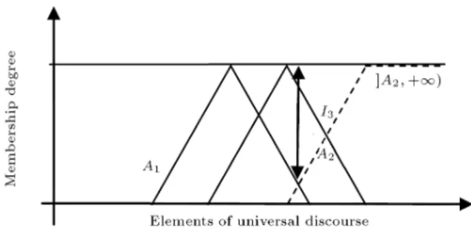
Lemma 1
The alternative \A1" is the best alternative between n
alternatives if, and only if, I3(A1) 0:5.
Without a loss of generality, assume that the best alternative corresponds to the shortest path.
Proof
Proof by contradiction:
(a) Suppose that \A1" is the best alternative, but
I3(A1) < 0:5 (contradiction hypothesis). I3(A1)
is equal to:
minfN(A1 A2); N(A1 A3); ;
N(A1 Ai); ; N(A1 An)g:
According to the contradiction hypothesis, at least one alternative like \Ai" exists, such that:
I3(A1) = N(A1 Ai) < 0:5: (20)
Because:
N(A1 Ai) + N(Ai A1) = 1;
then:
N(A1 Ai) = 1 N(Ai A1) < 0:5
)N(AiA1)>0:5>N(A1Ai): (21)
The above equation shows that there is an al-ternative named \Ai" that is better than \A1".
This result is in clear contradiction with the rst hypothesis, so that the contradiction hypothesis is invalid.
(b) Conversely, suppose I3(A1) 0:5 but the
alter-native, \A1", is not the best alternative
(contra-diction hypothesis). Thus there is an alternative with i 6= 1, such that \Ai" is the best alternative.
Therefore:
N(Ai A1) > 0:5 ) N(A1 Ai) < 0:5: (22)
We know that:
I3(A1) = minfN(A1 A2); N(A1 A3);
; N(A1Ai); ; N(A1An)g; (23)
I3(A1) = N(A1 Ai) < 0:5: (24)
Therefore, I3(A1) < 0:5. This result is in clear
contradiction to the rst assumption (I3(A1)
0:5), so it follows that the alternative, \A1", is
the best one.
Figure 9 claries Lemma 1. If A2 shifts to
the left on the X-axis, then I3 will decrease and,
when I3(A1) < 0:5, the fuzzy number, A2, will be
smaller than A1.
Now, Equation 19 can be proven using the result from the lemma above.
Lemma 2
If \A", \B" and \C" are three fuzzy numbers with a triangular MF, then the following relation is true for index I3:
A B , A + C B + C: (25)
Proof
(a) A B ) A + C B + C The fuzzy numbers are shown as:
A = (aL; a; aR); B = (bL; b; bR);
C = (cL; c; cR):
It is known that:
N(A B) = (aR+ bbRR) (a + b)a 0:5: (26) It should be shown that:
N(A + C B + C)
= (bR+ cR) (a + c)
(aR+bR+2cR) (a+b+2c)0:5: (27)
Rewriting Equation 26 yields:
N(A B) = (aR+ bbRR) (a + b)a 0:5 ) (bR a) 0:5
[(aR+ bR) (a + b)]: (28)
If we add the value (cR c) to both sides of
Equation 28, we obtain: (bR a) + (cR c) 0:5
b(aR+ bR) (a + b)c + (cR c) ) (29)
) (bR+ cR) (a + c) 0:5
b(aR+ bR+ 2cR) (a + b + 2c)c )
(30) ) (bR+ cR) (a + c)
(aR+ bR+ 2cR) (a + b + 2c) 0:5: (31)
(b) A + C B + C ) A B.
Because all of the above relationships are re-versible, the inverse argument is simply proven. The proof is illustrated in Figure 10.
Finally, we should prove that the proposed FSPA truly nds the shortest path.
Proof of FSPA Truth
To show that the FSPA outcome is correct, we need to prove that ~d(zi+1) is the shortest path with a fuzzy
travel time from s to zi+1. The induction method and
contradiction are used to prove the algorithm. In the rst step of the FSPA, the shortest path between s and s (which is zero) is obtained. Now, suppose in a middle step that the length of the shortest path from s to all nodes, available from V S, has been obtained and that zi+1 is a node labeled at the i + 1
step. The contradiction hypothesis shows that the minimum perceived travel time is not equal to the one obtained for the zi+1 node at the i + 1 step. In
other words, in the true shortest path from the origin to zi+1 there is a node, say v, which has not yet
been labeled. The mathematical translation of the contradiction hypothesis is below:
Nb ~d(v) + ~(vzi+1) ~d(zi+1)c > 0:5: (32)
Because a link travel time cannot be negative, we can write:
N[(0; 0; 0) ~(vzi+1)] 0:5:
Using the Lemma 2 result, we can write:
Nb ~d(v) ~d(v) + ~(vzi+1)c 0:5: (33)
The contradiction hypothesis and Equation 33 result in:
Nb ~d(v) ~d(zi+1)c > 0:5: (34)
On the other hand, because zi+1 has been labeled
before v:
Nb ~d(zi+1) ~d(v)c > 0:5: (35)
The two last equations (Equations 34 and 35) are in clear contradiction, so the contradiction hypothesis is invalid.
FSPA APPLICATION FOR A REAL NETWORK
The FSPA was applied to trac assignment on a real-world large-scale transportation network in Mashhad, one of the largest cities in Iran. Mashhad city is divided into 141 trac zones and it has a street network with 935 nodes, 2538 links and 7157 origin-destination pairs with non-zero observed demand. An origin-destination survey was conducted through at-home interviewing. Data were gathered from 4% of the households and validated through the observation of several screen lines in the study area. The trac volume for 118 links was recorded as part of the data gathering eort [21].
Figure 10. Illustration of Lemma 2.
The FSPA was implemented in a computer pro-gram using C++ language and run on a computer with a Pentium 4, 1.80GHz Central Processing Unit (CPU) PU and 512 megabytes (MB) of computer RAM memory. The shortest paths between all nodes in the Mashhad network were identied in less than one minute.
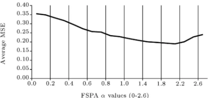
The link volumes were computed using an incre-mental assignment algorithm. For each step of the incremental assignment, the FSPA was used to nd the shortest paths. Then, the results were compared with the observed volume of the links. Figure 11 illustrates the accuracy of the assignment results compared to the observations using an increasing value.
The average Mean Square Error (MSE), which is used to compare the assignment results of the FSPA, using an increasing value, was computed using the following equation:
Average MSE =
n
P
i=1(OVi EVi) 2
n ;
where:
OVi= observed volume of link \i",
EVi= estimated volume of link \i",
n= number of links.
In this comparison, the volumes of 118 available ob-served links of the Mashhad network were compared to
Figure 11. Average Mean Square Error (MSE) for dierent values in FSPA.
the assigned volumes. The assignment algorithm used the FSPA for dierent values ranging from 0 to 2.6. For = 0, the assignment algorithm is the same as the traditional incremental assignment algorithm used by Dijkstra's shortest path algorithm. As Figure 11 indicates, as the value increases, the average MSE decreases. The average MSE continues to decrease until = 2:0. To minimize the MSE, = 2:0 is optimal, therefore, it is used to dene the membership functions for the Mashhad network link travel times. The travel time, for example link \a", will be shown using the following three parameters:
~ta= (tl= t0a; tc= ta(xa); tr= ta[3 xa]);
where ~ta, t0a, ta(xa) are the PTT, free ow travel
time, and travel time function for link \a", respectively. Because is greater than 1 and the left boundary cannot be a negative number, it is assumed that the free ow travel time is equivalent to the minimum lower bound for the link travel time. The upper bound of the travel time is equal to the link travel time when the link volume is three times its observed volume.
To assess the applicability of the FSPA to trac assignment, the results of the assignment using an incremental method with the FSPA are compared to the results of the UE assignment, as well as to a stochastic loading method, called Dial's assignment algorithm. Three graphs, shown in Figure 12, were used to compare the three assignment algorithms. The X-axis of these graphs corresponds to the estimated assigned volume and the Y -axis corresponds to the ob-served volumes. A trend line passes through the points, and the R2 value, as well as the trend line equation,
is included in the gures. As R2 approaches 1, the
accuracy of the estimated volume compared to the ob-served volume increases. It is expected that the trend line coecient and constant will approach 1 and 0, respectively. The trend line equation formed using the assigned volumes from the FSPA through incremental assignment algorithm has a better t to the theoretical values than the other two trend line equations. As shown in Figure 12, the volumes assigned using the
Figure 12. Comparison of the observed volume for links using (a) assigned volume by UE assignment with usual shortest path, (b) assigned volume by UE assignment with FSPA and (c) assigned volume by Dial's algorithm.
incremental assignment algorithm with the FSPA are the most accurate when compared to the observed volumes for 118 selected links. Consequently, the use of perceived travel times instead of denite travel times will increase the accuracy of the assignment model.
The computational platform for the three algo-rithms is the same. The assignment processing times were not considerably dierent between the algorithms. The results show the applicability of the FSPA for trac assignment in real transportation networks. CONCLUSION
This paper develops a FSPA for transportation net-works, in which travelers' perceived travel times are
assigned to links as fuzzy numbers dened using mem-bership functions. Fuzzy theory appropriately takes into account the uncertainty embedded in travelers' perceptions of travel times; however, fuzzy logic and arithmetic are, to some extent, complicated. Because travelers use their perceived travel times for links in their route choice process, the chosen FSPA should be ne-tuned for traveler route choice modeling.
The aggregation of all travelers' route choices within a transportation network results in a trac assignment that is traditionally computed using an assignment method such as a User Equilibrium (UE) or stochastic loading algorithm like Dial's assignment algorithm. In order to assess the applicability and per-formance of the resulting FSPA for trac assignments, the results of the assignment, using an incremental method that incorporates FSPA, are compared to the results of an UE assignment, as well as to Dial's as-signment algorithm for a large-scale real network. The comparison showed that an incremental assignment using our FSPA is the most accurate.
REFERENCES
1. Chang, P. and Lee, E. \Fuzzy decision networks and deconvolutions", Computers and Mathematical with Applications, 37(11-12), pp. 53-63 (1999).
2. Okada, S. and Soper, T. \A shortest path problem on a network with fuzzy arc length", Fuzzy Sets and Systems, 109(1), pp. 129-140 (2000).
3. Okada, S. \Fuzzy shortest path problems incorporating interactivity", Fuzzy Sets and Systems, 142(3), pp. 335-357 (2004).
4. Blue, M., Bush, B. and Puckett, J. \Unied approach to fuzzy graph problems", Fuzzy Sets and Systems, 125(3), pp. 355-368 (2002).
5. Chuang, T. and Kung, J. \The fuzzy shortest path length and the corresponding shortest path in a net-work", Computers and Operation Research, 32(6), pp. 1409-1428 (2005).
6. Moazeni, S. \Fuzzy shortest path problem with nite fuzzy quantities", Applied Mathematics and Computa-tion, 183(1), pp. 160-169 (2006).
7. Ji, X., Iwamura, K. and Shao, Z. \New models for shortest path problem with fuzzy arc length", Applied Mathematics Modeling, 31(2), pp. 259-269 (2007). 8. Hernandes, F., Teresa Lamata, M., Verdegay, J.L.
and Yamakami, A. \The shortest path problem on networks with fuzzy parameters", Fuzzy Sets and Systems, 158(14), pp. 1561-1570 (2007).
9. Teodorovic, D. and Kikuchi, S. \Transportation route choice model using fuzzy inference technique", First International Symposium on Uncertainty Modelling and Analysis, Ayyub, pp. 140-145, (1990).
10. Murat, Y.S. and Uludag, N. \Route choice modelling in urban transportation networks using fuzzy logic and
logistic regression methods", Journal of Scientic and Industrial Research (JSIR), 67(1), pp. 19-27 (2008). 11. Binetti, M. and De Mitri, M. \Trac assignment
model with fuzzy travel cost", 13th Mini EURO Con-ference Handling Uncertainty in the Analysis of Trac and Transportation Systems, pp. 805-812 (2002). 12. Arslan, T. and Khisty, C.J. \A rational approach to
handling fuzzy perceptions in route choice", European Journal of Operational Research, 168(2), pp. 571-583 (2006).
13. Zadeh, L. \Discussion: Probability theory and fuzzy logic are complementary rather than competitive", Technometrics, 37(3), pp. 271-276 (1995).
14. Zadeh, L. \Fuzzy logic = computing with words", IEEE Transaction on Fuzzy Systems, 4(2), pp. 103-111 (1996).
15. Ross, T.J., Booker, J.M. and Jerry Parkinson, W. \Fuzzy logic and probability applications: Bridging the gap", Society for Industrial and Applied Mathematics, 1st Ed., Philadelphia, pp. 18-20 (2002).
16. Henn, V. and Ottomanelli, M. \Handling uncertainty in route choice models: from probabilistic to possi-bilistic approaches", European Journal of Operational Research, 175(3), pp. 1526-1538 (2006).
17. She, Y., Urban Transportation Networks: Equilib-rium Analysis with Mathematical Programming Meth-ods, Englewood Clis, NJ, Prentice-Hall, 1st Ed. (1985).
18. Dubois, D. and Prade, H. \Ranking fuzzy numbers in the settings of possibility theory", Information Science, 30(2), pp. 183-224 (1983).
19. Henn, V. \Fuzzy route choice model for trac assign-ment", Fuzzy Sets and Systems, 116(1), pp. 77-101 (2000).
20. Xu, M., Liu, Y., Huang, Q., Zhang, Y. and Luan, G. \An improved dijkstra's shortest path algorithm for sparse network", Applied Mathematics and Computa-tion, 185(1), pp. 247-254 (2007).
21. Poorzahedi, H., Kermanshah, M., Ashtiani, H.Z. and Shafahi, Y. \Trac assignment model and Mashhad
transportation network performance in 1994", Sharif University of Technology, Institute of Transportation Studies and Research, submitted to Mashhad Munici-pality (1997).
BIOGRAPHIES
Hani Ramazani earned his BS degree (2005) in Civil Engineering and MS degree (2007) in Transportation Engineering and Planning, both from Sharif University of Technology, Tehran, Iran. He is now a PhD candi-date in Transportation Engineering at the University of Illinois at Urbana-Champaign, IL, USA. He is involved in ongoing projects related to trac operation and safety issues in highway work zones. His research interests include: Analysis of Highway Bottlenecks in Oversaturated Conditions, Eects of ITSs on Trac Operation and Safety, and Application of Articial Intelligence in Transportation Engineering.
Yousef Shafahi got his BS (1985) from Shiraz Uni-versity, Iran, a MS (1988) from Isfahan University of Technology in Iran and his PhD (1997) from the University of Maryland in the USA. He is now a Faculty Member of the Civil Engineering Department of Sharif University of Technology, Tehran, Iran. His research interests include: Transportation Modelling and Simulation, Urban Transportation Planning, Air Transportation, Road and Railway Engineering, and Application of Operation Research in Transportation Engineering.
Seyedehsan Seyedabrishami completed his BS (2003) in Civil Engineering and MS (2005) in Trans-portation Engineering and Planning, both from Sharif University of Technology, Tehran, Iran, where he is now nishing his PhD studies in Transportation Engineering and Planning. His research interests include: Forecasting Travel Demand and Fuzzy Theory Application in Transportation.