Rayan: A Polyhedral Grid Co-located
Incompressible Finite Volume Solver
(Part I: Basic Design Features)
M. Sani
1and M.S. Saidi
1;Abstract. In this work, basic design features of Rayan are documented. One of the new design features presented in this work is the way Rayan handles polyhedral grids. Grid denition is combined with the denition of the structure of the sparse coecient matrix, thereby releasing a considerable part of the memory used by the grid to store otherwise required faces belonging to the cell part of the connectivity description. The key idea is to use a uniform way for creating the structure of the coecient matrix from the grid connectivity description and to access that data when computing the elements of the coecient matrix. This saving requires many modications to the computational algorithm details, which are addressed. Computational method features include a SIMPLE-based pressure-velocity coupling and co-located variable arrangement in which all ow variables are stored at cell centers, and mass uxes are stored on face centers. Also handling convective and diusive uxes is described. The throughput is benchmark validated and shows second order truncation properties, both in time and space.
Keywords: Arbitrary polyhedral; Unstructured; Unsteady; Incompressible; Co-located.
INTRODUCTION
Numerical algorithms for ow simulation in complex geometries have evolved from Cartesian grid solvers to multi block [1-3], hybrid [4,5] and current state-of-the-art polyhedral grid solvers [6-12]. Solvers with polyhedral grid capability are appealing in complex ge-ometries. Arazgaldi [13] presents a cavitating propeller modeled using polyhedral grids. Polyhedral grids oer higher degrees of exibility, not only in mesh genera-tion, but also in grid adapgenera-tion, grid fusion (in multi grid) and overset grid applications. There are a variety of unstructured grid nite volume strategies. The rst choice to make is between cell-centered [8,11,14-17] or vertex-centered schemes [14,18-20]. This work is just concerned about the cell-centered methods. The variable arrangement is also a matter of consideration; without going into the details, we use the widely used co-located variable arrangement.
Another important thing about the unstructured
1. Center of Excellence in Energy Conversion, School of Mechanical Engineering, Sharif University of Technology, Tehran, P.O. Box 11155-9567, Iran.
*. Corresponding author. E-mail: mssaidi@sharif.edu
Received 5 January 2010; received in revised form 11 July 2010; accepted 16 August 2010
grid is the way its connectivity is dened. There is no counterpart for connectivity in structured grids because it is implied by indexing. Unfortunately, connectivity requires the major part of the memory consumed for unstructured grid handling. In FEM applications it is preferred to use element-based or edge-based connectivity (see for example [21]). The element-based (cell-based) connectivity describes the connectivity as a nodes belonging to cell relationship. For FVM, however, because of the need to compute uxes over the faces of each cell, face-based connec-tivity is preferred. Face-based connecconnec-tivity also allows for uniform implementation of the arbitrary polyhedral grids, because it does not need any special treatment for dierent cell topologies. The face-based connec-tivity has two parts: nodes belonging to a face and faces belonging to a cell (F2C). A modied version of the face-based connectivity adds a Left and Right Cell (LRC) relationship for each face. This inclusion adds to the storage cost but removes the search overhead for interpolation to face centers. The connectivity description method chosen directly aects the way elements of the coecient matrices are evaluated.
There is extensive literature concerning dis-cretization of the terms (like convection term) in the governing integral equations, their accuracy and their
stability. At the same time, ecient use of the computational hardware was always of concern. Nowa-days, with lower hardware costs, simulation of ner details and more complex physics are possible. Even coupled solvers with much larger coecient matrices than segregated ones are becoming attractive [22]. The trend is to consume all resources available to capture more details and handle more realistic cases. This encourages continuous development of more ecient computational methodologies.
In this work, we rst describe one methodology for discretizing incompressible ow equations on poly-hedral grids (a technology frontier by itself). Then, we show that there is a potential for memory saving by changing the strategy of computing coecient matrix elements. The proposed modication removes the need for F2C, which is a heavy memory burden in the face-based connectivity description. Assuming that there are Ncells cells in the domain and, on average, Nf faces per cell, the memory consumed by F2C is equal to Ncells Nf integer values. If, on average, there are Nv vertices per face and a total of Nfaces in the domain, the total memory occupied by the connectivity is Nfaces Nv+ Ncells Nf+ 2 Nfaces integers (the last term describes the LRC requirement). Table 1 shows the memory share of the F2C relative to the total memory required by the connectivity and grid (node coordinates plus connectivity) for dierent un-structured grids lling two- and three-dimensional unit cavities with cell edge sizes equal to 0:05. The share is always larger than 22% and the saving potential is considerable.
The major contribution of this work is to propose a method to combine features of the face-based connec-tivity and structure of the sparse coecient matrix for evaluating coecient matrix elements without impos-ing search or storage overheads and without requirimpos-ing the F2C part of the connectivity. To completely remove the need for storing F2C, many details like the way the gradient or geometric entities are computed need reconsideration, which is also addressed.
In what follows, rst the details of a polyhedral grid discretization is given. This shows why F2C is required in common practice. Then, by dening cell-based and face-cell-based jobs, it is shown that the need for F2C can be removed. In the next section, geometric entities and elements of the coecient matrix are
computed without invoking F2C data. Finally, some benchmark problems are solved to test the integrity of the methodology and validate its correct truncation error behavior.
POLYHEDRAL GRID DISCRETIZATION OF THE GOVERNING EQUATIONS
For the incompressible ow, the continuity and momen-tum equations are:
Z
~V :d~S = 0; (1)
@ @t
Z
dV +
Z
(~V :d~S) = Sp+ Z
D@@ndS +
Z
qVdV; (2)
where could be any transported scalar including velocity components (u, v, w), qV is the volumetric
source term and Sprepresents the pressure term, which is only applicable to the momentum equations as:
~Sp= Z
~rpdV =
Z
pd~S: (3)
Sign and Naming Conventions
Before going into the details of discretization, it is convenient to put forward some conventions. There are two cases where the face direction is required, with regards to a cell and independent. With regards to a cell, j is used for the face number and the positive direction is always outwards from the cell. In independent addressing, the face vector, ~Sf, is dened by the order of its vertices (nodes) and the right hand rule. In this case, f is used to address the face number. There are two cells sharing a face, P0f and P1f, chosen so that the face vector, ~Sf, points from the left cell, P0f, to the right cell, P1f. Figure 1 illustrates these conventions.
Implicit Time Discretization
For integration in time, we follow the implicit second order three time levels method. The unsteady
equa-Table 1. Comparison of the memory share of F2C for dierent unstructured grids in unit square (cube in 3D). Grid edge size is set equal to 0:05 for all of the cases. Single (double) denotes single (double) precision.
F2C Share Quad. Tri. Hexa (3D) Tetra (3D) Wedge (3D)
Connectivity 32% 33% 30% 28% 26%
Grid (Single) 27% 29% 26% 27% 24%
Figure 1. Polyhedral cell terminology. Also shown is the division of the highlighted face to triangles for geometric computations.
tions are symbolically rewritten as: dy
dt = H; (4)
where y represents the volume integral in Equation 2 and H contains all other terms. Discretization gives:
3yn 4yn 1+ yn 2
2t =
dy
dt n
+ O(t2)
= Hn+ O(t2): (5)
Applying the above time discretization, Equation 2 could be discretized in space for a polyhedral cell, P0, having Nj faces to:
aP0P0+
Nj
X j
aPjPj = bP0; (6)
in which aP0, aPj and bP0 carry the eects of implicitly
or explicitly discretized integrals. Volume Integrals
The volume integrals are discretized to second order using the mid-point rule:
Z VP0
dV P0VP0: (7)
Convection Terms and Mass Flux Computation Convection surface integrals are discretized using the mid-point rule as:
Z
j(~V :d~S) _mjj; (8)
where j represents the face center value and mass ux
is assumed positive out of the cell. To avoid pressure checker-boarding, the mass ux in Equation 8 is ob-tained from the standard Rhie-Chow [23] (momentum-based) interpolation between the cells which have face f in common as:
unf =
_mf
Sf = (~u)f:^nf +
V
a0 P nf
f
V
a0
f
P nf
f; (9)
where (:)f means any interpolation to the face center, like CDS, a0 is the main diagonal element in the dis-cretized momentum equation of the corresponding cell, and (:)=nf is the discretized face normal derivative operator.
To nd an approximation to j for Equation 8, any upwind scheme could be used. To promote the numerical stability of the solver, a deferred correction strategy [24] is used in this work. In this strategy, the standard First Order Upwind (FOU) is used for computing the coecient matrix, which gives it good iteration properties. To promote accuracy to second order, the dierence between FOU and the standard Second Order Upwind method (SOU) is added to the right hand side (i.e., lagged one iteration). The converged solution corresponds to SOU, while the coecient matrix behaves as good as FOU.
For FOU, the upwind cell must be identied rst. The upwind cell, PU, is determined using the direction of the mass ux relative to face normal vector (~Sf). The value of PU is assumed to be convected to the
face center (FOU
j PU). For SOU correction, the
value of at the face center is interpolated using PU
and (~r)PU. The face center value is approximated to
second order as: SOU
j PU+ (~r)PU:(~rj ~rPU): (10)
Diusion Terms
Diusion surface integrals are discretized using: Z
jD @
@ndS D
njSj: (11)
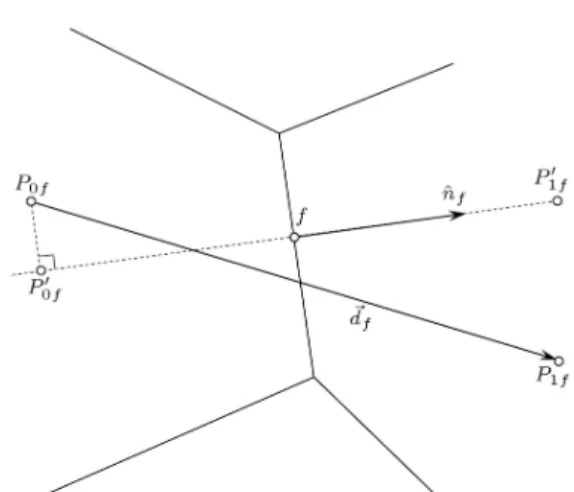
To approximate the normal derivative, virtual points are used. The virtual point in cell P0f related to face f is dened as the normal projection of the cell center on the face normal:
~rP0
0f = ~rf+ [^nf:(~rP0f ~rf)]^nf; (12)
where ^nf is the unit normal vector of face f (Figure 2). The virtual point in cell P1f is dened as the mirror image of the virtual point in P0f with respect to
Figure 2. Denition of the virtual points.
the common face. The line connecting virtual points P0
0f and P1f0 is orthogonal to the face, and passes through the face center just at the mid-point of the line. Therefore, to second order:
nf
P0
1f P0f0
j~rP0
1f ~rP0f0 j
= P1f0 P0f0
j~d0 fj
; (13)
where values at virtual points are obtained using gradient-based interpolation, e.g.:
P0
0f P0f + (~r)P0f:(~rP0f0 ~rP0f):
Pressure-Velocity Coupling
Continuity equation is used with SIMPLE algorithm to derive the pressure correction equation. For this algorithm, currently available velocity components and pressure are assumed to be predictions to the correct values, requiring a set of corrections which are related to each other as:
~u0 P0
VP0
a0 (~P 0)
P0; (14)
where ~ is the discrete gradient operator. Obtaining the required mass ux correction from the velocity cor-rections, and substituting in the discretized continuity equation gives the pressure correction equation for cell P0 as:
Nj
X j
V a0
j
(~P0) j:~Sj
! =
Nj
X j
( _mj) ; (15)
where (~P0)
j:~Sj is obtained using Equation 13 and: (~P0)
j:~Sj= P 0
njSj: (16)
This leads to a linear system of equations of the form: cP0PP00+
Nj
X j
cPjPP0j = dP0: (17)
Boundary Condition Application
To avoid special treatment for cells near boundaries, ghost cells are used outside the physical domain. Therefore, each boundary face, f, is surrounded by one real cell, P0f, and one ghost cell, PG. The ghost cell center is dened as the mirror image of the virtual point inside the real cell, P0
0f, with respect to the boundary face. With this choice, the face center value and the face normal derivative are easily computed to second order as:
f
PG+ P0f0
2 ; (18)
@
@nf
PG P0f0
j~rPG ~rP0f0 j
: (19)
Boundary conditions are considered as the governing equations for the ghost cells.
Gradient Computation
The above outlined discretization assumes a gradient vector to be available. It is computed using the standard least square method as outlined in [18]. Since, near any cell center, ~rP0, the value of can be
approximated to second order as:
(~r) P0+ (~r)P0:(~r ~rP0); (20)
neighbor cell center values, at ~rPj, can be obtained
from:
Pj = P0+ (~r)P0:(~rPj ~rP0)
= P0+ (~r)P0:~dj: (21)
Rearranging for the gradient gives:
(~r)P0:~dj= Pj P0: (22)
This is always an over determined system of equations for gradient components, since in three (two) dimen-sions, there are at least four (three) neighbors for each cell but three (two) components of the gradient are to be solved for. Following the standard least square procedure, the gradient components could be obtained as:
(~r)P0 = D 1
X j
dT
j(Pj P0); (23)
where, j runs over all of the neighbors of P0, dTj is the single column notation for ~dj and D is a symmetric three by three (two by two in 2D) geometry-dependent matrix dened as:
D =X
j dT
jdj = 2
4a b cb d e c e f 3
The inverse of D is computed analytically as:
D 1= 1
adf + 2bce ae2 dc2 fb2 2
4df e
2 ce bf be cd
ce bf af c2 bc ae
be cd bc ae ad b2
3
5 : (25)
Having geometry dependent D available, the gradient vector could be obtained from Equation 23. Since the computation of the gradient requires the knowledge of the neighbor values of , whenever the gradient is encountered in the discretization, it is lagged. This means that the values from the last iteration are used for the computation of the gradient. At convergence, this lagging will not aect the solution, but it may slow down the convergence.
Coecient Matrices and Their Storage
Following the routines outlined above, a linear system of equations of the form of Equation 6 is obtained for each of the velocity components. The coecients of the system are given in Table 2. It is evident that the coecient matrix is sparse with compact support (stencil extended just to immediate neighbors). The pressure correction discretized equation has the same structure with coecients given in the same table.
For the nite volume method described above, non-zero elements are related to the discretization of the volume and surface integrals. Volume integrals aect the main diagonal elements, while surface in-tegrals, because of the required interpolations, aect both main and o-diagonal elements. Every row in the coecient matrix (row i) corresponds to the discretized transport equation for cell number i. Therefore, non-zero elements on the ith row are just on the main diagonal or at the column numbers corresponding to the cell number of the neighbors of the ith cell.
Sparse coecient matrices can be economically handled with a common Compressed Row Storage format (CRS). In CRS, non-zero members of the coecient matrix are sequentially stored in a one-dimensional array, a, swapping the matrix row by row. The column number of every non-zero element encountered is also stored in another one-dimensional array called colindex. For every row, a pointer to the beginning element of the row in a is stored in another one-dimensional vector called rowptr. This means that rowptr[i + 1] rowptr[i] is the number of non-zeros on the ith row of the original matrix. Non-zero values corresponding to that row are stored in a[rowptr[i]] to a[rowptr[i + 1] 1]. In the data chunk related to a row, the order is not important. For convenient access to the main diagonal element, we use the rst place of the data chunk to store the main diagonal element.
Usually, rowptr is extended by a single element, which stores the total number of non-zeros for the sake of uniformity of application. The interdependence of these three one-dimensional arrays and the grid is illustrated in Figure 3. It is worth noting that since non-zeros correspond to the neighbors, the structure of the coecient matrix could be obtained from the grid
Figure 3. The structure of the sparse coecient matrix and its relation to the grid topology.
Table 2. The elements of the coecient matrix resulted from the implicit discretization of the generic scalar transport Equation 6 and pressure correction Equation 17 on cell P0.
aP0
3(V )P0 2t +
PNj
j
max( _mj; 0) + Djj~j~Sdj0j jj
aPj min( _mj; 0) Dj
j~Sjj
j~d0 jj
bP0
4(V )P0()n 1
p0 (V )P0()n 2p0
2t + qP0VP0
+PNj
j
Djj~j~Sd0jj
jj
(~r)Pj:(~rP0
Pj ~rPj) (~r)P0:(~rPP00 ~rPP0)
old
+PNj
j max( _mj; 0)P0+ min( _mj; 0)Pj ( _mjj)SOU
old
cPj
V a0
j j~Sjj
j~d0 jj
cP0
PNj
j cPj
dP0
PNj
information without constructing the two-dimensional matrix itself (and paying for the associated high mem-ory costs).
Methods to Compute Coecient Matrix Elements
One easy way to compute the transport coecient matrix is to loop over all of the cells. For every cell (cor-responding row in the coecient matrix), computation of the main and o diagonal elements requires at least the knowledge of the volume of the cell, area of its faces and cell number of its neighbors. The volume of the cell is readily available because the cell number coincides with the row number of the coecient matrix. The area of the faces requires the cell to know its faces. This information is taken care of using the face belonging to cell (F2C) part of the connectivity. Neighbors of the cell are stored as Left and Right Cell (LRC) in the face-based connectivity. Therefore, if the cell knows its faces and if every face knows its adjacent cells, neighbor information is available to the cell.
Of course, although the above methodology pro-vides sucient means to evaluate the elements of the coecient matrix, it is by no means the most ecient way. It requires double computation of the face uxes (once per each cell sharing the face). It also requires the storage of the bulky F2C in the grid connectivity. Another problem with the method is nding the element on row number i with column number j in a sparse matrix. Fortunately, the or-der of storage of faces in F2C for each cell could be exploited to remove this search overhead. This order is not available in discretization without F2C. This work describes a way to circumvent this search problem.
To avoid double computations (per face), one can rst loop over all of the faces of the domain and compute the implicit and explicit uxes per face. The values cannot be directly inserted into the coecient matrix unless a search is undertaken to nd column number j on row number i in the sparse system. This time the order in F2C could not be exploited because looping over the faces of the domain makes it impossible to know the sequential place of the face number in the ordered F2C list of the corresponding cells, unless a search is carried out. Now that the direct insertion requires a search overhead, one may store the computed uxes per face. This requires a storage space proportional to the number of faces. By looping over the cells, these values could be retrieved (instead of computed) and used to ll the coecient matrix without searching (exploiting the order in F2C ).
To summarize, the three methods presented above require either added computational cost (double com-putations per face or search overhead to locate the
element in the spare matrix) or memory overhead (ux storage per face and F2C ).
CELL-BASED AND FACE-BASED JOBS A Cell-Based (CB) job is dened as a job which requires a loop over the cells in the computational domain. The rst process of evaluating the coecient matrix dened previously is an example of a CB job. Similarly, a Face-Based (FB) job is dened as a job which requires a loop over the faces in the computational domain.
As described previously, computing elements of the coecient matrix in a row by row (CB) manner not only requires F2C, but also demands that the uxes over the faces (surface integrals) be computed twice (once for each cell sharing the face). To remove this double computation overhead, one can rst dene a FB job in which all of the uxes are evaluated and stored per face. Then using a same CB job as before, the elements of the coecient matrix are evaluated. This time, since the uxes are available per face, they are just retrieved. This although removes the double computation overhead, requires a storage space equal to the number of faces for the uxes. To summarize, the aforementioned methodology is carried out with following steps:
1. Loop over all of the faces in the domain. For each face:
(a) Use LRC to interpolate to the face center and compute uxes.
(b) Store the ux for the face.
2. Loop over all of the cells of the domain. For each cell:
(a) Compute the eect of the volume integrals and update the main diagonal element.
(b) Use F2C to nd its faces. Loop over the faces of the cell. For each face:
i. Retrieve the value of uxes stored for the face.
ii. Insert the main diagonal element share from the face.
iii. Insert the o-diagonal element share from the face by retrieving the related neighbor cell number from LRC.
It is worth noting that the right hand side of each equation is treated in the same way as the main diagonal element.
DISCRETIZATION WITHOUT F2C
The other way, proposed in this work, is to evaluate and accumulate all of the uxes in the FB job. This not only removes the need for the ux storage, but also removes the need for F2C. The task is carried out as:
1. Loop over all of the faces in the domain. For each face:
(a) Use LRC to nd neighboring cells and interpo-late to nd face uxes.
(b) Directly insert the share of the face ux to the main and o diagonal elements of the coecient matrix.
2. Loop over all of the cells of the domain and insert the eect of volume integrals on the main diagonal elements.
The key step is Step 1b. Directly inserting the share removes the need for storage of the uxes for later use. It also removes the need for storage of F2C, since the CB job of Step 2 has nothing to do with faces of the corresponding cell and, therefore, does not require F2C. For inserting the shares in Step 1b, one needs to know the insertion location in the coecient matrix stored in CRS format (the same idea applies to other sparse storage mechanisms).
For face number f, there are two neighbor cells, namely, P0f and P1f. The ux over this face con-tributes to the main diagonal coecient of the equa-tions at row numbers P0f and P1f. It also contributes to the element located at column number P1f on row number P0f, and the element located at column number P0f on row number P1f. For full matrix storage, access to these elements is trivial. Of course, this is not the case when sparse storage is exploited (which is the economical way of handling unstructured-grid real-word problems).
The main diagonal element on row number i is stored in a[rowptr[i]] and is easily accessible. The o-diagonal element on row number i and column number j can be found as follows. The easiest, but not the most ecient, way is to search over the data chunk stored in colind[rowptr[i]+1] to colind[rowptr[i+1] 1] for j. The number of data stored there is equal to the number of faces cell number i has. Therefore, this is a low cost search for each cell. But it should be carried out many times for the whole grid, which imposes a search overhead. This overhead can be avoided as proposed below.
The key idea is that the order of cell numbers (column numbers in colind) depends on the way the structure of the coecient matrix is created from the grid connectivity description. If the same procedure is used for accessing that data, there is no need for a search. The structure of the coecient matrix is to be generated from a face-based grid description. Since the connectivity is to be described as node belonging to face and Left and Right Cells (LRC) of the face, one-dimensional arrays, a, colindand rowptr, are to be formed just using LRC.
The rst step is to reserve memory for them. The length of rowptr is equal to the number of rows of the
coecient matrix (equal to the number of cells) plus one: a and colind have equal lengths. Since they hold non-zero elements, their lengths are equal to Ncells+ 2Nfaces. Ncellsaccounts for the main diagonal elements and 2Nfacesrepresents the total number of o-diagonal non-zero elements. O-diagonal elements (cross-links) are the result of the inter-connection of the equations. For face number f, there is an o-diagonal element on row number P0f and column number P1f, and another o-diagonal element on row number P1f and column number P0f. Therefore, there are 2Nfaces o-diagonal non-zero elements.
The next step is to ll rowptr and colind, which together dene the structure of the sparse coecient matrix. For rowptr, since it stores the oset of the rst element of each row from the rst non-zero in the coecient matrix, we rst need to count the non-zeros on each row and then accumulate them:
1. Put one in every element of rowptr accounting for main diagonal elements.
2. Count o-diagonal elements: Loop over the faces of the domain. For every face, f, use LRC to nd neighboring cells (P0f and P1f) and increment the values stored in rowptr[P0f] and rowptr[P1f]. The reason is that every face means a cross-link between its left and right cells and this adds to the number of elements on the corresponding rows. After this loop, every rowptr[i] contains the number of non-zeros on the ith row of the coecient matrix. 3. Accumulate these values towards the end of the
rowptr in a loop over the elements of rowptr in order to nd the required oset. This is done in a loop from the second element of rowptr onwards; for every element, i, setting rowptr[i] to rowptr[i] + rowptr[i 1].
4. Shift all elements of rowptr towards the end by a loop from the last element to the second one, and, for each element i replace the current value by rowptr[i 1]. For the rst element, zero should be used.
Now every element in rowptr contains the number of non-zeros before the corresponding row in the coe-cient matrix.
To complete colindex, we make use of an auxiliary, one-dimensional integer array with NcellS elements called front. Since front and pressure correction (P0) are never required simultaneously, and since the memory for P0 must be reserved and is greater than or equal to the memory required by front, that space could be used which removes any memory overhead. The aim of using the front is to keep the track of the lled elements in colind for each row:
1. Main diagonal elements: In a CB job (with index i), put i in colind[rowptr[i]] which means that the rst
element of the data chunk related to the row num-ber i is the diagonal element with column numnum-ber i. At the same time put one in the corresponding elements of front, which means that for every element, one column index is set (the main diagonal one). After this step, all o the elements of front contain one.
2. O-diagonal column numbers: Loop over the faces of the domain. For every face f use LRC to nd neighboring cells (P0f and P1f). Set P1f in colind[rowptr[P0f] + front[P0f]] and increment front[P0f] (advance the front for P0f). Also set P0f in colind[rowptr[P1f]+front[P1f]] and increment front[P1f] (advance the front for P1f).
Mimicking Step 2 when computing elements of the coecient matrix makes it possible to insert the o-diagonal shares of the elements of the coecient matrix without search overhead.
It is now appropriate to separate the CB and FB shares of the elements of the coecient matrix. Table 3 shows this splitting. FB and CB superscripts stand for the face-based and cell-based shares, respectively. Also it is worth noting that symbols like (aP0f)P1f
mean the coecient of P0f in the equation related
to its neighbor with cell number P1f and therefore the
element on row number P1f and column number P0f of the coecient matrix.
Now elements of the coecient matrix are evalu-ated with:
1. Make all elements of the coecient matrix (ele-ments of a) zero.
2. Loop over all cells and add cell-based shares to the main diagonal and right hand side elements. For each cell put one into the corresponding element of the front.
3. Loop over all faces of the domain, for each face, f, retrieve P0f and P1f cells from LRC and add the contribution of the face to (aP0f)P1f, (aP1f)P0f,
(aP0f)P0f, (aP1f)P1f, bP0f and bP1f. After adding
the shares, advance the front for P0f and P1f (i.e., increment the values stored in front[P0f] and front[P1f]).
Step 3 requires the knowledge of the position of the elements in a. Element (aP0f)P1f is located
at a[rowptr[P1f] + front[P1f]]. Likewise, (aP1f)P0f is
located at a[rowptr[P0f] + front[P0f]]. Main diag-onal element (aP0f)P0f is located at a[rowptr[P0f]]
and (aP1f)P1f is located at a[rowptr[P1f]]. The same
method could be applied to the pressure correction
Table 3. Face-based and cell-based shares of the elements of the coecient matrix. FB shares are from face number f.
aF B P0f
P0f
max( _mf; 0) + Djj~j~Sdf0j fj
aF B
P0f
P1f
aF B
P0f
P0f
aF B
P1f
P1f min( _mf; 0) + Dj
j~Sfj
j~d0 fj
aF B
P1f
P0f
aF B
P1f
P1f
bF B
P0f
P0f
Dj
j~Sfj
j~d0 fj
(~r)P1f:(~rPP1f0 ~rP1f) (~r)P0f:(~rPP0f0 ~rPP0f)
old +max( _mf; 0)P0f+ min( _mf; 0)P1f ( _mjj)SOUP0f
old
+ qP0VP0
bF B
P1f
P1f
bF B
P0f P0f aCB P0 P0
3(V )P0 2t
bCB P0
P0
4(V )P0()n 1
p0 (V )P0()n 2p0
2t
cF B
P1f P0f V a0 j j~Sfj
j~d0 fj
cF B
P0f
P1f
cF B
P1f
P0f
cF B
P0f
P0f
cF B
P1f
P0f
cF B
P1f
P1f
cF B
P1f
P0f
dF B
P0f
P0f _mf
dF B
P1f
P1f
dF B
P0f
equation because the structure of the coecient matrix is the same.
Required Modications When F2C Is Not Available
Computing geometric entities like cell volume needs reconsideration when F2C is not available. Since the cell does not know its faces, the volume could not be obtained in a CB job. Assuming that the face area and center are available (which require no modication regarding the removal of F2C ) in CB oriented calculations, the cell volume could be obtained from Gauss's theorem as:
VP0=
Z VP0
dV =13 Z VP0
~r:~rdV = 13 Z SP0
~r:d~S
= 13 Nj
X j=1
~rj:~Sj: (26)
Or equivalently from: VP0=
Z VP0
dV = Z VP0
~r:(x^i)dV = Z SP0 (x^i):d~S = Nj X j=1
xj(^i:~Sj) = Nj
X j=1
xj(Sx)j: (27)
Cell volumes could be computed by accumulating FB shares while looping over all faces of the domain as:
8 > < > :
VF B
P0f = xf(Sx)f
VF B
P1f = xf(Sx)f = VPF B0f
(28) Computing cell centers also requires modication. Ac-cording to its denition, the x coordinate of the cell center could be computed from:
x:VP0 =
Z VP0
xdV = Z VP0
~r:(x22^i)dV
= 1 2
Z SP0
(x2^i):d~S = 1 2
Nj
X j=1
(^i:^nj) Z Sj
x2dS: (29) For each face, the last integral could be computed [25] from the triangulation of the face (Figure 1). For each triangle, a vertex is chosen as vertex number zero (~r0). The other two vertices are numbered in a right hand manner, so that their cross product is consistent with the face area vector direction. The relative location
vector of these vertices is computed as ~ei= ~ri ~e0. A surface parameterization of the triangle is assumed as ~r(p; q) = ~r0+ p~e1+ q~e2 constrained to 0 6 p; q 6 1 and p + q 6 1. With this parameterization, the surface mapping relationship is:
dS =@p@~r@~r@q = j~e1 ~e2jdpdq: (30) This results to:
(^i:^nf) Z Sf
x2ds = (~e
1 ~e2):^i 1 Z 0 1 q Z 0
(x(p; q))2dpdq: (31) The integral could be evaluated analytically as:
1 Z 0 1 q Z 0
(x(p; q))2dpdq = 1
12(x20+ x21+ x22
+ x0x1+ x0x2+ x1x2): (32)
The result of the integral when substituted in Equaiton 29 gives the cell center in terms of the nodal coordinates of its vertices. For a face-based application, the share of each cell from each face could be computed from: 8 > > < > > :
xF B
P0f = 2V1P0f(^i:^nf)
R Sfx
2dS
xF B P1f =
1
2VP1f(^i:^nf) R
Sfx
2dS
(33) Therefore, cell centers could be found by looping over all faces of the domain; for each face, computing the integral in Equation 33 by substituting the coordinates of its nodes into Equation 32 and adding the shares to left and right cells according to Equation 33.
Computation of the D matrix used for evaluating the gradient and stored at cell centers also requires reconsideration. Since from Equation 24, D is equal to PjdT
jdj, it could be computed in a FB job with face shares equal to:
DF B
P0f = DF BP1f = dTfdf: (34)
After that D is available at cell centers, it can also be inverted using Equation 25 in a CB job.
To compute gradient eld for from Equation 23 again a FB job followed by a CB job is employed. The share of each face inPjdT
j(Pj P0) is computed in
a FB job and is accumulated on the memory reserved for gradient vector at cell centers by:
(dT
j(Pj P0))F BP0f = (dTj(Pj P0))F BP1f
= dT
f(P1f P0f): (35)
Now in a CB job, D 1 can be multiplied to
P
jdTj(Pj P0) and stored at the same place for the
INTEGRITY AND ACCURACY CHECKS Using the methods outlined above, Rayan was de-veloped with object oriented design. To verify the integrity and check its accuracy, some benchmark problems were solved, as reported hereafter.
Lid-Driven Cavity Problem
The lid-driven cavity problem is a rst step standard test case for which a vast numerical and experimental data base exists. To verify polyhedral treatment, a grid was created with 3962 cells (7701 faces and 3740 vertices). It was a combination of quadrilateral (near wall) and triangular (center) cells (Figure 4). The ow was solved at Reynolds numbers ranging from 102 to 104. Also shown in Figure 4 are the streamlines corresponding to Re = 104. Even on such
Figure 4. Benchmark validation using cavity problem at Re = 104.
a course mesh, tertiary and quaternary vortices are captured on the left-bottom and right-bottom corners, respectively. Horizontal and vertical components of velocity on vertical and horizontal symmetry lines are compared to the benchmark values given by Ghia et al. [26]. Regardless of the coarseness of the mesh, results compare well with benchmark data, which were obtained on a 257 257 grid (17 times more nodes) using a multi-grid stream function-vorticity method. Decaying Vortices Problem
The decaying vortices problem, having an analytical solution, is commonly used to measure the order of accuracy of the codes. Upon substitution, it could be easily shown that the ow eld deed by:
8 > > > > > > < > > > > > > :
u(x; y; t) = cos(x)sin(y)e 22t=Re
v(x; y; t) = sin(x)cos(y)e 22t=Re
p(x; y; t) = 1
4(cos(2x) + cos(2y))e 4
2t=Re
(36) satises incompressible ow equations. This problem is solved for Re = 10 and in the range (x; y) 2 f 1
2 < (x; y) < 1
2g (following [4]). Analytical values are used as the boundary and initial conditions. The errors are computed at t = 0:3 (the time at which the maximum velocity decays to almost half of its initial value). Various norms of error are dened as:
"L1= P
jucomputed uanalyticj
Ncells ; (37)
"L2= sP
(ucomputed uanalytic)2
Ncells ; (38)
"L1= max(ucomputed uanalytic): (39)
To nd the order of the space discretization truncation error, the ow is solved on systematically rened uniform grids of 10 10, 20 20, 40 40 and 80 80 cells. The time step is held constant at 0:001. Since the time step is small, almost all errors could be related to the space truncation error. Figure 5a proves that the error (described by three norms) is indeed of second order in space.
To check the truncation error in time, the problem is solved on a 113 113 uniform grid with time steps of 0:1, 0:075, 0:05, 0:03 and 0:025. Because the grid is very ne and time steps are so large, the error could be related to the time series truncation. The error is shown in Figure 5b, which proves the method is of second order in time, as well.
Figure 5. Error for decaying vortices problem with respect to the analytical solution at t = 0:3.
Flow Passing a Circular Cylinder
Flow normal to a cylinder possessing vortex shedding is solved at Reynolds numbers of 200 and 1000 on the grid shown in Figure 6. The mesh is a combination of clustered body conforming quad cells near the cylinder and triangular cells covering the rest of the domain. The related Strouhal number, dened as
Figure 6. Domain and the mixed type grid used for the simulation of the vortex shedding problem over a cylinder.
Figure 7. Streamlines for ow passing a circular cylinder at Re = 1000 and t = 80.
Table 4. Comparison of the St numbers for the vortex shedding from a circular cylinder.
Manzari [27] He [28] Present StRe=200 0.20 0.1978 0.1980
StRe=1000 0.238 0.2392 0.2381
St = fD=V1, describes the frequency of the vortex shedding. Figure 7 show streamlines for t = 80 after sudden exposure to a ow with = 1 and = 0:001 owing at u = 1. Table 4 summarizes the results for Re = 200 and 1000. As is evident, St numbers are in close agreement with Manzari [27] and He et al. [28] results, which guarantees the good behavior of the method in external ow problems.
CONCLUSION
A second order in time and space polyhedral grid nite volume methodology was described, which features no need for the face belonging to cell (F2C) part of the connectivity. Based on this methodology, a code called Rayan was developed and tested. The idea of creating the structure of the sparse coecient matrix and computing its elements in a uniform way was addressed. It was shown that by using this idea, F2C is redundant. Changes necessary to geometric entities computation that were aected by removing F2C were addressed. The major achievement of the work was removing the need for F2C without imposing any other storage or search overheads. Not storing F2C results in at least 20% less memory requirement for grid connectivity storage. Compared to a single cell-based loop for computing the elements of the coecient matrix, double ux computation per face overhead is removed. The proposed methodology also removes the need for storage of the uxes per face, if elements of the coecient matrix are to be computed in a face-based loop followed by a cell-face-based loop. Also, the search overhead, attributable to the element insertion mechanism, for both cases is removed. The accuracy of Rayan was proved through a series of classical benchmark validations.
ACKNOWLEDGMENT
The cooperation of Mr. M. Zendehbad in linking the PETSc solver to the Rayan code is gratefully acknowledged. The authors also appreciate the gen-erous software backup and support of the open source community.
REFERENCES
1. Rembold, B. and Jenny, P. \A multiblock joint PDF nite-volume hybrid algorithm for the computation of turbulent ows in complex geometries", J. of Comput. Physics, 220, pp. 59-87 (2006).
2. Thakur, S. and Wright, J. \A multiblock operator-splitting algorithm for unsteady ows at all speeds in complex geometries", Int. J. for Num. Methods in Fluids, 46, pp. 383-414 (2004).
3. Banerjee, S.S. \The development of a multiblocked strongly conservative nite volume solver with chimera grid capabilities for ows in complex geometries", PhD dissertation, Texas A & M University (1999).
4. Kim, D. and Choi, H. \A second-order time-accurate nite volume method for unsteady incompressible ow on hybrid unstructured grids", J. of Comput. Physics, 162(2), pp. 411-428 (2000).
5. Shaw, J.A., Georgala, J.M., Childs, P.N. \Gen-eral procedures employed in the generation of three-dimensional hybrid structured/unstructured meshes", NASA STI/Recon Technical Report N 95, p 19506 (1994).
6. Basara, B. \Employment of the second-moment turbu-lence closure on arbitrary unstructured grids", Int. J. for Num. Methods in Fluids, 44, pp. 377-407 (2004). 7. Smolarkiewicz, P.K. and Szmelter, J. \MPDATA:
An edge-based unstructured-grid formulation", J. of Comput. Physics, 206, pp. 624-649 (2005).
8. Hadzic, H. \Development and application of a nite volume method for the computation of ows around moving bodies on unstructured, overlapping grids", PhD Dissertation, Technischen Universitat Hamburg-Harburg (2005).
9. Peric, M. \Numerical methods for computing turbu-lent ows", in Introduction to Turbulence Modeling V, VKI Lecture Series 2004-06 (2004).
10. Wright, J.A. and Smith, R.W. \An edge-based method for the incompressible Navier-Stokes equations on polygonal meshes", J. of Comput. Physics, 169(1), pp. 24-43 (2001).
11. Basara, B. \A pressure correction method for unstruc-tured meshes with arbitrary control volumes", Int. J. for Num. Methods in Fluids, 22, pp. 265-281 (1996). 12. Demirdzic, I. and Peric, M. \Finite volume method for
prediction of uid ow in arbitrarily shaped domains with moving boundaries", Int. J. for Num. Methods in Fluids, 10, pp. 771-790 (1990).
13. Arazgaldi, R. and Hajilouy, A. and Farhanieh, B. \Experimental and numerical investigation of ma-rine propeller cavitation", Scientia Iranica, Trans. B, Mech. Eng., 16(6), pp. 525-533 (2009).
14. Whitlow, D. \Finite volume methods for incompress-ible ow", PhD Dissertation, University of California, Davis (2001).
15. Eymard, R., Herbin, R. and Latche, J.-C. \Conver-gence analysis of a colocated nite volume scheme for the incompressible Navier-Stokes equations on general 2D or 3D meshes", SIAM Journal on Numerical Analysis, 45(1), pp. 1-36 (2007).
16. Taylor, L.K. \Unsteady three-dimensional incompress-ible algorithm based on articial compressibility", PhD Dissertation, Mississippi State Univ., State College. (1991).
17. Eberle, A. \Enhanced numerical inviscid and viscous uxes for cell centered nite volume schemes", in Com-putational Fluid Dynamics Symposium, Wesseling, P., Segal, A., Vankan, J., Oosterlee, C.W. and Kassels, C.G.M., Eds., pp. 9-12 (1991).
18. Tai, C.H. and Zhao, Y. \A nite volume unstructured multigrid method for ecient computation of unsteady incompressible viscous ows", Int. J. for Num. Meth-ods in Fluids, 46, pp. 59-84 (2004).
19. Oosterlee, C.W. \A GMRES-based plane smoother in multigrid to solve 3D anisotropic uid ow problems", J. of Comput. Physics, 130, pp. 41-53 (1997). 20. Jessee, J.P. and Fiveland, W.A. \A cell vertex
algo-rithm for the incompressible Navier-Stokes equations on non-orthogonal grids", Int. J. for Num. Methods in Fluids, 23, pp. 271-293 (1996).
21. Manzari, M.T. \Inviscid compressible ow compu-tations on 3D unstructured grids", Scientia Iranica, 12(2), pp. 207-216 (2005).
22. Darwish, M., Sraj, I. and Moukalled, F. \A coupled nite volume solver for the solution of incompressible ows on unstructured grids", J. of Comput. Physics, 228, pp. 180-201 (2009).
23. Rhie, C.M. and Chow, W.L. \Numerical study of the turbulent ow past an airfoil with trailing edge separation", AIAA Journal, 21(11), pp. 1525-1532 (1983).
24. Khosla, P.K. and Rubin, S.G. \A diagonally dominant second-order accurate implicit scheme", Computers & Fluids, 2(2), pp. 207-209 (1974).
25. Eberly, D. \Polyhedral mass properties (revisited)", Geometric Tools, LLC (2008).
26. Ghia, U. and Ghia, K.N. and Shin, C.T. \High-resolutions for incompressible ow using the Navier-Stokes equations and a multigrid method", J. of Comput. Physics, 48(3), pp. 387-411 (1982).
27. Manzari, M.T. \A time-accurate nite element algo-rithm for incompressible ow problems", Int. J. for Num. Methods for Heat & Fluid Flow, 13(2), pp. 158-177 (2003).
28. He, J.W., Glowinski, R., Metcalfe, R., Nordlander, A. and Periaux, J. \Active control and drag optimization for ow past a circular cylinder", J. of Comput. Physics, 163, pp. 83-117 (2000).
BIOGRAPHIES
Mahdi Sani is a Ph.D. candidate at the Center of Excellence in Energy Conversion, School of Mechanical Engineering, Sharif University of Technology (SUT) and is also a faculty member of the SUT international campus on Kish island. He has served as a mechan-ical engineer in the Iran Marine Industrial Company
(locally known as SADRA) and Monenco Iran. He has also served as a CFD consulting engineer in the Pargas Iran Company His research interests include: Dynamic Meshes, Fluid/Structure Interaction, Aerosol Dynamics and Living Tissue Modelling.
Mohammad Said Saidi is the professor of mechani-cal engineering at Sharif University of Technology. His research interests are: Modeling and Numerical Anal-ysis of Transport and Deposition of Aerosol Particles, Modeling and Numerical Analysis of Biouids, Model-ing and Numerical Analysis of Thermal-Hydraulics of Porous Media and Microchannels.