ISSN: 2252-8938, DOI: 10.11591/ijai.v9i2.pp183-192 r 183
GS-OPT: A new fast stochastic algorithm for solving the
non-convex optimization problem
Xuan Bui1, Nhung Duong2, Trung Hoang3 1,3
Thuyloi University, 175 Tay Son, Vietnam
2Thai Nguyen University of Information and Communication Technology, Vietnam
Article Info
Article history:
Received Oct 28, 2019 Revised Dec 16, 2019 Accepted Feb 19, 2020
Keywords:
Bayesian learning Non-convex optimization Posterior inference Stochastic optimization Topic models
ABSTRACT
Non-convex optimization has an important role in machine learning. However, the theoretical understanding of non-convex optimization remained rather limited. Studying efficient algorithms for non-convex optimization has attracted a great deal of attention from many researchers around the world but these problems are usually NP-hard to solve. In this paper, we have proposed a new algorithm namely GS-OPT (general stochastic optimization) which is effective for solving the non-convex problems. Our idea is to combine two stochastic bounds of the objective function where they are made by a common discrete probability distribution namely Bernoulli. We consider GS-OPT carefully on both the theoretical and experimental aspects. We also apply GS-OPT for solving the posterior inference problem in the latent Dirichlet allocation. Empirical results show that our approach is often more efficient than previous ones.
This is an open access article under theCC BY-SAlicense.
Corresponding Author:
Xuan Bui,
Thuyloi University,
175 Tay Son, Dong Da, Hanoi, Vietnam. Email: [email protected]
1. INTRODUCTION
In machine learning, there are a lot of problems that lead to non-convex optimization. In this paper, we focus on the optimization problems in machine learning as follow
x∗= arg min
x∈Ωf(x) (1)
where the objective function f(x) is smooth (possibly non-convex) on the compact domain Ω. To the best of our knowledge, if f(x) is convex, problem (1) is easy to solve by applying some convex optimization methods such as gradient descent (GD), Newton, or Stochastic GD [1]. But, in practice, non-convex models have several advantages compared with the non-convex one. For example, deep neural networks, which have been widely used in computer vision and data mining are highly non-convex optimization. In these cases, solving problem (1) is more difficult than a convex one because non-convex optimization usually admits a multimodal structure, and common convex optimization methods may trap in poor local optima. In this paper, we focus on proposing the new optimization method for solving problem (1) in which the objective function f(x)is non-convex and smooth.
More and more researches consider in solving non-convex problem (1) such as stochastic variance reduced gradient (SVRG) [2], Proximal SVRG (Prox-SVRG) [3]. SVRG and Prox-SVRG can be used to
solve non-convex finite-sum problems, but we find out that they may not converge to the global optimization for non-convex functions. Concave-convex procedure (CCCP) [4] is widely used for non-convex problem. It transforms the non-convex problem into a sum of a convex function and a concave one, and then linearizing the concave function. However, the complexity of a single loop for CCCP is much higher than SGD, because CCCP solves quadratic programming at each iteration. Graduated optimization algorithm (GOA)[5] is also a popular global search algorithm for non-convex problems, but directly calculating its gradient is costly. In [6], the authors propose a new optimization namely GradOpt. Experimental results in [6] show that GradOpt can fast yield a much better solution than mini-batch SGD. However, [7] which proposes two algorithms: SVRG-GOA and PSVRG-SVRG-GOA for solving the non-convex problem, shows that GradOpt has some shortcomings: it converges slowly partly due to the decrease of step-size, the application range of GradOpt is limited. The value of an objective function may be trapped around a number which is larger than the global minimum because the smooth parameter shrinks slightly after several iterations. We also have seen many famous stochastic op-timization algorithms such as Adagrad [8], RMSProp [9], Adam [10], Adadelta [11], RSAG [12], Natasha2 [13], NEON2 [14] are proposed for solving the optimization problem in machine learning. The big challenges for non-convex optimization algorithms in machine learning are: Can local/global optimum be found? Is it possible to get rid of saddles? How to escape saddle points efficiently? Can the optimum solution be found with an acceptable time and with large data? Finding an optimum of a non-convex optimization problem is NP-hard in the worst case [15]. Despite the intractability results, non-convex optimization is the main algorithmic technique behind many state-of-the-art machine learning and deep learning results. In light of this background, we state the main contributions of our paper:
a Using Bernoulli distribution and two stochastic approximation sequences, we develop GS-OPT for solving a wide class of non-convex problems. And we show that it usually performs better than previous algorithms.
b Applying GS-OPT to solving the posterior inference problem in topic models, we obtain two learning methods: ML-GSOPT and Online-GSOPT in topic models. In addition, GS-OPT is very flexible, then we can adapt GS-OPT to solve many non-convex models in machine learning.
Organization: This paper is structured as follows. In Section 2, a new algorithm for solving the non-convex optimization problem is proposed in detail. In Section 3, we have applied GS-OPT to solve the posterior inference in latent Dirichlet allocation and designed two methods of learning LDA. In Section 4, we give some results tested with two large datasets: New York Times and Pubmed. Finally, we conclude the paper in Section 5.
Notation: Throughout the paper, we use the following conventions and notations. Bold faces denote vectors or matrices. xidenotes theithelement of vectorx, andAij denotes the element at rowiand column
j of matrixA. The unit simplex in then-dimensional Euclidean space is denoted as∆n ={x∈ Rn :x ≥
0,Pn
k=1xk = 1}, and its interior is denoted as∆n. We will work with text collections withV dimensions
(dictionary size). Each document d will be represented as frequency vector, d = (d1, .., dV)T, where dj
represents the frequency of termjind. Denotendas the length ofd, i.e.,nd =Pjdj. The inner product of
vectorsuandvis denoted ashu,vi.I(x)is the indicator function which returns1ifxis true, and0otherwise.
2. PROPOSED STOCHASTIC OPTIMIZATION ALGORITHM We consider in the optimization problem as form as:
x∗= arg min
x∈Ω[f(x) =g(x) +h(x)] (2)
where the non-convex objective function f(x)includes two components g(x) andh(x). We find out that numerous models fall in the framework of problem (2) in machine learning. For example, in Bayesian learning, we usually have solving the Maximum a Posteriori Estimation (MAP) problem:
x∗= arg max
x [logP(D|x) + logP(x)] (3) whereP(D|x)denotes the likelihood of an observed variableD,P(x)denotes the prior of the hidden variablex. We find out that the problem (3) can be rewritten as form as:
x∗= arg min
x [−logP(D|x)−logP(x)] (4) We also notice that the problem (4) turns out the problem (2) whereg(x) =−logP(D|x)andh(x) =
−log(P(x)). To solve the problem (3), by changing the learning rate in OFW algorithm [16] and considering carefully about the theoretical aspect, OPE [17] is proposed for solving the MAP estimation problem in many probabilistic models. Comparing with CCCP [4] and SMM [18], OPE has many preferable properties. The first, the convergence rate of CCCP and SMM is unknown for non-convex problems. The second, while each iteration of SMM requires us to solve a convex problem, each iteration of CCCP has to solve a non-linear equation system which is expensive and non-trivial in many cases. We find out that each iteration of OPE requires us to solve a linear program which is significantly easier than a non-linear problem. Therefore, OPE promises to be much more efficient than CCCP and SMM. The convergence rate of OPE is significantly faster than that of PMD [19] and HAMCMC [20].
In this section, we figure out more important characters of OPE, some were investigated in [17]. In general, the optimization theory has encountered many difficulties in solving a non-convex optimization problem. Many methods are only good in theory but inapplicable in practice via careful researches. Therefore, instead of directly solving the non-convex optimization with the true objective functionf(x), OPE constructs a sequence of stochastic functionsFt(x)that approximates to the objective function of interest by alternatively
choosing uniformly from{g(x), h(x)}at each iterationt. It is guaranteed thatFtconverges tofwhent→ ∞.
OPE is one of the stochastic optimization algorithms. OPE is straightforward to implement, computationally efficient and suitable for problems that are large in terms of data and/or parameters. [17] has experimentally and theoretically showed the effectiveness of OPE when applying to the posterior inference of the Latent Dirichlet Allocation model. The main idea of OPE is to construct a stochastic sequenceFt(x)that approximates forf(x)
by using uniform distribution, so that (2) becomes easy to solve. Although OPE is better than other methods before, we want to explore a new stochastic optimization algorithm to solve the problem (2) more efficient. We find out some limitations such as follows: Uniform distribution is too simple, then it is not suitable for many problems. Using one approximation function replacing the true objective is not more effective than using two approximation bounds.
After finding out the drawback of OPE, we do some improvements in order to get a new algorithm, that is GS-OPT. It makes sense that two stochastic approximating sequences of objective functionf(x)is better than one. So, using Bernoulli distribution, we construct two sequences that are both converging tof(x), one begins withg(x)called the sequence{Lt}, the other begins withh(x)called the sequence{Ut}. We adjust
gandhaccording to Bernoulli parameter p ∈ (0,1): G(x) := g(x)/p, H(x) := h(x)/(1−p). We set f1l :=G(x). Pickftlas a Bernoulli variable with probabilityp∈(0,1)whereP(ftl =G(x)) =p, P(ftl =
H(x)) = 1−p, t = 2,3, . . .. Then, we setLt:= 1tP t h=1f
l
h. Similarly, we setf u
1 :=H(x). Pickftuas
Bernoulli distribution from{G(x), H(x)}with probabilityp∈(0,1)whereP(ftu =G(x)) = p , P(ftu =
H(x)) = 1−p, t = 2,3, . . .. Then, we setUt := 1tP t h=1f
u
h. With our construction, we make sure two
sequences{Lt} and{Ut} both converge tof whent → +∞. Using both two stochastic sequences{Lt}
and{Ut}at each iteration gives us more information about objective functionf(x), so that we can get more
chances to reach a minimal off(x). We approximate the true objective functionf(x)byFt(x)which is a
linear combination ofUtandLtwith a suitable parameterν ∈(0,1):
Ft(x) :=νUt(x) + (1−ν)Lt(x)
The usage of both bounds is stochastic and helps us reduce the possibility of getting stuck at a local stationary point and this is an efficient approach for escaping saddle points in non-convex optimization. So, our new variant seems to be more appropriate than OPE. Although GS-OPT aims at increasing randomness, GS-OPT works differently with OPE. While OPE constructs only one sequence of functionFt, at each iteration
t, GS-OPT constructs three sequences{Lt},{Ut}and{Ft}, in which{Ft}depending on{Ut}and{Lt}. So,
the structure of the main sequenceFtis actually changed. Details of GS-OPT are presented in Algorithm 1.
Uniform distribution is a special case of Bernoulli one with parameterp= 0.5. So OPE is not flexible in many datasets. GS-OPT adapts well with different datasets, we will show it in our experiments. In the rest of this section, we will show that GS-OPT preserves the key advantage of OPE which is the guarantee of the quality and convergence rate.
Algorithm 1GS-OPT: A new General Stochastic OPTimization algorithm for solving the non-convex problem Input: Bernoulli parameterp∈(0,1)and linear combination parameterν ∈(0,1)
Output:x∗that minimizesf(x) =g(x) +h(x)onΩ.
1: Initializex1arbitrarily inΩ
2: SetG(x) :=g(x)/p, H(x) :=h(x)/(1−p)
3: fl
1:=G(x), f1u:=H(x)
4: fort= 2,3, . . .∞do
5: Pickftlas a Bernoulli variable whereP(ftl=G(x)) =p, P(ftl=H(x)) = 1−p
6: Lt:= 1tP
t h=1f
l h
7: Pickftuas a Bernoulli variable whereP(ftu=G(x)) =p, P(ftu=H(x)) = 1−p
8: Ut:= 1tP
t h=1f
u h
9: Ft:=νUt+ (1−ν)Lt
10: at:= arg minx∈Ω< Ft0(xt),x>
11: xt+1:=xt+at−txt
12: end for
Theorem 1 (Convergence of GS-OPT algorithm)Consider the objective functionf(x)in equation(2), the linear combination parameterν ∈(0,1)and Bernoulli parameterp∈(0,1). For GS-OPT, with probability one,Ft(x)converges tof(x)ast→+∞for anyx∈Ωandxtconverges to a local minimal/stationary point
off(x)at a rate ofO(1/t).
The proof of Theorem 1 is similar in [17]. The objective functionf(x)is non-convex. The criterion used for convergence analysis is the importance of non-convex optimization. For unconstrained problems, the gradient normk∇f(x)kis typically used to measure convergence, becausek∇f(x)k → 0captures conver-gence to a stationary point. However, this criterion can not be used for constrained problems. Instead, we use the ”Frank-Wolfe gap” criterion [21].
Letatandbt=t−atbe the number of times that we have already pickedG(x)andH(x)respectively
aftertiterations to construct sequence{Lt}. We haveat ∼B(t, p)andE(at) = tp , D(at) = tp(1−p).
ThenSt=at−tp→N(0, tp(1−p))whent→ ∞. SoSt/t→0ast→ ∞with probability1. We have
Lt−f =
St
t (G−H), L 0 t−f
0 =St
t (G 0−H0)
Thus, we find out thatLt →fast → +∞with probability1. Similarly, we also haveUt → fast → +∞
with probability1. In addition, we haveFt=νUt+ (1−ν)Lt⇒Ft−f =ν(Ut−f) + (1−ν)(Lt−f).
We notice thatUtandLttend tof(x)ast →+∞with probability1. Then, we conclude that the sequence
Ft(x) → f(x) ast → +∞with probability 1. We will show the efficient of GS-OPT algorithm via our
experiments when we apply GS-OPT for solving the posterior inference problem in topic models in the next section.
3. APPLYING GS-OPT FOR THE MAP PROBLEM IN TOPIC MODELS
Latent dichlet allocation (LDA) [22] is a generative model for modeling text and discrete data. It assumes that a corpus is composed from K topicsβ = (β1, . . . ,βK), each of which is a sample from V−dimensional Dirichlet distribution, Dirichlet(η). Each documentd is a mixture of those topics and is assumed to arises from the following generative process: drawθd|α ∼ Dirichlet(α). For thenth word of
d: draw topic indexzdn|θd ∼M ultinomial(θd)and wordwdn|zdn,β∼M ultinomial(βzdn). Each topic
mixtureθd = (θd1, . . . , θdK)represents the contributions of topics to documentd, whileβkjshows the
con-tribution of termjto topick. Note thatθd∈∆K, βk∈∆V, ∀k. Bothθdandzdare unobserved variables and
local for each document as shown in Figure 1.
According to [23], the task of Bayesian inference (learning) given a corpus C = {d1, . . . ,dM}is
to estimate the posterior distributionp(z,θ,β|C, α, η)over the latent topic indiciesz ={z1, . . . ,zd}, topic
mixtures θ = {θ1, . . . ,θM}, and topics β = (β1, . . . ,βK). The problem of posterior inference for each
documentd, given a model{β, α}, is to estimate the full joint distributionp(zd,θd,d|β, α). Direct estimation
of this distribution is intractable. Hence existing approaches use different schemes such as variational Bayes (VB) [22], collapsed variational Bayes (CVB) [23], CVB0 [24], and collapsed Gibbs sampling (CGS) [25,
26]. We find out that VB, CVB and CVB0 try to estimate the distribution by maximizing a lower bound of the likelihood p(d|β, α), whereas CGS tries to estimatep(zd|d,β, α). The efficiency of LDA in practice
is determined by the efficiency of the inference method being employed. However, none of the mentioned methods has a theoretical guarantee on quality and convergence rate.
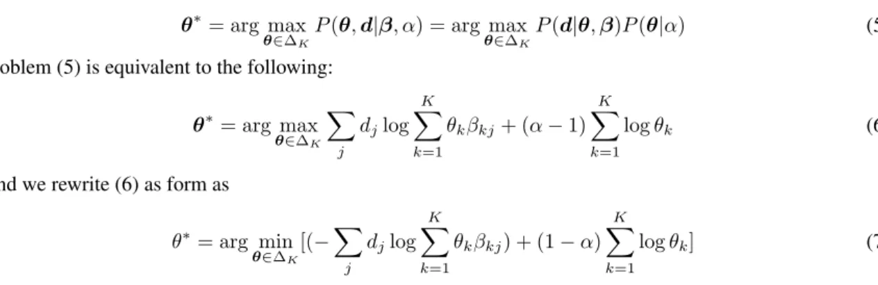
We consider the MAP estimation of topic mixture for a given documentd: θ∗= arg max
θ∈∆K
P(θ,d|β, α) = arg max
θ∈∆K
P(d|θ,β)P(θ|α) (5)
Problem (5) is equivalent to the following: θ∗= arg max
θ∈∆K
X
j
djlog K
X
k=1
θkβkj+ (α−1) K
X
k=1
logθk (6)
And we rewrite (6) as form as θ∗= arg min
θ∈∆K[(−
X
j
djlog K
X
k=1
θkβkj) + (1−α) K
X
k=1
logθk] (7)
We find out that (7) is a non-convex optimization problem whenα <1. This optimization problem is usually non-convex and NP-hard in practice [27]. We denote
g(θ) :=−X
j
djlog K
X
k=1
θkβkj, h(θ) := (1−α) K
X
k=1
logθk
then the objective functionf(θ) =P
jdjlog
PK
k=1θkβkj+ (α−1)
PK
k=1logθk=g(θ) +h(θ). We see that
problem (7) is one case of (2), then we can use GS-OPT algorithm to solve problem (6).
Figure 1. Latent dichlet allocation model
We have seen many attractive properties of GS-OPT that other methods do not have. We further show the simplicity of using GS-OPT for designing fast learning algorithms for topic models. More specifically, based on two learning algorithms with LDA which are ML-OPE and Online-OPE [17], we design two algo-rithms: ML-GSOPT which enables us to learn LDA from either large corpora or data streams, Online-GSOPT which learns LDA from large corpora in an online fashion. These algorithms employ GS-OPT to do MAP in-ference for individual documents, and the online scheme or streaming scheme to infer global variables (topics). Details of ML-GSOPT and Online-GSOPT are presented in Algorithm 2 and Algorithm 3.
Algorithm 2ML-GSOPT for learning LDA from massive/streaming data Input: data sequenceK, α, τ >0, κ∈(0.5,1]
Output:β
1: Initializeβ0randomly in∆V
2: fort= 1,2, . . .∞do
3: Pick a setCtof documents
4: Do inference by GS-OPT for eachd∈ Ctto getθd, givenβt−1
5: Compute intermediate topicβˆtasβˆt kj∝
P
d∈Ctdjθdk
6: Set step-size:ρt= (t+τ)−κ
7: Update topics:βt:= (1−ρt)βt−1+ρtβˆ t
Algorithm 3Online-GSOPT for learning LDA from massive data Input: Training dataCwithDdocuments,K, α, η, τ >0, κ∈(0.5,1]
Output:λ
1: Initializeλ0randomly
2: fort= 1,2, . . .∞do
3: Sample a setCtconsisting ofSdocuments,
4: Use GS-OPT to do posterior inference for each documentd∈ Ct, given the global variableβt−1∝λt−1
in the last step, to get topic mixtureθd. Then, computeφdasφdjk∝θdkβkj
5: For each k ∈ {1,2, . . . , K}, form an intermediate global variable λˆk for Ct by λˆkj = η + D
S
P
d∈Ctdjφdjk
6: Update the global variable byλt:= (1−ρt)λt−1+ρtλˆwhereρt= (t+τ)−κ
7: end for
4. EMPIRICAL EVALUATION
This section is devoted to investigating practical behaviors of GS-OPT, and how useful it is when GS-OPT is employed to design two new algorithms for learning topic models at large scales. To this end, we take the following methods, data-sets, and performance measures into investigation.
4.1. Datasets:
We used the two large corpora: PubMed dataset consists of 330,000 articles from the PubMed central and New York Times dataset consists of 300,000 news. The data sets were taken from http://archive.ics.uci.edu/ml/datasets. For each data set, we use 10,000 documents for the test set.
4.2. Parameter settings:
To compare our methods with another ones, almost of free parameters are the same as in [17]. a. Model parameters: The number of topicsK= 100, the hyper-parametersα= K1 and the topic Dirichlet
parameterη= K1. These parameters are commonly used in topic models. b. Inference parameters: The number of iterations is chosen asT = 50.
c. Learning parameters:κ= 0.9,τ= 1adapted best for existing inference methods.
We do many experiments with two scenarios: (1) Choosing Bernoulli parameterp∈ {0.30,0.35, . . . ,
0.65,0.70}with mini-batch size|Ct|= 25,000; (2) Choosing the Bernoulli parameterp∈ {0.1,0.2, . . . ,0.9}
with the mini-batch size|Ct|= 5,000. We do experiments with GS-OPT by choosing the linear combination
parameterν = 0.3on New York Times andν = 0.1on PubMed. We also can do much more experiments to examine the effect of the parameterν ∈(0,1)in GS-OPT.
4.3. Performance measures:
We usedLog Predictive Probability(LPP) andNormalized Pointwise Mutual Information(NPMI) to evaluate the learning methods. NPMI [28] evaluates semantics quality of an individual topic. From extensive experiments, [28] found that NPMI agrees well with human evaluation on the interpretability of topic models. Predictive probability [26] measures the predictability and generalization of a model to new data.
4.4. Evaluation results: 4.4.1. Inference methods:
Variational Bayes (VB) [22], Collapsed variational Bayes (CVB, CVB0) [24], Collapsed Gibbs sam-pling (CGS) [26], OPE [17], and GS-OPT. CVB0 and CGS have been observing to work best by several previous studies [24, 26]. Therefore, they can be considered as the state-of-the-art inference methods.
4.4.2. Large-scale learning methods:
ML-GSOPT, GSOPT, ML-OPE, OPE [17], CGS [26], CVB [24], Online-VB [29].
To avoid randomness, the learning methods for each dataset are run five times and reported their average results. By changing of variables and bound functions, we obtain GS-OPT which is more effec-tive than OPE. GS-OPT has parameterν ∈ (0,1)when constructing a linear combinationFtofUtandLt,
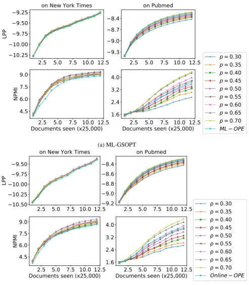
then experimental results of GS-OPT is bad or good depending on howν is chosen. We do some exper-iments for learning LDA with GS-OPT algorithm on two data-sets via choosing Bernoulli parameterp ∈ {0.30,0.35, . . . ,0.65,0.70}with mini-batch size|Ct|= 25,000. [17] shows that OPE is better than previous
methods. Thus, we compare our method with OPE via LPP and NPMI measures and on two datasets. Details of our experimental results on this case are shown in Figure 2.
2.5 5.0 7.5 10.0 12.5 −10.25 −10.00 −9.75 −9.50 −9.25 LP P
on
New Y rk Times
2.5 5.0 7.5 10.0 12.5
−9.3
−9.0
−8.7
−8.4
n Pubmed
2.5 5.0 7.5 10.0 12.5
D cuments seen (x25,000)
4.5
6.0
7.5
9.0
NP
MI
2.5 5.0 7.5 10.0 12.5
D cuments seen (x25,000)
1.6
2.4
3.2
4.0
p=0.30
p=0.35
p=0.40
p=0.45
p=0.50
p=0.55
p=0.60
p=0.65
p=0.70
ML−
OPE(a) ML-GSOPT
2.5 5.0 7.5 10.0 12.5 −10.50 −10.25 −10.00 −9.75 −9.50 LP P
on
New Y rk Times
2.5 5.0 7.5 10.0 12.5
−9.2
−9.0
−8.8
−8.6
−8.4
n Pubmed
2.5 5.0 7.5 10.0 12.5
D cuments seen (x25,000)
4.5
6.0
7.5
9.0
NP
MI
2.5 5.0 7.5 10.0 12.5
D cuments seen (x25,000)
1.6
2.4
3.2
4.0
p=0.30
p=0.35
p=0.40
p=0.45
p=0.50
p=0.55
p=0.60
p=0.65
p=0.70
Online−
OPE(b) Online-GSOPT
Figure 2. Results of GS-OPT with different value ofpwith mini-batch size|Ct|= 25,000. Higher is better,
(a) ML-GSOPT, (b) Online-GSOPT
Via our experiments, we find out that using Bernoulli distribution and two bounds of the objective function in GS-OPT can give results better than OPE. We also see that GS-OPT depends on Bernoulli pa-rameterpchosen. We have made further experiments by dividing the data into smaller mini-batches such as |Ct|= 5,000and choosing the Bernoulli parameterpmore extensive, such asp∈ {0.1,0.2, . . . ,0.8,0.9}, and
parameterν= 0.3on New York Times andν = 0.1on Pubmed dataset. Details of our experimental results on this case are shown in Figure 3.
We find out that GS-OPT gives the different results which depend on Bernoulli parameter pand parameterν chosen. We also find out that using mini-batch size|Ct|= 5,000is better than using mini-batch
size|Ct|= 25,000. It means LPP and NPMI in case of mini-batch size|Ct|= 5,000are higher than in case
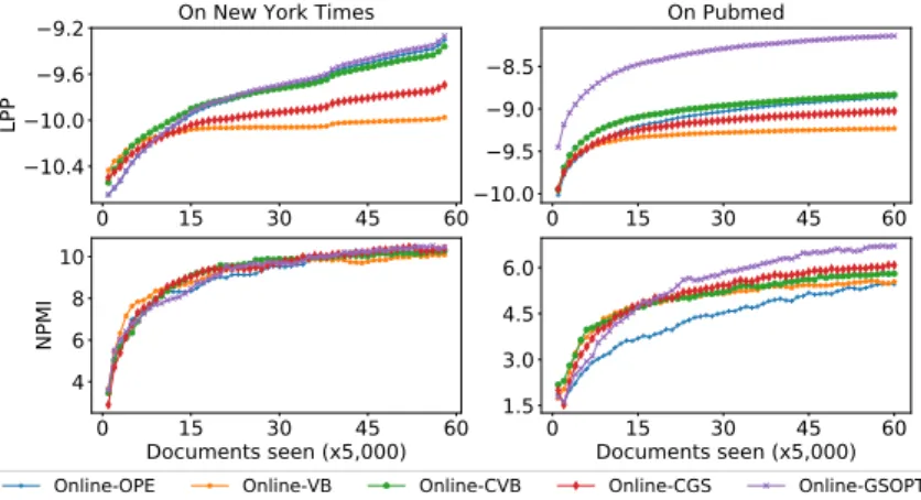
of|Ct| = 25,000. In addition, we find out that Online-GSOPT is better than Online-VB, Online-CVB and
Online-CGS on two datasets with LPP and NPMI measures. Details of these results are shown in Figure 4. This explains the contribution of the prior/likelihood of solving the inference problem.
0 15 30 45 60 −10.2 −9.9 −9.6 −9.3 LP P
on
New Y rk Times
0
15
30
45
60
−9.6
−9.2
−8.8
−8.4
−8.0
n Pubmed
0
15
30
45
60
D cuments seen (x5,000)
4.5
6.0
7.5
9.0
NP
MI
0
15
30
45
60
D cuments seen (x5,000)
1.5
3.0
4.5
6.0
p=0.1
p
=0.2
p=0.3
p=0.4
p=0.6
p=0.7
p=0.8
p=0.9
(a) ML-GSOPT0 15 30 45 60
−10.4 −10.0 −9.6
LP
P
on
New Y rk Times
0
15
30
45
60
−9.3
−9.0
−8.7
−8.4
−8.1
n Pubmed
0
15
30
45
60
D cuments seen (x5,000)
4
6
8
10
NP
MI
0
15
30
45
60
D cuments seen (x5,000)
1.5
3.0
4.5
6.0
p=0.1
p
=0.2
p=0.3
p=0.4
p=0.6
p=0.7
p=0.8
p=0.9
(b) Online-GSOPTFigure 3. Results of GS-OPT with different value ofpwith mini-batch size|Ct|= 5,000. Higher is better,
(a) ML-GSOPT, (b) Online-GSOPT
0 15 30 45 60
−10.4 .10.0 .9.6 .9.2 LP P
On New York Times
0 15 30 45 60
.10.0.9.5
.9.0 .8.5
On Pubme
0 15 30 45 60
Documents seen (x5,000)
4 6 8 10 N PM I
Online-OPE Online-VB Online-CVB Online-CGS Online-GSOPT
0 15 30 45 60
Documents seen (x5,000)
1.5 3.0 4.5 6.0
Figure 4. Performance of different learning methods as seeing more documents. Higher is better. Online-GSOPT is better than Online-OPE, Online-VB, Online-CVB and Online-CGS. We choose mini-batch
5. CONCLUSION
In this paper, we propose GS-OPT, a new algorithm solving efficiently the non-convex optimization problems. Using Bernoulli distribution and stochastic approximations, we provide the GSOPT algorithm to deal well with the posterior inference problem in topic models. The Bernoulli parameterpin GS-OPT is seen as the regularization parameter that helps the model to be more efficient and avoid over-fitting. By exploiting GS-OPT carefully in topic models, we have arrived at two efficient methods for learning LDA from large corpora. As a result, they are good candidates to help us deal with text streams and big data. In addition, GS-OPT is flexible then we can apply it to solve more and more the non-convex problems in machine learning.
ACKNOWLEDGEMENT
This work was supported by the University of Information and Communication Technology (ICTU) under project T2019-07-06.
REFERENCES
[1] L. Bottou, F. E. Curtis, and J. Nocedal, “Optimization methods for large-scale machine learning,”SIAM Review, vol. 60, no. 2, pp. 223-311, 2018.
[2] R. Johnson and T. Zhang, “Accelerating stochastic gradient descent using predictive variance reduction,” Advances in neural information processing systems,pp. 315-323, 2013.
[3] L. Xiao and T. Zhang, “A proximal stochastic gradient method with progressive variance reduction,” SIAM Journal on Optimization,vol. 24, no. 4, pp. 2057-2075, 2014.
[4] A. L. Yuille and A. Rangarajan, “The concave-convex procedure,” textslNeural computation, vol. 15, no. 4, pp. 915- 936, 2003.
[5] A. Blake and A. Zisserman, ”Visual reconstruction,” textslMIT press, 1987.
[6] E. Hazan, K. Y. Levy, and S. Shalev-Shwartz, “On graduated optimization for stochastic non-convex problems,”International conference on machine learning,pp. 1833-1841, 2016.
[7] X. Chen, S. Liu, R. Sun, and M. Hong, “On the convergence of a class of adam-type algorithms for non-convex optimization,”arXiv preprint arXiv:1808.02941,2018.
[8] J. Duchi, E. Hazan, and Y. Singer, “Adaptive subgradient methods for online learning and stochastic optimiza- tion,”Journal of Machine Learning Research,vol. 12, pp. 2121-2159, 2011.
[9] T. Tieleman and G. Hinton, “Lecture 6.5-rmsprop: Divide the gradient by a running average of its recent magni- tude,”COURSERA: Neural networks for machine learning,vol. 4, no. 2, pp. 26-31, 2012. [10] D. P. Kingma and J. L. Ba, “Adam: Amethod for stochastic optimization,” Proc. 3rd Int. Conf. Learn.
Repre- sentations,2014.
[11] M. D. Zeiler, “Adadelta: an adaptive learning rate method,”arXiv preprint arXiv:1212.5701,2012. [12] S. Ghadimi and G. Lan, “Accelerated gradient methods for nonconvex nonlinear and stochastic
programming,” Math. Program.,vol. 156, no. 1-2, pp. 59-99, 2016.
[13] Z. Allen-Zhu, “Natasha 2: Faster non-convex optimization than sgd,”Advances in Neural Information Processing Systems. Curran Associates, Inc.,pp. 2680-2691, 2018.
[14] Z.Allen-ZhuandY.Li, “Neon2: Finding local mini mavia first-orderoracles,” Advances in Neural Information Processing Systems,pp. 3720-3730 2018.
[15] C. J. Hillar and L.-H. Lim, “Most tensor problems are np-hard,” Journal of the ACM (JACM),vol. 60, no. 6, p. 45, 2013.
[16] E. Hazan and S. Kale, “Projection-free online learning,” Proceedings of Annual International Conference on Machine Learning,2012.
[17] K. Than and T. Doan, “Guaranteed inference in topic models,”arXiv preprint arXiv:1512.03308,2015. [18] J. Mairal, “Stochastic majorization-minimization algorithms for large-scale optimization,” Advances in
neural information processing systems,pp. 2283-2291, 2013,.
[19] B. Dai, N. He, H. Dai, and L. Song, “Provable bayesian inference via particle mirror descent,”Artificial Intelligence and Statistics,pp. 985-994, 2016.
[20] U. Simsekli, R. Badeau, T. Cemgil, and G. Richard, “Stochastic quasi-newton langevin monte carlo,” Interna- tional Conference on Machine Learning (ICML),2016.
optimization,” Proceedings of 54th Annual Allerton Conference on Communication, Control, and Computing,pp. 1244-1251, 2016,
[22] D. M. Blei, A. Y. Ng, and M. I. Jordan, “Latent dirichlet allocation,” Journal of machine Learning research,vol. 3, pp. 993-1022, 2003.
[23] Y. W. Teh, K. Kurihara, and M. Welling, “Collapsed variational inference for hdp,” Proceedings of Advances in Neural Information Processing Systems,pp. 1481-1488, 2007.
[24] A. Asuncion, M. Welling, P. Smyth, and Y. W. Teh, “On smoothing and inference for topic models,” Proceed- ings of the Twenty-Fifth Conference on Uncertainty in Artificial Intelligence. AUAI Press, pp. 27-34, 2009.
[25] T. L. Griffiths and M. Steyvers, “Finding scientific topics,”Proceedings of the National academy of Sci-ences,vol. 101. National Acad Sciences, pp. 5228-5235, 2004.
[26] M. Hoffman, D. M. Blei, and D. M. Mimno, “Sparse stochastic inference for latent dirichlet allocation,” Proceedings of the 29th International Conference on Machine Learning (ICML-12). ACM,pp. 1599-1606, 2012.
[27] D. Sontag and D. Roy, “Complexity of inference in latent dirichlet allocation,”Proceedings of Advances in Neural Information Processing System,2011.
[28] J. H. Lau, D. Newman, and T. Baldwin, “Machine reading tea leaves: Automatically evaluating topic coherence and topic model quality,” Proceedings of the 14th Conference of the European Chapter of the Association for Computational Linguistics,pp. 530-539, 2014.
[29] M. D. Hoffman, D. M. Blei, C. Wang, and J. W. Paisley, “Stochastic variational inference,”Journal of Machine Learning Research,vol. 14, no. 1, pp. 1303-1347, 2013.