Sharif University of Technology
Scientia IranicaTransactions C: Chemistry and Chemical Engineering www.scientiairanica.com
Optimal operation of a divided-wall column with local
operating condition changes
A. Arjomand and M.A. Fanaei
Department of Chemical Engineering, Ferdowsi University of Mashhad, Mashhad, Iran. Received 25 August 2014; received in revised form 4 July 2015; accepted 17 August 2015
KEYWORDS Optimal operation; Divided-wall column; Plantwide control; Self-optimizing control;
Takagi-Sugeno fuzzy inference system.
Abstract.The aim of this paper is optimal operation of a Divided-Wall Column (DWC) based on Self-Optimizing Control (SOC). By now, the proposed SOC methods have been based on linearization of the process. The novelty of this paper is to overcome this shortcoming of the local optimality of SOC. Theoretically, changes in optimal sensitivity matrix from nominal design, due to changes in the operating condition, make SOC deviate from steady state optimality. These deviations from optimal operation, in already available SOC structures, have to be counteracted by the optimization layer in the control structure hierarchy which involves solving a large nonlinear optimization problem online. The proposed method in this paper solves this problem by modeling the optimal sensitivity matrix with Takagi-Sugeno fuzzy inference. This fuzzy inference system is tuned oine. The proposed method is dynamically validated and compared with conventional SOC. The results showed that the conventional SOC had a high value of loss and deviated from the optimal operation. However, in the same operating condition, the proposed method with the aid of Takagi-Sugeno fuzzy inference system, which involves online calculation of the weighted average of some linear functions, imposed a small loss, made DWC track an optimal trajectory, and removed the need for solving the large nonlinear optimization problem online.
© 2015 Sharif University of Technology. All rights reserved.
1. Introduction
Optimal operation of the plants has a growing demand nowadays. The price of energy, environmental regula-tions and competiregula-tions make the process plants operate as close as possible to the optimal operation. Generally, steady state operation takes the largest amount of operating cost. So, noticeable economic benets can be achieved by optimal steady state operation [1]. A control structure that yields nice transient responses and tight control by keeping the selected controlled variables at their specied setpoints may be useless if it provides a non-economical steady state performance.
*. Corresponding author. Tel.: +98 5138805061; Fax: +98 5138816840
E-mail address: [email protected] (M.A. Fanaei)
Moreover, operation at a pre-designed nominally op-timal point may not necessarily be actually opop-timal, due to real-time disturbances, measurement errors, and uncertainties.
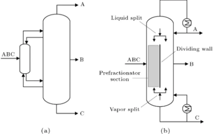
On the other hand, process intensication makes new processes with more complex multivariable sys-tems which require a suitable control structure for the expected operating condition. The Divided-Wall Column (DWC) is an important example of process intensication [2]. It is an implementation of the topology of fully thermally coupled Petlyuk column [3], as shown in Figure 1. DWC can reduce up to 30% in the capital invested and up to 40% in the energy costs [4]. Reduced mixing loss via reduction in remixing eect, which happens usually in conventional distillation trains, can make considerable savings [5, 6]. The value of saving is dependent on feed composition,
Figure 1. Separation of ternary mixture with (a) Petlyuk conguration, and (b) divided-wall column.
relative volatility, and product purity specication and can be higher in the case of separation of mixtures with more components [7]. In this way, DWC overcomes the usual problem of trade-o between the operation cost and the investment costs when reducing operating cost at the expense of higher investment costs [8]. Also, DWC reduces space requirements by 40% compared to the conventional distillation columns [9].
However, in spite of all these clear advantages, the practical use of DWC at industrial scale is still limited to only a few companies [10], because DWCs have the coupling eect of various phenomena such as mass and energy ows of vapor and liquid which meet above and below the wall and transfer heat across the dividing wall [11]. It makes DWC a comparatively complex multivariable system [12], and understanding its operability and controllability is still a growing matter [4]. Moreover, real-time disturbances in a DWC with xed vapor and liquid split fraction may move the system to a region where the solution to the optimization problem (optimum operation) is located on a sharp peak (sharp optimum) and the system may be unstable or at least unable to obtain reasonable energy saving [13]. Thus, it seems dicult to achieve the potential energy savings in a DWC without a good control strategy compared to conventional approaches. Control structure design generally classies problems into two classes. In the rst class, all the optimization degrees of freedom are used to satisfy active constraints for all expected disturbances at the optimal solution, while in the second class, which is the focus of this work, one or more optimization degrees of freedom are unconstrained. In the second type of problem, choosing the Controlled Variable (CV) is a very important step in the control structure design in order to obtain optimal operation in practice. Traditionally, controlled variables have been selected based on intuition and process knowledge. Skogestad [14] presented a method for selecting Self-Optimizing Controlled (SOC) variable in the form of some function of the measured variables
in such a way that keeps this controlled variable constant, or slowly varying, making the process operate close to economically optimal steady state operation in the presence of disturbances and implementation errors.
In other words, SOC structure design aims to remove or at least decrease the need for solving a nonlinear optimization problem online by converting the optimization problem into a feedback problem. By now, SOC design has been based on linearization of the process model around the nominal operating point. The rst approach for SOC design was the maximum gain rule [15] with local consideration of process model. Halvorsen et al. [16] presented the exact local method with the worst-case loss based on the linear model around the nominal operating point and quadratic expansion of the objective function which leads to nonlinear optimization problem. This work was reformulated as a quadratic optimization problem with linear constraints by Alstad et al. [17] which is easier to solve numerically; also, Yelchuru and Skogestad [18] proposed a simpler and more practical calculation. For local linear combination of measurements, Kariwala et al. [19] proposed another method and minimized average loss for local SOC. Alstad and Skogestad [20] devised null space method wherein combination matrix was located in the left null space of local optimal sensitivity matrix. However, null space method holds its optimality for small deviations from the nominal optimum (small magnitude of the disturbance) and is globally optimum in cases wherein the optimal sensitivity matrix, F, is not dependent on the operating point (disturbances) or, in other words, for a system with a quadratic cost objective function and linear model equations [20].
So, in a complex multivariable process with varying operating conditions, the local consideration of process makes SOC design deviate from nominal optimal steady-state operation. This could be coun-teracted with solving a nonlinear optimization online in optimization layer which is located above the SOC in control structure hierarchy. But, this causes the main role of SOC in removing or decreasing the need for solving large nonlinear optimization problem online become violated. Moreover, this deviation from local optimal design becomes more severe in a more complex multivariable system such as DWC.
With the local consideration of DWC, Arjomand and Fanaei [21] designed a SOC structure with the maximum gain rule [15] which was based on the con-ventional individual measurement. In the other work, Arjomand and Fanaei [1] developed a SOC structure with the exact local method [16] and it was shown that it was possible to have better self-optimizing properties by controlling linear combinations of mea-surements than by controlling conventional individual
measurements in control structure of a DWC. However, the proposed SOC structure of Arjomand and Fanaei [1] for DWC has the weakness of local optimality problem. The current work presents a novel method for solving the shortcoming of local optimality of SOC through modelling F with Takagi-Sugeno (T-S) fuzzy inference system in the null space method [20]. In other words, our main concern in this paper is to extend the self-optimizing property of the control structure for a DWC to large variation in operating condition where optimal sensitivity matrix changes from nominal design.
The T-S fuzzy model can represent nonlinear system by decomposing the whole input space into several fuzzy sets and representing each output space with a linear equation. Such a model is capable of ap-proximating a wide class of nonlinear systems. For the reason that it employs linear model in the consequent part, conventional linear system theory can be applied for system analysis and synthesis accordingly. And hence, the T-S fuzzy models are becoming powerful engineering tools for modelling and control of complex systems.
This paper is organized as follows. The next section describes mathematical formulation of null space method and the basics of T-S fuzzy inference system. Section 3 will review the general structure of a plantwide multilayer control structure and will present the proposed multilayer control structure with fuzzy system. Section 4 will design control structure for the studied DWC which is followed by results and discussions in Section 5 and, nally, conclusion in Section 6.
2. Preliminaries
2.1. Mathematical formulation
To quantify \acceptable operation" or close to optimal steady state operation, a scalar cost function J is considered which should be minimized for optimal operation. The (economic) cost mainly depends on the steady-state behavior, which is a good assumption for most continuous plants in the process industry.
Generally, the original independent variable u0
is divided into the constrained variable u0 which is
used to satisfy active constraints f0(x; u; d) = 0 and
the remaining unconstrained variable u(u0= fu0; ug).
It is assumed that any optimally \active constraint" has been implemented so that u0 includes only the
re-maining unconstrained steady-state degrees of freedom. Finally, the objective is to achieve optimal steady-state operation, where the degrees of freedom u are selected such that the scalar cost function J(u; d) is minimized in the \reduced space" optimization problem with respect to the unconstraint degrees of freedom for any expected disturbance d by solving the following
problem. min
x;uJ(x; u; d);
Subject to: f(x; u; d) = 0; g(x; u; d) 0;
x 2 Rnx; u 2 Rnu; d 2 Rnd; (1)
where x, u, and d are the states, inputs, and distur-bances, respectively; f is the set of equality constraints corresponding to the model equation; g is the set of inequality constraints that limits the operation. The objective of SOC is to nd an optimal measurement combination:
c = Hy; (2)
such that a constant setpoint, cs, policy, in which u is
adjusted to keep c constant on cs, yields near optimal
operation in accordance with Eq. (1) where:
cs= Hyopt: (3)
To quantify the dierence between alternative choices of c, the loss is dened as the dierence between the actual cost and the optimal cost:
L = J(u; d) J(uopt; d); (4)
where for a given d, solving Eq. (1) gives uopt(d). In
the reduced space after implementing active constraints and elimination of the states using model equation:
y = fy(u; d); (5)
and in a local linearized model around nominal oper-ating point (*), the measured variables are:
y = Gyu Gy
dd; (6)
where Gy = @fy
@u
T
and Gy d =
@fy
@d
T
. The controlled variable c is the selected function of y:
c = h(y); (7)
where the function h is free to choose. By substituting Eq. (5) into Eq. (7) the following equation is obtained: c = h [fy(u; d)] = fc(u; d): (8)
And the linearized model in the reduced space is expressed as follows:
c = Gu Gdd; (9)
where G =@fc
@u
T
and Gd =
@fc
@d
T .
2.2. Null space
The null space method [20] deals with the optimal selection of linear measurement combinations as the controlled variables, c = Hy, for quadratic approxima-tion of Eq. (1) with the second-order Taylor expansion of the cost function J(u; d):
min
u d
TJ
uu Jud
Jdu Jdd
u D
; (10)
where Juu= @@u2J2, Jud= JTdu= @ 2J
@u@d, and Jdd=@
2J
@d2.
Considering that nuis the number of independent
unconstrained free variable u, nd is the number of
independent disturbance d, and ny is the number of
measurement y. If ny nu+nd, it is possible with the
null space method [20] to select combination matrix H in the left null space of F, or:
H = null(FT); (11)
such that its optimal value is independent of d where F is optimal sensitivity matrix evaluated with the following denition:
F =@y@doptT : (12) Also F could be calculated from linearized local model [17]:
F = GyJ 1
uuJud Gyd
: (13)
With this choice for H, xing c (at its nominal optimal value) will lead to zero loss as long as F does not change [20].
The optimal sensitivity matrix, F, may be com-puted from Eq. (13). However, in practice, it is usually easier to obtain F, numerically. In other words, for practical use, it is more reliable to obtain F, numerically, from its denition in Eq. (12), instead of deriving an analytical expression from Eq. (13) [18]. Moreover, providing analytical expression of F for the entire operation space in a complex of nonlinear chemical plants from explicit representation of the model equations is even a more dicult problem to be solved, but is readily to be solved numerically through fuzzy modelling.
2.3. Takagi-Sugeno fuzzy inference system Fuzzy sets are characterized by membership functions or degree of truth of v in A that map R to the membership space:
A = f(v; (v)) jv 2 Rg : (14) The membership function is described by an arbitrary curve suitable from the point of view of simplicity, con-venience, speed, and eciency. When the membership
space contains only 0 and 1, A is nonfuzzy and is a characteristic function of non-fuzzy set. The range of the membership functions is a subset of the nonnegative real numbers. In this paper, Gaussian membership functions is regarded as follows:
(v) = exp
1 2
v
; (15)
where is the center of the membership function and is a constant related to the spread of membership function.
Structure of a Takagi-Sugeno fuzzy inference sys-tem is shown in Figure 2. It is a model that maps characteristics of input data to input membership functions, input membership functions to rules, rules to output crisp functions, and output crisp functions to a single-valued output [22]. Generally, the process of formulating the mapping from a given input to an output using fuzzy logic is called the fuzzy inference.
In T-S fuzzy systems, the relationships between variables are represented by the means of fuzzy if-then rules as follows:
Rulei: If v1is A1i and v2 is A2i ::: vn is Ani
Then zi= i(v1; v2; :::; vn); (16)
where v = [v1; v2; :::; vn]T is the vector of input
variables, Aji(1 j n) represents fuzzy set, zi is
the output of rule i, and i is a crisp function of rule i.
In the rst-order sugeno model, a linear combination of input variables is considered as the consequent crisp function as follows:
i(v1; v2; :::; vn)=b0i + bi1v1+ b2iv2+ ::: + bnivn: (17)
As such, each rule can be considered as a local linear model that will fuse with others to produce an overall nonlinear output z. Given the input vector v = [v1; v2; :::; vn]T, the model output z is the weighted
average of the individual rule outputs zi(1 i Nr)
according to the following formula:
z = PNr
i=1wizi
PNr
i=1wi
; (18)
where Nr is the number of rules, and wi is the ring
strength of rule i calculated as follows:
wi= nj=1ji(vj); (19)
where denotes the fuzzy MIN operator and ji is the membership function corresponding to fuzzy set Aji. 2.3.1. Parameter tuning
One of the most successful fuzzy system identication methodologies within the realm of soft computing is genetic fuzzy system where Genetic Algorithm (GA) is considered to learn the components of a fuzzy rule-based system [23]. A genetic fuzzy system is basically a fuzzy system augmented by a learning process based on a GA and has been coined by a hybridization between GA and fuzzy rule-based system [24]. Genetic learn-ing processes can cover dierent levels of complexity according to the structural changes produced by the algorithm, from parameter optimization to the highest level of complexity of learning the rule set of a rule-based system [25]. Owing to the fact that T-S type fuzzy system has a linear consequent part, using the least square with GA has also combined the advantages of both algorithms to enhance its search capability; also, the optima can be located more quickly [26].
The T-S fuzzy system parameters are automati-cally tuned from numerical information (input-output data sets from nonlinear model). An input variable is changed instantly and, at the same time, the behavior of the output variables is collected. Then, the same procedure is performed for the other input variables and nally a data set for identication of the fuzzy models is obtained by oine calculation in nonlinear model. Subsequently, the identication data set is divided into training data set and test data set with random method [22]. The training data set is used for tuning model parameters and these models are then validated through the test data.
In brief, the GA starts with a community of chro-mosomes known as the initial population. In contrast with classical algorithm which generates a single point at each iteration, GA generates a population of points at each iteration. Then, the chromosomes are passed to the objective function. As the aim is to minimize the error between the output of fuzzy model and output data, the Mean of Squared Error (MSE) is used as evaluation function.
Among the chromosomes in the population, some of them will be arbitrarily selected. This selection component in the GA guides the algorithm to the solution. One approach used in this work, to guide the selection procedure, is stochastic uniform selection function. This reproduction population will then be mated through crossover component. Crossover is the process of creating one or more osprings from the current population. In this work, arithmetic crossover is used. The last component of GA is mutation. Mutation rules apply random changes to individual to form the next generation. This process is performed to prevent the algorithm from sticking at local minimum by introducing traits not existing in the original population. Gaussian mutation is applied in this work. The so called selection, crossover, and mutation are the three main types of rules at each step to create the next generation from current population. In this work, we use MATLAB software to implement genetic algorithm. For more information about genetic algorithm one can refer to MATLAB software user's guide.
Also, the coecients of the crisp linear functions are constructed with least square estimation method and are dependent on the values of the membership functions in the antecedent part. So, this is quite dierent from linear model identication wherein the coecients of the model can be directly calculated from the input variable values. Therefore, in using the least square method, at rst, the equations of the output are rearranged to comply with the least square equation as in Appendix A, and the coecients of the linear equations of fuzzy model can be identied indirectly from the values of input variables and the membership for each rule. The parameter tuning algorithm can be summarized as follows:
1. Generate random initial population;
2. Evaluate objective function for every chromosome.
(2-i) Use least square method to dene the pa-rameter of linear equations by the desired membership functions parameters;
(2-ii) Calculate MSE for every chromosome.
3. Perform selection, crossover, and mutation opera-tion to produce new populaopera-tion;
Figure 3. General multilayer control structure [27].
generations to get the best individual which will represent the best fuzzy model.
3. Multilayer control structure
In a complex real chemical plant, a straightforward task of designing and implementing a single centralized control unit is too dicult and, in many cases of complex multivariable processes, is just impossible. Hierarchical multilayer control structure is a solution in such complex situations [27]. The main idea is to decompose the original control task into a sequence of simpler and hierarchically structured subtasks that are handled by dedicated control layers, as shown in Figure 3.
The direct control layer is responsible for safety of dynamic processes in the plant. The main feature of all direct (basic) controllers is direct access to the controlled process (process manipulated variables are outputs of the direct controllers). Algorithms of direct control should be robust and relatively easy, in structure and design method, that is why classic Proportional-Integral-Derivative (PID) algorithms are still dominant. However, rapid development of com-puter technology made it now possible to apply Model Predictive Control (MPC) also for direct control, when improved control performance is required and cannot be achieved with PIDs [28].
The setpoint control layer keeps high quality of operation. This layer usually does not fully separate the direct control layer from the optimization layer, and some of the setpoints for basic controllers can be assigned and directly transmitted from the optimiza-tion layer, as can be seen in Figure 3.
The real process operation is always under uncer-tainty. A process plant is not isolated from its envi-ronment and it undergoes controlled and uncontrolled
external inuences. One source of the uncertainty is the behavior of disturbances (uncontrolled process inputs). Usually, some parts of these variables are measured or estimated and some others are not. Optimal values of the setpoints are dependent on these disturbance values and vary when their values vary. The optimal operating point is calculated for current values of disturbances, and recalculated after signicant changes in these values [27].
Uncertainty makes a single optimization layer usually lead to solutions being only suboptimal set-points for the real process, with the degree of subop-timality dependent on the level of uncertainty. There-fore, a setpoint optimization at the optimization layer is dened to obtain optimal setpoints of feedback controllers, for current measurements or estimates of the disturbances taken into account in the model which are additionally marked with dashed lines in Figure 3. It performs economic optimization related to the controlled process, which is usually a part of a larger complex plant. The goal is to calculate the process optimal operating point or optimal operating trajectory, i.e. optimal steady-state values of setpoints for current values of disturbance measurements or estimates to be applied for feedback controllers of directly subordinate layers (regulatory layer). So, with decomposing the original centralized control task into a sequence of simpler and hierarchically structured subtasks and assigning a specic task to each layer, which includes feedback information, it copes with the various uncertainties.
3.1. Fuzzy system in multilayer control structure
If a disturbance moves the process far from the nom-inal point, the local model approximation used for the calculation of self-optimizing CVs by linearization of the nominal operating point and assumption of the quadratic cost function (or approximation of the objective function by the second order Taylor series) may be poor. Therefore, the self-optimizing control task in providing near optimal operation in the case of disturbances which move the process away from the nominal operating point becomes poor. This is usually counteracted by reoptimization of the process with an optimization layer which involves solving a nonlinear optimization online.
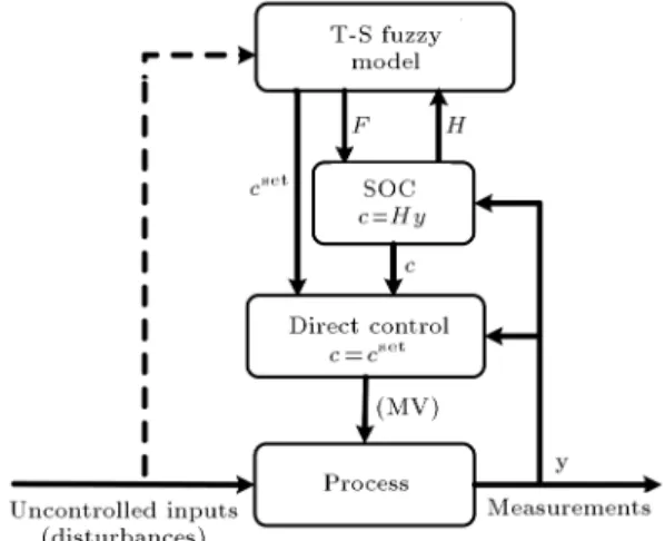
Using fuzzy model makes control structure meet changes in operating condition. Figure 4 shows the proposed control structure with fuzzy inference system. In the proposed algorithm, optimal sensitivity matrix is calculated through the T-S fuzzy inference system. The null space receives optimal sensitivity matrix from T-S fuzzy model as well as the selected measurement from plant. The self-optimizing controlled variable is controlled through a controller, which is generally a
Figure 4. Multilayer control structure with T-S fuzzy inference system.
proportional-integral controller. The setpoint for this controller is calculated with Eq. (3) where yopt is, in
accordance with the dening Eq. (12), as follows:
yopt=Z Fdd: (20)
4. Design of control structure
Here, a systematic procedure for control structure design for complete process plants (plantwide control) by Skogestad [29] is followed.
4.1. Process details
In this paper, separation of 1 kmol/s mixture of benzene/toluene/o-xylene with the relative volatility of 7.1/2.2/1 is studied. The design of DWC in this paper is based on the results of optimal steady-state design of Ling and Luyben [30]. Feed enters the DWC at the temperature of 358K and with the concentration of 30/30/40 mol% B/T/X. Physical property package used for this simulation is Chao-Seader in the Aspen simulator. DWC is simulated using two absorbers, single stripper, and a rectier column as [30,31]. There are 24 stages in prefractionation and also in sidestream section, 9 stages in rectier section, and 13 stages in stripper section. Feed enters at stage 12 and sidestream withdraws at stage 44. Product purities are 99 mol%, condenser pressure is 0.37 atm, tray pressure drop is 0.0068 atm, and the reux ratio is 2.85.
4.2. Denition of objective function, degrees of freedom, and optimization
The objective is to minimize reboiler energy consump-tion. With the constant feed ow rate and pressure, there are 7 dynamic degrees of freedom [32]. However there are two liquid level inventories that need to be controlled and since these levels have no steady-state eect, the number of degrees of freedom for steady-state optimization is 5 [33]. Three product purities are
Figure 5. Surface plot for reboiler heat duty as a function of liquid and vapor split fraction.
three active constraints maintained by three freedom degrees. So, two unconstrained degrees of freedom, namely vapor and liquid split fraction, are left to minimize energy. The surface plot in Figure 5 shows that how reboiler heat duty changes with these two unconstrained degrees of freedom. At optimum, vapor and liquid split fraction at the bottom and top of the wall is 0.625 and 0.353, and reboiler heat duty is 35.6 MW.
From practical point of view, it is a more re-alistic case where the vapor split is not a degree of freedom [34] and it does not change later on during the operation [10]. In this paper, we also consider that the vapor split is not a degree of freedom. Therefore, there is one remaining unconstrained degree of freedom. In addition, active constraints (product composition) and also feed composition are considered as important disturbances.
4.3. Identication of measurements and selection of CVs
It is common in distillation column control to use temperature as measurement. In this work, all of the DWC stage temperatures are selected as candidate measurements. So, it has 70 individual candidate measurements (stages 1 to 24 in prefractionator, 25 to 33 in rectier, 34 to 57 in sidestream, and 58 to 70 in stripper section).
There are 4 disturbances (nd = 4) and one
unconstrained degree of freedom (nu = 1). Based on
the null space method in Section 2.2, the minimum number of measurement is ny= 5 (ny nu+ nd). So,
5 stage temperature measurements must be selected among all 70 individual candidate measurements. To select these 5 stage temperatures among all 70 can-didate stage temperatures, the maximum gain rule is used [15]. The maximum gain rule method selects variables with maximum gain of the appropriately scaled steady-state gain matrix Gscl from inputs (u)
to the selected controlled variables (c). It identies candidate controlled variables that satisfy all of the following requirements [14]:
2. Easy to measure and control so that the implemen-tation error is small;
3. Sensitive to changes in the manipulated variables;
4. Independent selected controlled variables (for cases with two or more controlled variables).
The key part of this procedure is scaling of each q-th input and p-th controlled variable. Each q-th candidate input is scaled with Eq. (21). By this scaling, a unit deviation in each input from its optimal value produce the same eect on the cost function [16].
uscl;q = q 1
[Juu]qq
: (21)
The Hessian matrix is calculated with nite dierence and is Juu = 8327. The maximum optimal variation
due to variation in disturbance "p is [16]:
"p=GJuu1Jud Gd(dmax d); (22)
where the Hessian matrix is Jud = [ 995 766
17922 341] and the maximum expected magnitude of disturbance is 10% of nominal value. The scaling factor in Eq. (23) is dened to scale controlled variable such that for each p-th controlled variable, the sum of the magnitude of "pand the implementation error np
become similar [16]:
cscl;p= j"pj + jnpj : (23)
The implementation or measurement errors are taken to be 0.3 degree Celsius. And nally the scaled gain matrix is:
Gscl = Dc1GDu; (24)
where Dc= diagfcscl;pg and Du= diagfuscl;qg are the
diagonal scaling matrices. The rst 5 measurements among all 70 candidate measurements with the largest scaled gain with corresponding scaled gains are shown in Table 1. Therefore, the measurement vector is y = [T1 T14 T15T55 T56]T.
4.4. Design of CV
The sensitivity matrix F is obtained numerically from nonlinear model by perturbing each of the four
distur-Table 1. The rst ve individual measurements with the largest scaled gain.
Rank CV Scaled gain
1 Temperature on tray no. 56 0.979 2 Temperature on tray no. 14 0.915 3 Temperature on tray no. 15 0.783 4 Temperature on tray no. 1 0.762 5 Temperature on tray no. 55 0.575
bances around nominal operating point directly from the dening Eq. (12). The null space method gives the combination matrix H with Eq. (11) and the corresponding CV with Eq. (2) as follows:
c= 454T56 900T14+ 1180T15+T1+ 309T55: (25)
4.5. T-S fuzzy modelling
Optimal sensitivity matrix is modeled through the T-S fuzzy inference system. The fuzzy if-then rules represent the relationships between variables as follows:
Rulei: If d1 is A1i and d2 is A2i and d3is A3i
and d4is A4i Then :
i(k; j) = b0i(k; j) + b1i(k; j)d1+ b2i(k; j)d2
+b3
i(k; j)d3+ b4i(k; j)d4: (26)
The fuzzy domain of input space is equally partitioned with three fuzzy sets to avoid redundant information in the form of similarity between fuzzy sets [35]. Recently, attention has been increasingly paid to improve the transparency and interpretability of fuzzy systems. The transparency and compactness of the fuzzy rule base can even be further improved by methods like rule reduction or rule-base simplication [36]. As there are four disturbances (d1; d2; d3; d4), the inference system
consists of 81 rules (1 i 81) for elements of optimal sensitivity matrix. Optimal sensitivity matrix F has ve rows (1 k 5) for each measurement and four columns (1 j 4) for each disturbance, and i(k; j)
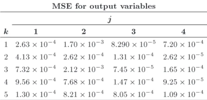
is the local linear representation of the corresponding element, F(k; j), with rule i. The identication data set with 100 elements is divided into training and test data set with 80 and 20 elements, respectively, with random method [22]. The parameters are tuned by tuning algorithm procedure described in Section 2.3.1. The fuzzy models are then validated through the test data and Table 2 demonstrates the validation results of the fuzzy models for the test data set. Small errors in Table 2 show that T-S fuzzy models are close to nonlinear model. Moreover, the performance of the
Table 2. Error quantication for output variables. MSE for output variables
j
k 1 2 3 4
1 2:63 10 4 1:70 10 3 8:290 10 5 7:20 10 4 2 4:13 10 4 2:62 10 4 1:31 10 4 2:62 10 5 3 7:32 10 4 2:12 10 3 7:45 10 5 1:65 10 4 4 9:56 10 4 7:68 10 4 1:47 10 4 9:25 10 5 5 1:30 10 4 8:21 10 4 8:05 10 4 1:09 10 4
Figure 6. The fuzzy domain partitions of the input space.
tuned T-S fuzzy model will be dynamically evaluated in the control structure of DWC. The fuzzy domain of the input space is as shown in Figure 6.
4.6. Dynamic validation
Proportional-Integral (PI) controller is used in the control structure. Pairing of manipulated variables and controlled variables forms a simple multiloop decentral-ized structure (DB/LRSQR) which is used frequently in
the direct control layer of DWC in literatures such as Kiss and Rewagada [4] and Vandiggelen et al. [37]. In this structure, the concentration of benzene in distillate product, the concentration of toluene in side product, and the concentration of xylene in bottom product are controlled with reux ow, side stream ow, and reboiler heat duty, respectively. This control structure is shown in Figure 7. The 5 points on column trays in Figure 7 show the locations of the selected tray temperature measurements which are selected with the maximum gain rule in Section 4.3. A 5-minute dead time is added in all composition loops, and level controllers are proportional only with the gain value of 2. PI controllers are tuned with SIMC method [38] and the controller parameters are shown in Table 3.
5. Results and discussions
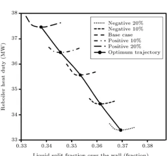
DWC has a complex multivariable system. Figure 8 shows the eect of changes in liquid split fraction over the wall on reboiler heat duty in dierent values of feed toluene concentration. It also shows that how the minimum value of reboiler heat duty changes with dierent values of toluene concentration in the feed
Figure 7. Control structure conguration for divided-wall column.
(disturbance). A negative 20% change means the toluene is changed from 30 mol% to 24 mol% while the other two feed compositions are changed and kept in the same ratio of 30/40, as base case, to make total add of 100 mol%. Therefore, a simple open loop
Table 3. Controller tuning parameter. Controller Controlled Manipulated
Closed loop kc I
variables variable time constant, (%/%) (min) c (min)
CC1 xD LR 275 1.7 150
CC2 xS S 130 1.5 100
CC3 xB QR 124 2.4 120
SOC controller Self-optimize control Liquid split fraction 412 1.9 100
Figure 8. Eect of changes in liquid split fraction over the wall on reboiler heat duty in dierent feed toluene concentration.
feedforward control will lead to suboptimal solution, if it does not lead to an infeasible operation. Since controlling reboiler heat duty in a feedforward fashion on its optima may impose infeasible operation, the reboiler heat duty implemented by control structure goes lower than real optimum reboiler heat duty. So, a more advanced control structure is necessary to provide a stable as well as optimal operation.
To compare the proposed method in this paper with the conventional null space method, two methods are studied in rejecting the same disturbance trajectory entered into the plant, according to Figure 9.
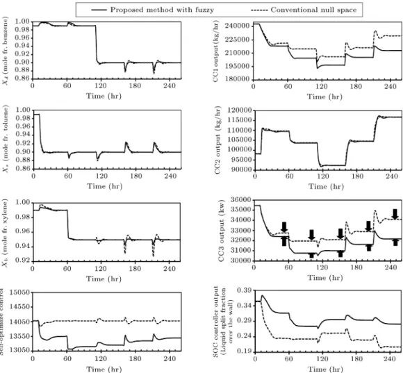
Figure 10 compares dynamic responses of the fuzzy based method, which is proposed in this paper,
Figure 9. Disturbance trajectory.
and conventional null space method. It shows that both methods with the help of low-complexity simple PI controller stabilize the plant, reject the eect of disturbances, and make DWC to produce the prod-uct with desired specications. Here \stabilization" means that the process does not drift too far away from the designed operational point when there are disturbances [29]. Bold ashes in Figure 10 (in CC3 controller output graph) show that the proposed control structure with fuzzy inference system has a lower steady-state reboiler heat duty than that of the conventional control structure. So, it results that the conventional control structure, which is based on local approximation of the nominal operating point, deviates from near optimal operating condition, in comparison with the proposed method based on fuzzy model, and it needs optimization online.
Table 4 shows the loss from the nonlinear model, with Eq. (4), for the conventional null space method. By comparing the values of Table 4 with those of Table 5, it is clear that the proposed method with
Table 4. Nonlinear loss imposed by the conventional null space.
Disturbance Loss (KW) Loss (percent of
nominal value) d1 : decreased toluene mole fraction in S to 0.9 457.6 1.2 d2 : decreased xylene mole fraction in B to 0.95 1052.7 2.9 d3: decreased benzene mole fraction in D to 0.9 1112.8 3.1 d4 : increased toluene mole fraction in F to 0.33 1279.9 3.5 d5 : increased toluene mole fraction in F to 0.36 1943.9 5.4
Figure 10. Dynamic responses of the proposed multilayer control structure with fuzzy inference system in comparison with the conventional control structure.
Table 5. Nonlinear loss imposed by the proposed control structure with fuzzy model.
Disturbance Loss (KW) Loss (percent of
nominal value) d1 : decreased toluene mole fraction in S to 0.9 8.2 0.023 d2 : decreased xylene mole fraction in B to 0.95 1.8 0.005 d3 : decreased benzene mole fraction in D to 0.9 4.7 0.013 d4 : increased toluene mole fraction in F to 0.33 4.2 0.012 d5 : increased toluene mole fraction in F to 0.36 7.4 0.020
fuzzy model has reduced the loss to approximately zero, from the practical point of view. This means that fuzzy modelling of optimal sensitivity matrix makes control structure meet changes in operating condition imposed by successive disturbances entered into the plant. To be more precise, the proposed method of self-optimizing control structure with fuzzy inference system works well even for successive and large disturbances where optimal sensitivity matrix changes. Therefore, it results to fewer need to complex and intensive online optimization [29]. The value of loss in Table 5 shows slight variation in loss near zero for the proposed
integrated method. This is because of the modelling error of fuzzy inference engine. Increasing the number of input partitions, rules, and number of selected measurements will make less variation, if it is necessary. The assumption of ignoring the implementation error in the null space method is limiting and may provide a suboptimal solution. In this paper, in selection of measurement with the aid of maximum gain rule, the implementation error has been considered. In future, one can use exact local method [16] which handles implementation error explicitly by the method developed in this paper.
6. Conclusion
This paper proposed a method to solve the problem of local shortcoming of available SOC structure for DWC by modeling optimal sensitivity matrix with Takagi-Sugeno fuzzy inference. This fuzzy inference system was tuned oine by the input-output data from the nonlinear model. Results of the proposed method in this paper were compared with those of the conventional null space method. The results showed that conventional SOC had high value of loss and deviated from optimal operation in case of successive disturbances entered into the plant. So, it required solving a nonlinear optimization problem online for re-optimizing the plant operation. However, in the same operating condition, the proposed method in this paper with the aid of Takagi-Sugeno fuzzy inference system, which involves online calculation of weighted average of some linear function, imposed small loss, made DWC track optimal trajectory, and removed the need for complex and intensive online solving of the large nonlinear optimization problem. In addition to optimal steady-state operation, dynamic simulation showed that the proposed control structure rejected the eect of disturbances and stabilized the plant.
Acknowledgments
The authors wish to thank professor Sigurd Skogestad and Dr. Mehdi Panahi for fruitful advices and discus-sions at the \economic plantwide control workshop" in Sharif University of Technology, Tehran, Iran, January, 2013.
Nomenclature Aj
i Fuzzy set that is characterized by the
membership function ji corresponding to input j of rule i
b0
i; b1i; :::; bni Coecients of linear crisp consequent
function corresponding to n input variables of rule i
c = h(y) = Controlled variable (function h free to fc(u; d) select)
cs Setpoint
Dc; Du: Scaling matrices
d Disturbances vector with the dimension nd
dmax Maximum expected magnitude of
disturbance
F Optimal sensitivity matrix f Set of equality constraints
corresponding to the model equation
f0 Active constraints (equality
constraints) which are satised with u0
G; Gd;
Gy; Gy
d Steady-state gain matrices;
Gscl Scaled steady-state gain matrix
g Set of inequality constraints H Combination matrix Juu; Jud;
Jdu; Jdd Hessian matrix
J Scalar cost function
kc Proportional gain of PI controller
L Loss
LR Reux ow (kg/hr)
M Number of identication data pairs Nr Number of the rules
np Implementation error
QR Reboiler heat duty (kW)
R The set of real numbers S Side stream ow (kg/hr) T Temperature measurements; u0= fu0; ug Independent inputs
vector
u0 Constrained independent inputs
vector to satisfy f0
u Unconstrained independent inputs vector with the dimension nu
wi Firing strength of rule i
x States vector with the dimension nx
xD Benzene mole fraction in distillate
product
xS Toluene mole fraction in side product
xB Xylene mole fraction in bottom
product
y = fy(u; d) Measurements vector with the
dimension ny
z Fuzzy model output Greek letters
Center of the Gaussian membership function
"p Maximum optimal variation due to
variation in disturbance Membership function v = [v1; v2;
:::; vn]T Vector of fuzzy model inputs
i Crisp consequent linear function of
Spread of the Gaussian membership function
c Closed loop time constant
I Integral time constant of PI controller
Superscripts
opt Optimum Nominal value T Transpose of a matrix
References
1. Arjomand, A. and Fanaei, M.A. \Optimal operation of a three-product dividing-wall column with self-optimizing control structure design", Iranian Journal of Chemistry and Chemical Engineering, 34(1), pp. 107-117 (2015).
2. Kaibel, G. \Distillation columns with vertical parti-tions", Chemical Engineering and Technology, 10, pp. 92-98 (1987).
3. Petlyuk, F.B., Platonov, V.M. and Slavinskii, D.M. \Thermodynamically optimal method for separating multicomponent mixtures", International Chemical Engineering, 5, pp. 555-561 (1965).
4. Kiss, A.A. and Rewagada, R.R. \Energy ecient con-trol of a BTX dividing-wall column", Computers and Chemical Engineering, 35(12), pp. 2896-2904 (2011).
5. Ho, Y.C., Ward, J.D. and Yu, C.C. \Quantifying potential energy savings of divided wall columns based on degree of remixing", Industrial and Engineering Chemistry Research, 50, pp. 1473-1487 (2011).
6. Ling, H., Cai, Z., Wu, H., Wang, J. and Shen, B. \Remixing control for divided-wall columns", Indus-trial and Engineering Chemistry Research, 50(22), pp. 12694-12705 (2011).
7. Halvorsen, I.J. and Skogestad, S. \Energy ecient distillation", Journal of Natural Gas Science and En-gineering, 3, pp. 571-580 (2011).
8. Dejanovic, I., Matijasevic, L.J. and Olujic, Z. \Divid-ing wall column - A breakthrough towards sustainable distilling", Chemical Engineering and Processing, 49, pp. 559-580 (2010).
9. Bravo-Bravo, C., Segovia-Hernandez, J.G., Gutierrez-Antonio, C., Duran, A.L., Bonilla-Petriciolet, A. and Briones-Ramirez, A. \Extractive dividing wall column: Design and optimization", Industrial and Engineering Chemistry Research, 49, pp. 3672-3688 (2010).
10. Kiss, A.A. and Bildea, C.S. \A control perspective on process intensication in dividing-wall columns", Chemical Engineering and Processing, 50, pp. 281-292 (2011).
11. Long, N.V.D. and Lee, M. \Dividing wall column structure design using response surface methodology", Computers and Chemical Engineering, 37, pp. 119-124 (2012).
12. Niggemann, G., Hiller, C. and Fieg, G. \Modeling and in-depth analysis of the start-up of dividing-wall columns", Chemical Engineering Science, 66, pp. 5268-5283 (2011).
13. Halvorsen, I.J. and Skogestad, S. \Optimal operation of Petlyuk distillation: steady-state behavior", Journal of Process Control, 9, pp. 407-424 (1999).
14. Skogestad, S. \Plantwide control: The search for the self-optimizing control structure", Journal of Process Control, 10, pp. 487-507 (2000).
15. Skogestad, S. and Postlethwait, I., Multivariable Feed-back Control Analysis and Design, 2nd Edn., Wiley (2005).
16. Halvorsen, I.J., Skogestad, S., Morud, J.C. and Al-stad, V. \Optimal selection of controlled variables", Industrial and Engineering Chemistry Research, 42, pp. 3273-3284 (2003).
17. Alstad, V., Skogestad, S. and Hori, E.S. \Optimal measurement combinations as controlled variables", Journal of Process Control, 19, pp. 138-148 (2009).
18. Yelchuru, R. and Skogestad, S. \Convex formulations for optimal selection of controlled variables and mea-surements using mixed integer quadratic program-ming", Journal of Process Control, 22, pp. 995-1007 (2012).
19. Kariwala, V., Cao, Y. and Janardhanan, S. \Local self-optimizing control with average loss minimization", Industrial and Engineering Chemistry Research, 47, pp. 1150-1158 (2008).
20. Alstad, V. and Skogestad, S. \Null space method for selecting optimal measurement combinations as con-trolled variables", Industrial and Engineering Chem-istry Research, 46, pp. 846-853 (2007).
21. Arjomand, A. and Fanaei, M.A. \Self-optimizing con-trol structure design for DWC", The 8th Interna-tional Chemical Engineering Congress and Exhibition (IChEC 2014), Kish Island, Iran (2014).
22. Jang, J.S.R., Sun, C.T. and Mizutani, E., Neuro-Fuzzy and Soft Computing: A Computational Ap-proach to Learning and Machine Intelligence, Prentice-Hall (1997).
23. Cordon, O. \A historical review of evolutionary learn-ing methods for Mamdani-type fuzzy rule-based sys-tems: Designing interpretable genetic fuzzy systems", International Journal of Approximate Reasoning, 52, pp. 894-913 (2011).
24. Fazzolari, M., Giglio, B., Alcala, R., Marcelloni, F. and Herrera, F. \A study on the application of in-stance selection techniques in genetic fuzzy rule-based classication systems: Accuracy-complexitytrade-o", Knowledge-Based Systems, 54, pp. 32-41 (2013).
25. Cordon, O., Gomide, F., Herrera, F., Homann, F. and Magdalena, L. \Ten years of genetic fuzzy systems: Current framework and new trends", Fuzzy Sets and Systems, 141, pp. 5-31 (2004).
26. Bettayeb, M. and Qidwai, U. \A hybrid least squares-GA-based algorithm for harmonic estimation", IEEE Transactions on Power Delivery, 18(2), pp. 377-382 (2003).
27. Brdys, M.A. and Tatjewski, P., Iterative Algorithms for Multilayer Optimizing Control, Imperial College Press (2005).
28. Tatjewski, P. \Advanced control and on-line process optimization in multilayer structures", Annual Reviews in Control, 32, pp. 71-85 (2008).
29. Skogestad, S. \Control structure design for complete chemical plants", Computers and Chemical Engineer-ing, 28, pp. 219-234 (2004).
30. Ling, H. and Luyben, W.L. \New control structure for divided-wall columns", Industrial and Engineering Chemistry Research, 48, pp. 6034-6049 (2009).
31. Ghadrdan, M., Halvorsen, I.J. and Skogestad, S. \Optimal operation of Kaibel distillation columns", Chemical Engineering Research and Design, 89, pp. 1382-1391 (2011).
32. Mutalib, M.I.A. and Smith, R. \Operation and control of dividing wall distillation columns. Part 1: Degrees of freedom and dynamic simulation", Trans IChemE, 76(Part A), pp. 308-318 (1998).
33. Wolf, E.A. and Skogestad, S. \Operation of integrated three-product (Petlyuk) distillation columns", Indus-trial and Engineering Chemistry Research, 34, pp. 2094-2103 (1995).
34. Dwivedi, D., Halvorsen, I.J. and Skogestad, S. \Con-trol structure selection for three-product Petlyuk (dividing-wall) column", Chemical Engineering and Processing, 64, pp. 57-67 (2013).
35. Setnes, M., Babuska, R., Kaymak, U. and Lemke, H.R. \Similarity measures in fuzzy rule base simplication", IEEE Transactions on Systems, Man, and Cybernetics, 28(13), pp. 376-386 (1998).
36. Setnes, M. and Roubos, H. \GA-Fuzzy modeling and classication: Complexity and performance", IEEE Transactions on Fuzzy Systems, 8(5), pp. 509-522 (2000).
37. Vandiggelen, R.C., Kiss, A.A. and Heemink, A.W. \Comparison of control strategies for dividing-wall Columns", Industrial and Engineering Chemistry Re-search, 49, pp. 288-307 (2010).
38. Skogestad, S. \Simple analytic rules for model reduc-tion and PID controller tuning", Journal of Process Control, 13, pp. 291-309 (2003).
Appendix A
Developing the least square to estimate the coecients of linear function in the T-S fuzzy inference engine
It can be dened that:
i= wi= Nr
X
i=1
wi: (A.1)
Then, from Eq. (18), the output is:
z =
Nr
X
i=1
izi: (A.2)
According to Eq. (17), a linear combination of input variables is considered as consequent crisp function, so:
z =XNr
i=1
b0
i + b1iv1+ ::: + bnivni: (A.3)
Let:
=
b0
1; b11; :::; bn1; b02; b21; :::; bn2; :::; b0Nr; b1Nr;
:::; bn Nr
T
; (A.4)
and:
' =
1; v11; :::; vn1; 2; v12; :::; vn2; :::; Nr;
v1Nr; :::; vnNr
T
: (A.5)
For Mdata points:
= 2 6 6 4
'T(v 1)
... 'T(v
M)
3 7 7
5 : (A.6)
Then, the output of fuzzy model can be rearranged as follows:
z = : (A.7)
The input data are mapped into using inference mechanism and the least square algorithm produces an estimate of the best coecients, .
= (T) 1Tz: (A.8)
can be identied indirectly from the values of input variables and the membership for each rule.
Biographies
Alireza Arjomand is a PhD student of Chemical Engineering in Ferdowsi University of Mashhad, Iran. He received his BS degree from Ferdowsi University of Mashhad, in 2003 and his MS Degree from Sistan
and Baluchestan University, in 2006, all in Chemical Engineering.
Mohammad Ali Fanaei is the assistant professor of Chemical Engineering in Ferdowsi University of Mashhad, Iran. He received BS degree in Chemical Engineering from Petroleum University of Technology and received MS and PhD degrees from Sharif Univer-sity of Technology, Tehran, Iran.

![Figure 3. General multilayer control structure [27].](https://thumb-us.123doks.com/thumbv2/123dok_us/8384118.2227629/6.892.108.415.149.446/figure-general-multilayer-control-structure.webp)