Clusterwise Independent Component Analysis (C-ICA) for multi-subject fMRI data: A novel unsupervised method for assessing differences across subjects (groups) in functional connectivity patterns

(1)

Master Thesis Psychology, Methodology and Statistics Unit, Institute of Psychology Faculty of Social and Behavioral Sciences – Leiden University

Date: August 2015

Student number: 0921017 Supervisor: Dr. Tom F. Wilderjans

Second readers: Prof. dr. Mark de Rooij & Dr. Wouter D. Weeda

Clusterwise Independent Component Analysis

(C-ICA) for multi-subject fMRI data

A novel unsupervised method for assessing differences across

subjects (groups) in functional connectivity patterns

(2)

i

Acknowledgments

I would like to express my gratitude to my supervisor, Dr. Tom F. Wilderjans, for the continuous motivational support he has given to me during this project. This master thesis

would not have been possible without his valuable feedback and guidance. I truly enjoyed the numerous meetings we had in office 3B18 and the insightful discussions at the ‘large table’ on the third floor of the faculty building. Secondly, I would also like to thank Prof. Dr. Mark de Rooij for giving me the opportunity to continue this project as a member of his team.

I would also like to thank my parents. Their unconditional support and genuine interest in my education, gave me an extra motivation to excel in both my Bachelor’s and Master’s degree.

(3)

ii Abstract

An important and emerging challenge in the field of neuropsychology pertains to revealing systematic differences (and similarities) between (groups of) patients in functional

connectivity patterns. To this end, researchers often collect resting-state functional Magnetic Resonance Imaging (fMRI) data for multiple patients. One analysis strategy for this type of data consists of applying Independent Component Analysis (ICA) to the data of each patient separately; ICA is an analysis technique that decomposes a multivariate observed signal (from one subject) into a set of underlying independent source signals (i.e., spatial maps

representing functional connectivity patterns) and their associated time courses. A major

drawback of such a strategy is that each subject will be characterized by different connectivity patterns and time courses, which makes it very difficult to detect the systematic differences

and similarities in connectivity patterns between (groups of) patients. Therefore, in this master thesis, an alternative, novel method, called Clusterwise Independent Component Analysis

(CICA), is presented. The goal of this method is to cluster the patients into homogenous groups based on the similarities and differences in the functional connectivity patterns that characterize them. As such, patients allocated to the same cluster are assumed to have similar connectivity patterns, whereas patients belonging to different clusters will be described by qualitatively different connectivity patterns. To this end, the method combines an

unsupervised clustering technique with ICA. In this thesis, after formulating the model

expressions, an alternating least squares type of algorithm to estimate the C-ICA parameters is proposed, along with two procedures to tackle the non-trivial model selection problem (i.e., determining the optimal number of clusters and components). To evaluate the performance of the new CICA method, two extensive simulation study are conducted and the proposed model selection strategies are compared in a small third simulation study. Finally, directions for future research, including possible extensions of the CICA model, are presented. We hope this thesis to be a first, but decisive, step in the direction of the development of analysis

(4)

iii

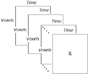
Shenton, Dickey, Frumin & McCarley, 2001), can be arranged in a three-dimensional array in which voxels represent the first dimension, time points the second and subjects the third one. As can be seen in Figure 1, multi-subject fMRI data can also be considered as multiple two-dimensional matrices (i.e., voxels by time points) where each matrix represents the fMRI data of a single individual.

Figure 1. Graphical representation of multi-subject (resting-state) fMRI data consisting of 𝐼 data blocks with each data block 𝑿𝑖 containing the BOLD response for subject 𝑖 measured for different voxels over time.

(7)

2

disorder, like, for example Alzheimer’s disease, may substantially advance the scientific

knowledge on the neural basis of such a disorder. An often used technique to disclose the most apparent connectivity patterns in resting-state fMRI data of a single subject is

Independent Component Analysis (ICA; see Hyvärinen & Oja, 2000; Stone, 2004; Greicius, Srivastava, Reiss & Menon, 2004; Van de Ven, Formisano, Prvulovic, Roeder & Linden, 2004; Kiviniemi, Knatola, Jauhiainen, Hyvärinen & Tervonen, 2003). ICA is a relatively new decomposition technique that separates a multivariate signal (e.g., fMRI data) into statistically independent components. Moreover, ICA also discloses how the observed signal is obtained as a linear mixing of the underlying independent components (i.e., a linear mixing matrix). In the context of fMRI data, the independent components refer to spatial maps that can be interpreted as sets of voxels that are functionally connected (i.e., connectivity patterns), whereas the mixing matrix contains information regarding the underlying time course for each independent component. An advantage of using ICA (compared to using the linear model) for analysing fMRI data is that the underlying time courses should not be known in advance as they are determined during the analysis; this is especially interesting when working with resting-state fMRI data for which no expectations regarding the true time course of the BOLD signal can be postulated.

When analysing fMRI data of multiple subjects, one analysis strategy consists of performing ICA on each data set separately. A major drawback of such an approach is that the relationships (i.e., systematic differences and similarities) between different subjects are totally neglected. In particular, applying a separate ICA for each subject results in time courses and spatial maps that are specific for each subject, which makes it a difficult task to

(8)

3 Although tensor PICA is clearly able to identify the similarities (i.e., group spatial maps) between the subjects under study, the method may obfuscate relevant differences across subjects. In particular, by assuming spatial maps to be the same for all subjects and time courses to be proportional to each other, crucial (qualitative) differences among the subjects may be overlooked. This may happen, for instance, when the population under study consists of groups of subjects that exhibit qualitative differences in brain functioning. In this regard, one may, for example, hypothesize that different stages of a disorder (e.g., Alzheimer) are characterized by substantial changes in functional connectivity patterns (i.e., spatial maps; see Gili et al., 2011). When this is true, it can be assumed that patients that are in a similar stage of a specific disorder have similar functional connectivity patterns, whereas patients that are in a different stage of this disorder may be characterized by connectivity patterns that are qualitatively different. In this case, a method that is able to identify qualitative differences in functional connectivity between groups of patients would provide a clear advantage over tensor PICA. In particular, such a method may account for the heterogeneity in functional connectivity patterns across (groups of) patients with a certain neurological disorder and, as such, may yield valuable insights into the development and prognosis of the pathology under study.

A promising way to uncover qualitative differences in functional connectivity between

(groups of) patients consists of clustering (in an unsupervised way) the patients based on their underlying brain connectivity patterns. In particular, patients with similar connectivity

patterns should be clustered together, whereas patients exhibiting connectivity patterns that are qualitatively different should be allocated to different clusters. Up to now, however, no such method exists that is able to disclose groups of patients that differ in functional

connectivity patterns. The goal of this master thesis therefore is to develop a novel analysis method for multi-subject fMRI data that combines exploratory clustering techniques (i.e., unsupervised learning) with ICA in order to identify differences in connectivity patterns among (groups of) patients. In particular, the proposed method, which will be called Clusterwise Independent Component Analysis (C-ICA), will cluster the subjects into

(9)

4 functional connectivity instead of or above changes in psychological and behavioural aspects of patients’ functioning); these insights may complement or even contradict the existing

consensus on the disease phases, which are often based on psychological and behavioural aspects of the functioning of the patients only.

The remainder of this thesis, which will be written in the format of an article, is organized as follows: in the next section, the basic principles of ICA estimation for single-subject fMRI data will be discussed and additionally the mathematical formulation of the new C-ICA model will be introduced. Next, in the Data Analysis section, an appropriate algorithm to estimate the parameters of the C-ICA model will be presented, along with a short

description of easy to use software for C-ICA and a procedure to select the optimal C-ICA model (i.e., number of clusters and components needed). In the fourth section, the

(10)

5

Section 2. Clusterwise Independent Component Analysis

In this section, an extensive formulation of the basic ICA model for single-subject fMRI data will be given. Here, several statistical principles and methods for ICA estimation will be explained. Finally, a short motivation for the novel C-ICA model will be presented, alongside the mathematical formulation of the C-ICA model.

2.1 The Independent Component Analysis framework for a single subjects’ fMRI data

2.1.1 Linear representations of multivariate data

A commonly used analysis technique that is able to extract underlying patterns of functional connectivity from the resting-state fMRI data of a single subject is Independent Component Analysis (ICA; Hyvärinen & Oja, 2000; Stone, 2004). In ICA, a multivariate – observed – signal (e.g., the BOLD response for a set of voxels) is decomposed into a set of statistically independent – unobserved – source signals (e.g., correlated voxels which represent

functionally connected brain regions) with their associated time courses. As such, ICA is able to separate systematic signal information (e.g., connectivity patterns, which usually appears in independent components) from noise and other – systematic but not relevant for the study – sources of variability (e.g. subtle head movements, cardiac pulsations) that usually

compromise the BOLD signal.

Technically, ICA is a multivariate analysis technique that aims at finding a linear representation of non-Gaussian data in such a way that the statistical dependency between the

underlying non-Gaussian components is minimized. In the basic ICA model (Jutten &

Herault, 1991; Comon, 1992; Bell & Sejnowski, 1995; Hyvärinen & Oja, 2000; Stone, 2004), an (underlying) 𝑛-dimensional random vector of non-Gaussian independent source signals1 s= (𝑠₁, … , 𝑠_𝑛)T_{is recovered from an 𝑛-dimensional random vector of observed signal}

mixtures x= (𝑥1, … , 𝑥𝑛)T. The observed mixture signals in 𝒙 are obtained by a linear mixing

(11)

6

by means of an 𝑛 × 𝑛 mixing matrix 𝑨 (with elements 𝑎𝑖𝑗) of the (independent) source signals

in 𝒔. Thus, the general ICA decomposition can be written as:

𝒙 = 𝑨𝒔 (2.1)

It should be noticed that in the formulation of ICA (2.1) presented above, the mixing matrix 𝑨 is considered to be square (i.e., 𝑛 source components are derived from 𝑛 mixture signals). In

some applications, however, the goal may be to derive only 𝑞 source signals from 𝑛 observed mixture signals (with 𝑞 < 𝑛), resulting in a non-square mixing matrix 𝑨 (of size 𝑛 × 𝑞). In the non-square case, 𝒙 cannot be perfectly decomposed into the product 𝑨𝒔 and 𝒔cannot be

computed through inverting the mixing matrix (see further). However, a decomposition into 𝑨𝒔 (with 𝒔 containing 𝑞 <𝑛 independent signals) can be sought that approximates 𝒙 as close

as possible (for example, in least-squares sense).

The unknown source signals 𝒔can be computed by multiplying the inverse of the mixing matrix 𝑨(i.e. unmixing matrix 𝑾with elements 𝒘𝑖𝑗) with the observed mixed signals

𝒙:

𝒔 = 𝑾𝒙 (2.2)

Therefore, in order to find the underlying components 𝒔, the unmixing matrix 𝑾 has to be determined. To this end,several statistical principles could be used(for an overview of

different principles, see Hyvärinen and Oja, 2000). For example, one could determine 𝑾 such that the components are uncorrelated with each other. This procedure is known as principal component analysis (PCA). ICA, however, uses a more stringent statistical principle than the principle of uncorrelatedness that is adopted in PCA. In ICA, 𝑾 is determined such that the underlying components are statistically independent from each other.Note that when the components are normally (i.e., Gaussian) distributed, uncorrelatedness implies independence (and vice versa); in the non-Gaussian case, however, independence implies uncorrelatedness but the reverse in general does not hold. Here, two important assumptions are necessary to make ICA estimation and the disclosure of the underlying components possible: (1) the underlying source signals are mutually statistically independent and (2) the underlying source signals are random variables from a distribution that does not resemble the Gaussian

distribution.2

2_{For fMRI data, components pertaining to important systematic information in the signal are often non-Gaussian}

(12)

7

2.1.2 Principles of ICA estimation: independence and non-Gaussianity

Independence. The first principle that is used to estimate ICA is statistical independence. In particular, the source signals 𝒔 are estimated such that they are as independent as possible. Intuitively, the source signals 𝒔 are said to be independent when information on the value of 𝑠_𝑖 yields no information on the value of 𝑠_𝑗 for 𝑖 ≠ 𝑗 (Hyvärinen & Oja, 2000). More formally,

statistical independence can be defined in terms of the joint and marginal probability density functions (pdf) of the 𝑠_𝑖‘s. Statistical independence implies that the joint pdf of 𝒔 equals the product of its marginal pdfs (i.e., the pdfs of the 𝑠𝑖‘s). In particular, consider two random (centered) variables 𝑠₁and𝑠₂, let their joint pdf be denoted by 𝑝𝑠1𝑠2(𝑠1, 𝑠2)and their marginal

pdfs by 𝑝_𝑠1(𝑠₁)and𝑝_𝑠2(𝑠₂), then statistical independence is defined as: 𝑝_𝑠1𝑠2(𝑠₁, 𝑠₂) = 𝑝𝑠1(𝑠1)𝑝𝑠2(𝑠2).3

In practice, however, the exact pdf of a random variable is often unknown and lots of data are required to estimate such a pdf in an accurate way. As a way out, the expectation (of some function) of a given random variable, which can be easily estimated directly from the data, is derived and is used to check for statistical independence (Hyvärinen, Karhunen & Oja, 2001). For a given function 𝑔, the expected value of a function of the (continuous, centered) random variable 𝑠₁ is defined as:

𝐸{𝑔(𝑠1)} = ∫ 𝑔(𝑠1)𝑝𝑠1(𝑠1)𝑑𝑠1

∞

−∞ (2.3)

In the case of two random variables 𝑠1 and 𝑠2, given (arbitrary) functions 𝑔1and 𝑔2, the

expected value of the joint density is given by:

𝐸{𝑔₁(𝑠₁)𝑔2(𝑠2)} = ∫ ∫ 𝑔_−∞∞ _−∞∞ 1(𝑠1)𝑔2(𝑠2)𝑝𝑠1𝑠2(𝑠1, 𝑠2)𝑑𝑠1𝑠2 (2.5)

Here the random variables 𝑠₁ and 𝑠₂ are said to be independent if and only if the expectation (i.e., first moment) of their joint pdf can be factorized into the (product of the) expectations of their marginal pdfs as follow:

𝐸{𝑔1(𝑠1)𝑔2(𝑠2)} = ∫ ∫ 𝑔_−∞∞ _−∞∞ 1(𝑠1)𝑔2(𝑠2)𝑝𝑠1𝑠2(𝑠1, 𝑠2)𝑑𝑠1𝑠2 (2.6)

= ∫ 𝑔1(𝑠1)𝑝𝑠1(𝑠1)𝑑𝑠1 ∞

−∞ ∫ 𝑔2(𝑠2)𝑝𝑠2(𝑠2)𝑑𝑠2 ∞

−∞

= 𝐸{𝑔1(𝑠1)}𝐸{𝑔2(𝑠2)}

Additionally, if 𝑠1and 𝑠2 are independent then their covariance (i.e., joint variability) equals

zero since 𝐶𝑂𝑉 = 𝐸{𝑔1(𝑠1)𝑔2(𝑠2)} − 𝐸{𝑔1(𝑠1)}𝐸{𝑔2(𝑠2)}. Note that in case of statistical

independence both properties hold for any possible functions 𝑔₁and 𝑔₂.

3_{In the case of}_𝑛_{random variables, the joint pdf is a product of}_𝑛_{terms, that is,}_𝑝

𝒔(𝑠1, 𝑠2, … , 𝑠𝑛) =

(13)

8

As mentioned earlier, statistical independence (the property used in ICA) is more stringent than uncorrelatedness. Indeed, uncorrelatedness is obtained when equation 2.6 holds for all linear functions 𝑔1 and 𝑔2, whereas statistical independence requires that 2.6 holds for

all possible functions/transformations 𝑔₁ and 𝑔₂ (Hyvärinen, Karhunen & Oja, 2001), with the class of linear functions being a subclass of the latter (much larger) class of functions.

Non-Gaussianity. A second principle that is used for ICA estimation is that of

non-Gaussianity. For ICA estimation, it is not only necessary that the source signals 𝒔 are assumed to be independent (see above) but the source signals 𝒔 should also be non-Gaussian (i.e., follow a distribution that does not resemble the Normal distribution, like, for example, a Laplace or a uniform distribution). When components are Gaussian, by the Central Limit Theorem, any linear mixture of them is also Gaussian. As such, the underlying components cannot be identified in a unique way from the observed mixtures without extra knowledge regarding these underlying sources. Note that ensuring the components to be independent does not help as in the Gaussian case uncorrelatedness implies independence (and, as a consequence, ensuring independence does not imply a more stringent assumption). In fact, a multivariate distribution of independent (i.e., uncorrelated) Gaussian variables results in a density that is rotationally symmetric (Hyvärinen, Karhunen & Oja, 2001). A density that is rotationally symmetric contains no information about the directions of the columns of the mixing matrix 𝑨, or likewise the unmixing matrix 𝑾 (see equation 2.1 and 2.2 respectively), resulting in the elements in matrix 𝑾 not being identifiable when independent components are Gaussian. Indeed, applying ICA estimation while the underlying components are in fact Gaussian will only result in a whitening of the data (i.e. yields uncorrelated components with unit variances) but does not yield a disclosure of the underlying independent components.

When the underlying independent components are in fact non-Gaussian, then ICA estimation is possible. Given, as following from the Central Limit Theorem, that the

probability density function of a linear mixture of variables is approximately more Gaussian than the pdf of its constituent (source) variables, non-Gaussian independent components 𝒔 can be estimated from their (more Gaussian linear) mixtures 𝒙 by means of maximizing a measure of non-Gaussianity of thesource signals 𝒔. In this procedure, a linear combination 𝑠_𝑗 =

∑ 𝑤_𝑖 _𝑖𝑗𝑥_𝑖 is sought such that the 𝑠_𝑗’s are as Gaussian as possible. To this end, the

non-Gaussianity of 𝑠𝑗 is quantified and this measure is optimized (see further in Section 2.1.3). It

(14)

9 independent components 𝒔 (Hyvärinen, Karhunen & Oja, 2001).

2.1.3 Maximizing non-Gaussianity to ensure independence and the fastICA algorithm

In order to retrieve the independent non-Gaussian signals 𝒔 that underlie a set of observed mixture signals 𝒙, both a measure of the non-Gaussianity of the source signals 𝒔 and an optimization algorithm for maximizing this measure for non-Gaussianity are necessary. A classical measure of non-Gaussianity is kurtosis, which can be defined as the fourth moment 𝐸[𝑠4_]_with_𝑠_{having unit variance and being zero-mean centered. Kurtosis is equal to zero for}

Gaussian random variables, negative for sub-Gaussian (platykurtic) and positive for super-Gaussian (leptokurtic) random variables. A drawback of using kurtosis as an objective function for ICA estimation is that it is very sensitive to outliers (Huber, 1985). Therefore, several other methods have been proposed to estimate ICA, with these methods being based on various approaches. For example, the infomax principle (Bell & Sejnowski, 1995) that is based on a maximum likelihood formulation of ICA can be used to estimate the ICA model. Another approach for estimating ICA consists of computing higher-order cumulant tensors (i.e., a generalization of calculating a covariance matrix) and finding the underlying

components through a kind of eigenvalue decomposition. A popular algorithm in this regard is the JADE algorithm (Cardoso & Souloumiac, 1993). A third commonly used approach for identifying independent components, which will be used throughout this thesis, is maximizing negentropy. This quantity is related to differential entropy, a concept derived from information theory. A variable having a larger amount of “randomness” is said to have a larger entropy.

From all (distributions of) random variables that have the same variance, Gaussian variables have the largest entropy. Negentropy, which is a normalized version of entropy, is always positive and equals zero if and only if a random variable is Gaussian. Further, negentropy is invariant to linear transformations (Comon, 1994; Hyvärinen, 1999; Hyvärinen & Oja, 2000).

As noted in Hyvärinen and Oja (2000), estimation of negentropy is a very difficult and noise-prone task as an (parametric or non-parametric) estimate of the full pdf is necessary. Therefore, Hyvärinen (1998, 2000) proposed to maximize an approximation of negentropy which is less computational intensive:

𝐽(𝑠) ≈ 𝑘₁(𝐸{𝐺₁(𝑠)})2_{+ 𝑘}

2(𝐸{𝐺2(𝑠)}2− 𝐸{𝐺2(𝑣)})2 (2.7) here, 𝑣 is a standardized Gaussian variable, 𝑠 is the independent component that is sought for, 𝑘₁ and 𝑘₂ are positive integers and 𝐺₁ and 𝐺₂ are non-quadratic contrast function that are

(15)

10 𝐺₁(𝑠) =_𝑎1

1log cosh 𝑎1𝑠, where 1 ≤ 𝑎1≤ 2 (2.8)

and,

𝐺₂(𝑠) = −exp(−𝑠2_{⁄ )}₂ _(2.9)

In cases where only one non-quadratic function 𝐺(𝑠) is used, the approximation from Equation 2.7 becomes:

𝐽(𝑠) ∝ [𝐸{𝐺(𝑠)} − 𝐸{𝐺(𝑣)}]2 _(2.10)

where 𝐺(𝑠) can be substituted by either Equation 2.8 or by Equation 2.9.

Equation 2.8 is a general purpose contrast function, meaning that it is suitable for both sub-Gaussian and super-Gaussian components. Equation 2.9, at the contrary, is more suitable when components are known to be highly super-Gaussian and/or when robustness is

important (Hyvärinen, 1999). Note that when it can be expected that the data contain no outliers, kurtosis can be used as a third contrast function:

𝐺₃(𝑠) =1₄𝑠4 _(2.11)

As the components are independent of each other, the optimization of the

approximation of negentropy as presented in (2.7) and (2.10) can be performed by estimating all independent components simultaneously or by using a deflation procedure in which each of the independent components in 𝒔 = 𝑾𝒙is computed separately/sequentially (i.e., the optimization function has different maxima, with each maximum pertaining to a separate independent component; see Hyvärinen, Karhunen & Oja, 2001; Stone, 2004). In particular, for each component separately, a weight vector w is sought, by means of rotating 𝒘, such that the orientation of w gives a maximum value of the negentropy approximation for the extracted component. To find the optimal rotation of 𝒘, different approaches have been proposed. A first approach consists of using a brute force search (Stone, 2004), but this will become easily computationally intensive when more than two components need to be extracted. A solution here is to use a well-known optimization algorithm, like, for example, a gradient descent type of algorithm (Amari, Cichocki & Yang, 1996). Alternatively, Hyvärinen (1999) introduced

(16)

11 may heavily depend on the choice of this step parameter. Note that a deflational procedure for ICA estimation closely resembles another multivariate method, called project pursuit, where projections of multivariate data are found that display interesting (i.e. non-Gaussian)

information/distributions (Friedman, 1987; Huber, 1985) in the data. Extracting components one by one can be used for exploratory data analysis. Moreover, it also decreases

computational load (Hyvärinen & Oja, 2000), which can be very advantageous when, for example, analyzing computationally challenging neuroimaging data sets.

In sum, the problem of finding a suitable linear representation of multivariate non-Gaussian data can be solved by using the statistical principles of statistical independence and non-Gaussianity. Additionally, after determining a measure that quantifies non-Gaussianity, an algorithm can be constructed that optimizes this measure for each component separately. In this thesis, non-Gaussianity will be measured by (an approximation of) negentropy (2.7) and

fastICA will be used to optimize negentropy in a computationally efficient way.

2.2 Clusterwise Independent Component Analysis

In this section, the novel C-ICA model will be presented to uncover qualitative differences in functional connectivity patterns between groups of patients. In this model, the patients are clustered into homogenous groups based on the similarities and differences in the functional connectivity patterns underlying the data of each patient. To determine the connectivity patterns that are common for each patient group, ICA is performed on the concatenated data per group. A similar clustering strategy for identifying heterogeneity in the underlying

association structure of multivariate data has already been successfully adopted in the context of simultaneous component analysis (De Roover, et al., 2012) and for Parafac (Wilderjans & Ceulemans, 2013).

2.2.1 Mathematical model formulation of C-ICA

In the C-ICA model it is assumed that 𝐼 data blocks 𝑿_𝑖 (𝑖 = 1, … , 𝐼 ) fall apart into 𝑅 mutually exclusive clusters, with each data block 𝑿𝑖 containing the fMRI data (𝐽 voxels by 𝐾 time

(17)

12

block (i.e., patient) but the spatial maps are set equal for all data blocks that belong to the same cluster. Thus, C-ICA is defined as:

𝑿_𝑖 = ∑ 𝒑_𝑖𝑟𝒔𝑟_𝑨 𝑖 𝑅

𝑟=1 + 𝑬𝑖 (2.12)

where the elements 𝒑_𝑖𝑟 denote the entries from the binary partition matrix 𝑷 (𝐼 × 𝑅) which equal 1 when data block/person 𝑖 is assigned to cluster 𝑟 and 0 otherwise. Similar as in equation (2.1), 𝑨_𝑖 (𝑄 × 𝐾) denotes the mixing matrix for subject 𝑖 and 𝒔𝑟 (𝐽 × 𝑄)the (independent) source signals for cluster 𝑟 (𝑟 = 1, … , 𝑅). Note that the signals in 𝒔𝑟_are

assumed to be the same for each data block 𝑖that belongs to cluster 𝑟. Additionally, the model

contains an error term 𝑬_𝑖 for each data block 𝑖.

2.2.2 Ambiguities of the (C-)ICA model

The C-ICA model suffers from four sources of non-uniqueness/ambiguity (see Hyvärinen & Oja, 2000; Hyvärinen, Karhunen & Oja, 2001), with the first three also holding for the ICA model and the fourth one being specific for C-ICA. First, scaling ambiguity, which implies that scaling components in 𝒔𝑟 can be compensated in 𝑨_𝑖 by counterscaling, resulting in the product 𝒔𝑟𝑨𝑖 being unchanged. This is because in ICA both the mixing matrix and the independent components have to be estimated and their product shows up in the ICA (and C-ICA) model formulation (2.1). Here, any scalar multiplier applied to one of the sources 𝒔𝑞 can

be cancelled in 𝒔𝑟𝑨_𝑖 by dividing the corresponding row 𝒂_𝑞 of 𝑨 by that scalar. As noted by

Hyvärinen, Karhunen & Oja (2001), this non-uniqueness can be accounted for during ICA estimation by assuming that the independent components 𝒔 all have unit variance (i.e., 𝐸{𝑠_𝑞2_{} = 1}_{). A second ambiguity is reflectional ambiguity, which pertains to the possibility to}

change the sign of an estimated independent component. Indeed, multiplying one of the estimated components (in 𝒔𝑟) by -1 does not affect the ICA model (2.1) as long as this is compensated for in the associated 𝑨_𝑖’s (i.e., multiplying the associated time course with -1). Note that reflectional ambiguity is a special case of scaling ambiguity (i.e., scaling with a factor of -1). Fixing the variance of the independent components, however, does not solve for reflectional ambiguity. Third, since both the components 𝒔 and mixing matrix 𝑨 are unknown, the order of the components in the ICA model can be freely interchanged. To see why this is

(18)

(19)

14

Section 3. Data Analysis

3.1 Aim of C-ICA

Given a pre-specified number of clusters 𝑅 (and, in the non-square mixing matrix case – see earlier – an a priori determined number of components 𝑄), the aim of C-ICA is to estimate a

partitioning matrix 𝑷, mixing matrices 𝑨_𝑖(𝑖 = 1, … , 𝐼) and source signals 𝐬𝑟_{(𝑟 = 1, … , 𝑅)}

such that the C-ICA loss function is minimized:

𝐿 = ∑ ‖𝑿_𝑖 − ∑𝑅 𝒑_𝑖𝑟

𝑟=1 𝒔𝑟𝑨𝑖‖2 𝐼

𝑖=1 (3.1)

Based on the value of the loss function 𝐿, for a particular C-ICA model (with estimates for 𝑷, 𝑨𝑖 and 𝒔𝑟), a percentage of variance accounted for (VAF) can be computed as follows:

𝑉𝐴𝐹 =‖𝑿‖ 2

−𝐿

‖𝑿‖2 × 100 (3.2)

where ‖𝑿‖2 indicates the sum of all squared elements (across all data blocks).

Before analysing a data set with C-ICA, it is advised to pre-process the data by row-wise centring each data block 𝑿_𝑖. As a consequence, for each subject 𝑖, the data for each voxel 𝑗 have a mean of zero (across the 𝐾 time points). Note that this is in accordance with ICA

being defined for centred signals 𝒙 (see Section 2.1.1).

3.2 The algorithm for C-ICA and software

In order to achieve an optimal clustering with the C-ICA model (and to determine the

associated subject specific mixing matrices and group specific source signals), an alternating

(20)

15 1. Randomly initialize partition matrix 𝑷. Here each data block 𝑖 is allocated to one of

the clusters 𝑟, with all blocks having the same probability of being assigned to each cluster. Note that this procedure is repeated until none of the clusters is empty. After the initialization of 𝑷, the cluster specific ICA parameters are estimated as explained in step 3 and the loss function (3.1) is evaluated.

2. Update partition matrix 𝑷 data block by data block. Here the optimal cluster membership for data block 𝑖is determined by evaluating for each cluster 𝑟 the fit of

the data block 𝑖 under consideration by means of the partition criterion 𝐿_𝑖𝑟 =

‖𝑿𝑖 − 𝑿̂ ‖𝑖 2; each person 𝑖 is assigned to the cluster 𝑟 for which 𝐿𝑖𝑟 is minimal. More

specifically, here for each data block 𝑖 in cluster 𝑟an estimated𝑿̂𝑖 is computed via the

formula 𝑿̂ = 𝒔𝑖 𝑟𝑨𝑖, where 𝒔𝑟 is given by the previous fastICA estimation under step 3

and 𝑨_𝒊 is computed via 𝑨_𝑖 = 𝑿_𝑖𝑇_𝒔𝑟_(𝒔𝑟𝑇_𝒔𝑟₎−1_{and (… )}−1_{denotes matrix inversion and}

𝒔𝑇_{the transpose of a matrix/vector. Note that aft}_{er reassigning all data blocks to their}

optimal cluster, it could occur that some clusters are empty. In order to avoid empty clusters, a procedure is applied that puts the data block with the worst fit (after reassigning all data blocks and updating the cluster specific ICA parameters) into the empty cluster.

3. Estimate the ICA parameters for each cluster (and evaluate the loss function). First, all data blocks that belong to cluster 𝑟are horizontally concatenated together into 𝑿𝑟. Next, fastICA is performed on each of the concatenated data blocks 𝑿𝑟in order to estimate the C-ICA parameters𝑨_𝑖 and 𝒔𝑟. Here, fastICA uses the contrast function from equation (2.8) with an alpha value of 1 as this contrast function is suitable for both sub-Gaussian and super-Gaussian components (Hyvärinen and Oja, 2000).After computing the cluster specific ICA parameters, the loss function is evaluated.

4. Convergence criterion. Steps 2 and 3 are repeated until the decrease in the loss

function value (3.1) between two evaluations is smaller than the convergence criterion of .000001.

(21)

16 aim of this procedure is to minimize the possibility that a local optimum of the C-ICA loss function is retained.

Implementation of the C-ICA algorithm in R software. The C-ICA algorithm and the procedure for model selection (see Section 3.3) are implemented in R-code (R Core Team, 2014). To perform the ICA on the concatenated data for each cluster, the ICA-function in the R package ‘fastICA’ is used (Marchini, Heaton & Ripley, 2013). To enforce the statistical

independence of the source signals, this ICA-function optimizes negentropy by means of the fast and robust fixed-point fastICA algorithm (Hyvärinen, 1999).

3.3 Model selection

When performing C-ICA, the number of clusters 𝑅 should be specified a priori. In general, however, no a priori information regarding the optimal number of clusters is present. A way

to determine this number consists of running C-ICA with increasing numbers of clusters (e.g., from one up to six) and using a model selection heuristic to identify the optimal number of clusters. To this end, the CHull procedure (Wilderjans, Ceulemans, & Meers, 2013), which aims at finding a model that optimally balances model fit and model complexity, is proposed. In particular, CHull determines the hull solutions at the boundary of the convex hull of a model mis(fit) by model complexity plot in which all fitted solutions are presented. A final solution is retained by making a scree plot (Cattell, 1966)of the hull solutions and selecting in an automated way the solution lying at the elbow of this plot (for more information, see Wilderjans et al., 2013). To quantify model (mis)fit, the (optimal) value of loss function 𝐿 is adopted, while different options exist to compute model complexity (e.g., the number of clusters, the number of estimated parameters). Note that when a decomposition into a smaller number of components is aimed at (i.e., non-square mixing matrix 𝑨, see Section 2.1.1), also

(22)

17 optimal 𝑅, the optimal number of components 𝑄 (for similar procedures, see De Roover, Ceulemans & Timmerman, 2012; Wilderjans and Ceulemans, 2013). In both steps, a procedure based on scree ratios may be used to determine the optimal number of

clusters/components in an automated way. Here, for the first step, the scree ratio for a certain number of clusters 𝑟 (keeping the number of components fixed at 𝑞) is computed as follow:

𝑠𝑟𝑟|𝑞 = 𝐿_𝐿𝑟−1,𝑞−𝐿𝑟,𝑞

𝑟,𝑞−𝐿𝑟+1,𝑞 , (3.3)

where 𝐿 is the loss function value from equation (3.1) for a C-ICA model with 𝑟 clusters and 𝑞 components4. After computing equation (3.3) for each possible 𝑟 (𝑟 = 2, … , 𝑅_𝑚𝑎𝑥− 1) and

each 𝑞(𝑞 = 1, … , 𝑄_𝑚𝑎𝑥), the optimal number of clusters 𝑅 is determined by averaging 𝑠𝑟_𝑟|𝑞

over all considered number of components 𝑞 and selecting the number of clusters 𝑟 that has the largest averaged 𝑠𝑟_𝑟|𝑞-ratio. Next, in the second step, conditional upon the optimal number

of clusters 𝑅 derived in step 1, the optimal number of components 𝑄 is determined by selecting the number of components 𝑞(𝑞 = 2, … , 𝑄_𝑚𝑎𝑥 − 1) that maximizes the following 𝑠𝑟_𝑞|𝑅-ratio:

𝑠𝑟𝑞|𝑅 = _𝐿𝐿𝑞−1,𝑅−𝐿𝑞,𝑅

𝑞,𝑅−𝐿𝑞+1,𝑅 (3.4)

As in all model selection procedures, the final decision about model retention should also be based on the interpretability of the C-ICA solution.

4_{Note that in the first step it is not possible to compute a scree ratio for the smallest (i.e.,}_{𝑟 = 1}_{) and largest (i.e.,}

(23)

18

Section 4. Simulation studies

In this section, three simulation studies are presented in which the performance of the C-ICA algorithm in terms of recovering the true partition and cluster specific ICA parameters is evaluated. In the first simulation study, the algorithm is tested when a correct number of clusters and independent components are specified for C-ICA. In the second simulation study, the performance of the C-ICA algorithm is examined under less favourable analysis

conditions. In particular, here an incorrect number of clusters is specified. Lastly, a small simulation study is carried out to test the heuristic model selection strategy based on the CHull procedure and the proposed sequential model selection procedure (see Section 3.3). Here, C-ICAsolutions are estimated for several values of 𝑟 and 𝑞 and it is determined whether the proposed model selection procedure identifies the true values for 𝑅 and 𝑄.

4.1 Simulation study 1

4.1.1 Problem

In the first simulation study, the C-ICAalgorithm was evaluated under optimal conditions. In particular, data were generated from a C-ICAmodel with a known true number of clusters 𝑅 and true number of independent components 𝑄 and these generated data sets were subjected

to a C-ICA analysis using the true number of clusters and components. The C-ICA algorithm is evaluated with respect to goodness of recovery, that is, whether (1) the clustering of the data blocks (𝑷) can successfully be recovered, (2) the cluster specific source signals 𝒔𝑟 can be correctly disclosed and (3) the time courses 𝑨_𝑖 can successfully be retrieved.

(24)

19 more noise (Brusco & Cradit, 2005). Finally, regarding the dimensionality of the mixing matrix-factor, no clear expectations are available.

4.1.2 Design and procedure

In order to not have an overly complex design, the number of data blocks was fixed at 40 and only clusters of equal size (i.e., 40 divided by the number of clusters R) were considered. Furthermore, the five aforementioned factors were systematically varied in a full five-factorial randomized design in which all factors were considered as random factors (i.e., the selected values for each factor were considered as sampled at random from a wider population of values):

1. Number of elements in the independent components, at two levels: 500 and 2000 2. Number of independent components 𝑄, at three levels: 2, 5 and 20

3. Number of (equally sized) clusters 𝑅,at two levels: 2 and 4

4. Dimension of mixing matrices 𝑨𝑖, at 2 levels: square or non-square 5. The amount of noise E in the data, at three levels: 5 %, 20 % and 40 %.

With regard to the fourth factor, in the case of a square mixing matrix, the dimensionality of 𝑨_𝑖 depends on the number of independent components 𝑄 (i.e., either 2x2, 5x5 or 20x20). In

the non-square conditions, however, the number of observed mixtures was held constant at 64 (i.e., a number larger than the number of independent components), resulting in the mixing matrix being either 2x64, 5x64 or 20x64. Furthermore, as in the general ICA model, the C-ICAmodel assumes that the independent components are non-Gaussian. Therefore the 𝑄 components for a particular cluster specific 𝒔𝑟were independently generated from one of the following four non-Gaussian distributions:

1. Uniform distribution 2. Laplace distribution

3. Bimodal distribution with equal peaks 4. Bimodal distribution with unequal peaks

Note that this implies that all independent components for a particular 𝒔𝑟 were drawn from the same non-Gaussian distribution (e.g., the 𝑄 components of 𝒔1 following a Laplace

distribution). When four clusters were generated, all aforementioned distributions were included (i.e., each of the four 𝒔𝑟 was associated with a different distribution); in the

(25)

20 replacement (i.e., 𝒔1 having one of the four distributions and 𝒔2 having another one).

All independent components were generated using the R function icasamp() from the

ica package (Helwig, 2014). This function ensures that the generated components have a

mean of zero. Moreover, the independent components were mixed with subject specific generated mixing matrices 𝑨𝑖, which were drawn from a uniform distribution with mean zero. Additionally, a noise matrix 𝑬_𝑖 (𝐽 × 𝐾) was added to each data block 𝑿_𝑖 (𝐽 × 𝐾). Here, each noise matrix 𝑬_𝑖 was constructed by independently drawing numbers from 𝑁(0,1). Next, the noise matrices were rescaled to ensure that computed across all data blocks 𝑿𝑖 the data contained the required percentage of noise (i.e., 5%, 20% or 40%).

Lastly, for each cell in the five-factorial design, 10 replication data sets were

generated. Thus, in total, 2 (number of elements) × 3 (number of independent components) × 2 (number of clusters) × 2 (dimension of mixing matrix) × 3 (error) × 10 (replications) = 720 C-ICA data sets were generated. Each data set was analyzed with the C-ICA algorithm with 75 random starts, and the solution with the lowest value on the loss function 𝐿 (see equation 3.1) was retained.

4.1.3 Results

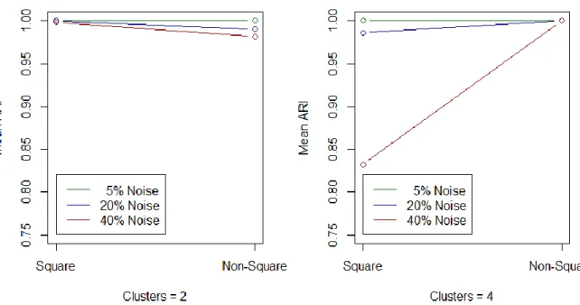
Recovery of the clustering of the data blocks (𝑷). In order to evaluate the goodness of recovery for the clustering of the data blocks, the Adjusted Rand Index (ARI; Hubert & Arabie, 1985) is computed between the true partition of the data blocks and the estimated partition. The ARI equals 1 if two partitions are identical and 0 when the overlap between both partitions is at chance level. The overall mean ARI, across all 720 data sets, equals .9823 (SD = .0714). Moreover, a perfect recovery of the partition was observed for 652 of the 720 data sets (i.e., 90.56%). It can be concluded that the C-ICA algorithm recovers the clustering of the data blocks to a very large extent.

To study how the recovery of the clustering of the data blocks changes as a function of the manipulated factors, Table 1 gives an overview of the mean ARI (and standard deviation of ARI) for each level of the five manipulated factors. From this table it can be seen that when the amount of noise is low (i.e., 5%), a perfect recovery is encountered for each data set. However, recovery slightly deteriorates when the amount of noise in the data increases (i.e.,

(26)

21 square, and (3) the number of elements in the components decreases. For the number of components, best recovery results are obtained for intermediate values of 𝑄.

Table 1. Mean ARI and Tucker’s congruence value (and standard deviation) for all levels of the manipulated factors

Factor Level ARI Tucker’s

Congruence

Number of elements in 500 .9807 (.0716) .8835 (.1019)

independent components 2000 .9840 (.0714) .9033 (.0681)

Number of 2 .9659 (.1046) .9530 (.0515)

independent 5 .9940 (.0308) .9231 (.0380)

components 𝑄 20 .9870 (.0551) .8042 (.0795)

Number of 2 .9950 (.0520) .8935 (.1020)

clusters 𝑅 4 .9696 (.0848) .8933 (.0694)

Dimensionality of Square .9694 (.0849) .8814 (.0879)

the mixing matrix Non-square .9953 (.0518) .9054 (.0849)

Amount of noise 5% 1 (.0000) .8975 (.0805)

in the data 20% .9940 (.0423) .8871 (.0926)

40% .9530 (.1107) .8956 (.0880)

(27)

22 a small number of clusters underlies the data, however, the opposite is observed (see left-hand panel of Figure 2).

Figure 2. Recovery of the clustering of the data blocks (in terms of ARI) as a function of a three-way interaction

between factors Amount of noise, Dimensionality of the mixing matrix and Number of clusters.

Recovery of the independent components (𝒔𝑟). To evaluate the extent to which the true independent components were recovered, for each component separately, the Tucker congruence coefficient (Tucker, 1951) is computed between the simulated independent component and the corresponding estimated independent component. To arrive at a single Tucker congruence value for each 𝒔𝑟-matrix, for each of the 𝑄 components of that 𝒔𝑟 the Tucker value is computed (after accounting for the C-ICA ambiguities – see further) and the mean across these 𝑄 obtained Tucker values is calculated. To obtain a single Tucker value for each generated data set, the (mean) Tucker values of the 𝑅𝒔𝑟’s were averaged. Tucker’s congruence coefficient equals the normalized inner product between two vectors and ranges from -1 to 1, with 1 indicating perfect recovery.5 A value in the range of .85-.94 denotes a fair similarity between the two vectors, whereas a value larger than .95 indicates that the two vectors are very similar (Lorenzo-Seva & ten Berge, 2006).

Determining the extent to which the simulated independent components are recovered by the estimated independent components is not straightforward as the C-ICA model suffers

5

(28)

23 from four ambiguities (see Section 2.2.2): scaling, reflectional and component and cluster permutational freedom.To take these ambiguities into account when computing Tucker’s congruence, the following procedure was followed: (1) the absolute value of the Tucker coefficient is taken to account for reflectional freedom; (2) to account for the permutational freedom of both the components and the clusters, all possible combinations of cluster and component permutations are considered and for each combination of these permutations the associated mean Tucker congruence (averaged across components and 𝒔𝑟’s) is computed. Next, the combination of cluster and component permutation with the largest Tucker

congruence value is retained and the associated averaged Tucker value is reported. Note that as the Tucker coefficient is invariant under a scaling of the components with a positive scalar, this coefficient automatically accounts for the scaling ambiguity of the C-ICA model.

As the overall mean Tucker congruence equals .8934 (SD = .0871), it can be

concluded that the C-ICA algorithm recovers the independent components reasonably well. The mean Tucker congruence value (and standard deviation) for each level of each factor can be found in Table 1. From this table it can be seen that the mean Tucker congruence especially varies as a function of the number of independent components 𝑄, with recovery deteriorating when 𝑄 increases (M = .9530 versus M = .8042 for 2 and 20 components, respectively). Further, recovery of the independent components also decreases when (1) the number of elements in the independent components decreases, (2) the mixing matrix becomes square and (3) the data contain (more) noise.

(29)

24 compared to 4).

Recovery of the time courses (𝑨𝑖). In order to evaluate to what extent the time courses (i.e., mixing matrices 𝑨_𝑖) are recovered, Tucker’s congruence coefficient (Tucker, 1958) is computed between each simulated and estimated mixing matrix. This measure, denoted by Tucker’s mean 𝑨 (TMA), is computed in a similar way as was done for determining the recovery of the independent components, herewith accounting for the C-ICA ambiguities (i.e., scaling and reflectional ambiguity and component permutational freedom but not cluster permutation freedom) in the same way as before (see earlier).

The mean TMA across all data sets is .7419 (SD = .1920). Therefore, it can be

(30)

25 Table 2. Average Tucker’s mean 𝑨 value (and standard deviation) for all levels of the manipulated factors.

Factor Level Tucker’s mean A

(TMA)

Number of elements in 500 .7440 (.1927)

independent components 2000 .7397 (1914)

Number of 2 .9184 (.0871)

independent 5 .7959 (.1180)

components 𝑄 20 .5112 (.0410)

Number of 2 .7442 (.1936)

clusters 𝑅 4 .7395 (.1906)

Dimension of Square .6621 (.1529)

the mixing matrix Non-square .8216 (.1941)

Amount of noise 5% .7454 (.1943)

in the data 20% .7413 (.1918)

40% .7388 (.1905)

4.2 Simulation study 2

4.2.1 Problem and design

In the second simulation study, the performance of the C-ICA algorithm is examined under less favorable conditions, that is, with an incorrect number of clusters. To this end, data were simulated according to the same design and procedure as in the first simulation study, but now only taking 5 replications per cell of the design. Each of the 360 generated C-ICA data sets was analyzed (using 75 random starts) twice: (1) with the true number of clusters 𝑅 and (2) with one cluster too many (i.e., 𝑅+1).

(31)

26 extracted, expectations are that one true cluster will be split into two (or more) subclusters. Additionally, since the C-ICA algorithm ensures that empty clusters do not occur (see section 3.2), it is expected that specifying one cluster too many may result in one estimated cluster containing a single data block. This single data block truly belongs to another cluster, but has the worst fit for that cluster. This behavior of the C-ICA algorithm is especially expected when the data contain no noise (or at least a minimum amount of noise, i.e., 5%) as in that case the optimal partition into 𝑅 + 1 clusters is a clustering where the worst fitting block from the 𝑅 cluster solution is assigned to a separate (singleton) cluster.

4.2.2 Results

The mean ARI across all generated datasets equals .9752 (SD = .0914) when a correct number of clusters 𝑅 is specified. As expected, when one cluster too many is specified (i.e., 𝑅 + 1), the C-ICA algorithm recovers the partitioning of the data blocks to a smaller extent (M = .8992, SD = .0899). From Table 3, in which the mean ARI for each level of each design factor is presented for both 𝑅 and 𝑅+1, it appears that when a correct number of clusters is specified, recovery decreases when (1) the number of independent components 𝑄 decreases, (2) the number of clusters 𝑅 increases, (3) the mixing matrix becomes square, and (4) the data contain more noise. Note that these tendencies have also been observed in the first simulation study. An analysis of variance with ARI as the dependent variable shows a three-way

interaction between the number of clusters, the dimensionality of the mixing matrix and the

amount of noise (𝑝̂ = .23) that has also been found in simulation study 1 (albeit being stronger there). When 𝑅 + 1 clusters are extracted, as can be seen in Table 3, recovery decreases when (1) the independent components have less elements, (2) the number of clusters decreases, and (3) the data are more noisy. Further, an analysis of variance with ARI as the dependent

variable showed a significant five-way interaction effect (𝑝̂ = .19). The overall tendency of this complicated interaction effect can be summarized as follow: the recovery of the clustering – in general – improved when (1) less components were extracted, (2) less noise is present in

the data, and (3) the mixing matrix is non-square. Moreover, when a large number of components was extracted, ARI generally deteriorated when many clusters were underlying the data. This deterioration was more pronounced when the independent components had a smaller number of elements.

(32)

27 when one cluster too many is specified, a dichotomous variable single membership (being 1 when there is one estimated cluster that contains a single member and 0 otherwise) is computed for all 360 C-ICA data sets. As expected, the occurrence of a single data block in one estimated cluster was observed more frequent when noise is minimal (i.e., 73%, 58% and 37%, for 5%, 20% and 40% of noise, respectively).

Further, when only considering the data sets where no single memberships occurred, it was examined how often one true cluster was split into two estimated clusters (as opposed to being split into more than two clusters). Note that this implies that the other 𝑅 − 1 true clusters were recovered perfectly. Results show that when one cluster too many (i.e., 𝑅+1) is estimated, the percentage of data sets where one true cluster is split into two estimated clusters, increases when noise decreases (i.e., 67%, 90% and 100% for 40%, 20% and 5% of noise, respectively).

(33)

28 Table 3. Mean ARI (and standard deviation) for 𝑅 and 𝑅+1 specified clusters (for the same 360 generated C-ICA

data sets) as a function of the manipulated factors.

Factor Level 𝑹 clusters 𝑹 + 𝟏 clusters

Number of elements in 500 .9797 (.0768) .8860 (.0902)

independent components 2000 .9708 (.1039) .9125 (.0879)

Number of 2 .9540 (.1317) .8968 (.0944)

independent 5 .9881 (.0577) .9141 (.0789)

components 𝑄 20 .9836 (.0617) .8868 (.0942)

Number of 2 .9902 (.0758) .8680 (.0904)

clusters 𝑅 4 .9603 (.1027) .9305 (.0779)

Dimension of Square .9603 (.1027) .8973 (.0899)

the mixing matrix Non-square .9902 (.0758) .9012 (.0901)

Amount of noise 5% 1 (.0000) .9219 (.0763)

in the data 20% .9983 (.0107) .9133 (.0758)

40% .9274 (.1470) .8625 (.1037)

4.3 Simulation Study 3

4.3.1 Problem and design

(34)

29 amount of noise in each data block was 5%. Components, mixing matrices and noise were generated as explained before (see Section 4.1.2).

For each of the 4 data sets, a C-ICA was performed with 75 (random) multiple starts and with 𝑞 and 𝑟 both varying from 1 to 5. In each analysis, the solution with the lowest loss function value (3.1) was retained. Thus, in total 4 × 5 × 5 = 100 C-ICA analyses were performed.

To quantify model complexity in the case when the CHull procedure was adopted, the total number of estimated parameters of a C-ICA solution was taken (i.e., total number of estimated elements across all 𝒔𝒓 and 𝑨_𝑖‘s together). Furthermore, the value for loss function 𝐿 (3.1) was used as a measure for model (mis)fit; this value was also used to compute scree ratio values for equations (3.3) and (3.4) in the case when a sequential model selection procedure was adopted.

4.3.2 Results

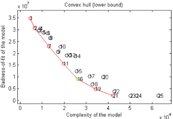
Results show that for the generated C-ICA data sets, the sequential model selection procedure outperforms CHull. In particular, the sequential method identified the correct model (i.e., the model with the true number of clusters 𝑅 and components 𝑄) in three out of four cases, whereas CHull never retained the correct model although the correct model was always located on the boundary of the convex hull. The correct model, however, was always the most complex hull model so that it could not be selected by CHull as CHull cannot select the most simple and the most complex hull model (see Section 3.3). As an illustration of this, Figure 3 shows the CHull plot for the generated data set with 𝑅 = 4 and 𝑄 = 4 (CHull plots for the other data sets are presented in Appendix I, Figures 1-3). In this figure, one can see that CHull erroneously selects a model with 𝑅 = 2 and 𝑄 = 4 (i.e., indicated by a green circle).

(35)

30 Figure 3. CHull plot for the generated data set with four true clusters (𝑅 = 4) and four true components (𝑄 = 4).

C-ICA analyses with 𝑟 and 𝑞 ranging from 1 up to 5 have been performed. The model indicated by a green circle

(𝑅 = 2, 𝑄 = 4) is selected by CHull. Note that the true model is hull model number 21 (𝑅 = 4, 𝑄 = 4).

To illustrate the sequential model selection procedure, the results of this procedure for the generated data set with 𝑅 = 4 and 𝑄 = 4 are presented in Table 4 and Figure 4 (results for the other data sets are presented in Appendix I, Tables 1-2 and Figures 4-5).

Table 4. Sequential procedure applied to the generated data set with four true clusters (𝑅 = 4) and four true

components (𝑄 = 4). Scree ratios 𝑠𝑟𝑟|𝑞 for the number of clusters 𝑟 (𝑟 = 2, … , 𝑅𝑚𝑎𝑥− 1) given the number of

components 𝑞 (𝑞 = 1, … , 𝑄𝑚𝑎𝑥) and the mean scree ratios over components are displayed. The largest scree ratio

in each column is highlighted in bold.

Number of clusters 𝑹

q = 1 q = 2 q = 3 q = 4 q = 5 Mean 𝒔𝒓 over

components

2 3.61 3.40 3.50 3.32 4.05 3.55

3 1.55 1.45 1.46 1.48 1.60 1.51

4 1.71 3.67 7.25 520.54 264.39 159.51

Table 4 shows the computed scree ratios 𝑠𝑟_𝑟|𝑞 from step 1 of the sequential procedure (see

(36)

31 mean 𝑠𝑟𝑟|𝑞= 159.51), the optimal number of clusters equals 4. Only considering C-ICA

solutions with four clusters, the scree ratio values 𝑠𝑟𝑞|𝑅=4 (see equation 3.4) are 1.08, 1.10 and

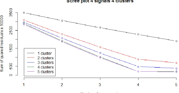
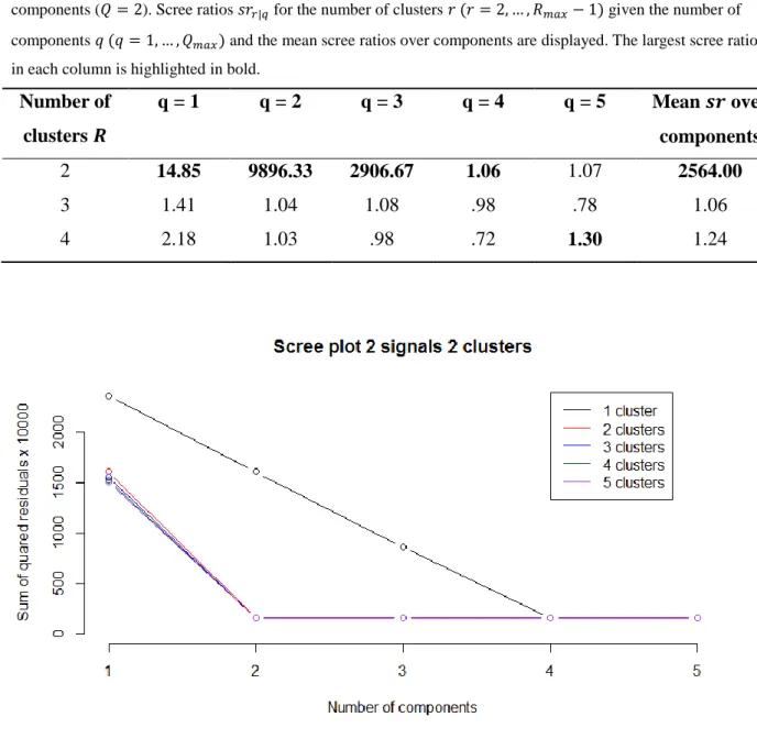
1081.84 for 𝑞 = 2, 𝑞 = 3 and 𝑞 = 4, respectively, resulting in the selection of the solution with four components. Thus, according to the sequential model selection procedure, the model with 𝑅 = 4 clusters and 𝑄 = 4 components should be retained, which is the correct model underlying the data. The same conclusion can be drawn when looking at Figure 4 which shows a scree plot in which the number of components 𝑞 (𝑞 = 1, … ,5) is plotted against the loss function value (3.1) for C-ICA solutions with different numbers of clusters 𝑟 (𝑟 = 1, … ,5). This figure clearly shows that the decrease is the loss function value levels off when

more than 4 components are retained and that the four-cluster solutions fit best.

Figure 4. Scree plot for the generated data set with four true clusters (𝑅 = 4) and four true components (𝑄 = 4) .

For all C-ICA solutions with the number of clusters and components varying between one and five, the number

of components is plotted against the loss function value. Solutions with the same number of clusters are

indicated in the same colour and connected by a line.

(37)

32 this data set. Here the 𝑠𝑟𝑞|𝑅=2 values for the solution with 2, 3, and 4 components are 4.07,

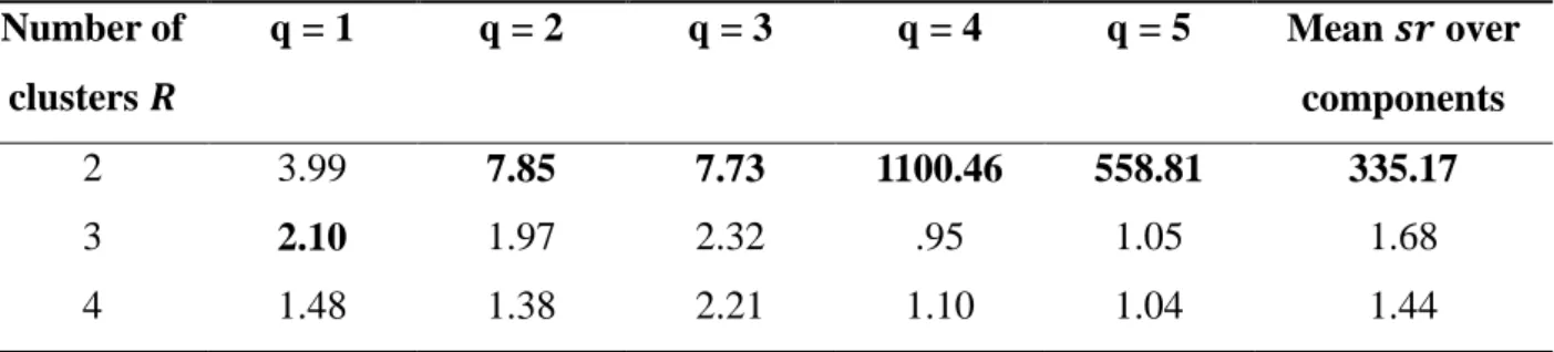
1.15, and 492.54, respectively, resulting in the sequential procedure – incorrectly – indicating that the optimal number of components is 4. As such, the sequential procedure erroneously retains the solution with two clusters (𝑅 = 2) and four components (𝑄 = 4).

Table 5. Sequential procedure applied to the generated data set with four true clusters (𝑅 = 4) and two true

components (𝑄 = 2). Scree ratios 𝑠𝑟_𝑟|𝑞 for the number of clusters 𝑟 (𝑟 = 2, … , 𝑅_𝑚𝑎𝑥− 1) given the number of components 𝑞 (𝑞 = 1, … , 𝑄_𝑚𝑎𝑥) and the mean scree ratios over components are displayed. The largest scree ratio in each column is highlighted in bold.

Number of clusters 𝑹

q = 1 q = 2 q = 3 q = 4 q = 5 Mean 𝒔𝒓 over

components

2 3.77 3.86 6.18 853.61 488.23 271.13

3 4.03 1.23 1.15 1.23 1.46 1.82

4 .31 950.70 281.01 1.33 .76 246.82

However, the scree plot (see Figure 5) for this data set tells a different story. Here, for the number of clusters 𝑟 going from 2 to 5, the decrease in loss functions values cease at 𝑞 = 2 components indicated by the ‘elbow’) and not at 𝑞 = 4 components as suggested in the second step of the sequential procedure. Moreover, the mean 𝑠𝑟 over all components for 𝑟 = 4 (mean 𝑠𝑟 = 246.82; see Table 5) is only a bit smaller than the mean 𝑠𝑟 over

components for 𝑟 = 2 (mean 𝑠𝑟 = 271.13). Computing the scree ratios for 𝑟 = 4 (i.e., 𝑠𝑟𝑞|𝑅=4 equals 2512.78, .85 and 1.05 for the solution with 2, 3, and 4 components,

(38)

33 Figure 5. Scree plot for the generated data set with four true clusters (𝑅 = 4) and two true components (𝑄 = 2) .

For all C-ICA solutions with the number of clusters and components varying between one and five, the number

of components is plotted against the loss function value. Solutions with the same number of clusters are

indicated in the same colour and connected by a line.

(39)

34

Section 5. Discussion

5.1 Discussion of the results

In this master thesis, a new model (C-ICA) was proposed that combines an exploratory

clustering technique with ICA in order to identify differences (and similarities) in connectivity patterns between groups of patients (e.g., patients with Alzheimer’s disease). In this model, patients are clustered into homogeneous groups such that patients in the same group have the same functional connectivity patterns (i.e., captured by the underlying independent

components) and patients belonging to different groups can be characterized by means of connectivity patterns that are qualitatively different. Additionally, to estimate the parameters of the C-ICA model, an alternating least squares type of algorithm was constructed. Further, in order to determine the optimal number of clusters underlying a data set at hand, two model selection procedures were proposed. First, a CHull based procedure that determines the optimal number of components and clusters by balancing model (mis)fit and model

complexity. Second, a two-step (sequential) procedure in which, first, the optimal number of clusters is determined, and, next, conditional on this optimal cluster number, the optimal number of components is selected; an automated scree test like procedure based on computing ratios is used in both steps. Finally, two extensive simulation studies were carried out to evaluate the performance of the C-ICA algorithm in terms of recovering the C-ICA parameters (i.e., the clustering, independent components and mixing matrix) and it was investigated whether performance depends on specific data characteristics. The two proposed model selection procedures were evaluated in a (smaller) third simulation study. In the following, the results of the three simulation studies are summarized and their implications are discussed.

Overview of the results of the three simulation studies. The first simulation study shows that the C-ICA algorithm performs well in recovering the underlying C-ICA parameters when a correct number of clusters 𝑅 and components 𝑄 is selected. As expected, the C-ICA algorithm

performs somewhat worse when the underlying C-ICA model is complex (i.e., consisting of many clusters) and when the data are very noisy. This worse performance, however, only is

(40)

35 al., 2011; Milligan, Soon & Sokol, 1983), C-ICA, however, encounters some difficulties when the complexity of the underlying C-ICA model increases (i.e., more independent

components). Additionally, C-ICA recovers the independent components better when these

components contain a large number of elements and when the mixing matrix is non-square, a result that also has been observed for the recovery of the clustering. Regarding the recovery of the time courses, less good recovery results are obtained. The C-ICA algorithm especially performs weak when the underlying C-ICA model is complex (i.e., having many independent components) and when the underlying mixing matrix is square. Note that square mixing matrices also posed problems for the recovery of the clustering and the independent components.

The main goal of the second simulation study is to evaluate to what end the C-ICA algorithm can successfully recover the true cluster partition when an incorrect number of clusters is specified (i.e., 𝑅 + 1). The results show that when one cluster too many is

specified, the C-ICA algorithm often assigns exactly one data block (i.e., person) to one cluster or splits one true cluster into two (estimated) clusters. The C-ICA algorithm shows this tendency especially when the amount of noise in the data is low.

In the third simulation study, the two proposed model selection procedures are compared to each other for a limited number of data sets. It appears that the sequential

procedure selects the correct model most of the time. When the procedure fails to identify the correct model, the two-step scree ratio test tells a different story than a scree plot analysis, highlighting the need of considering both pieces of information when selecting an optimal model. The CHull procedure always retains a less complex model than the true model. The true model, however, always lies on the convex hull, but is never selected as it is the most complex hull model.

Implications of the simulation results. The simulation studies demonstrated that the C-ICA algorithm uncovers the true partition to a very large extent. The independent components are recovered quite well by C-ICA, but the disclosure of the mixing matrices is not completely satisfactory. The good recovery of the clustering may in part be caused by the fact that true