An Iterative Method for Solving Quadratic
Optimal Control Problem Using Scaling
Boubaker Polynomials
Imad Noah Ahmed
1*, Eman Hassan Ouda
11
University of technology, Baghdad, Iraq
*Corresponding author: Imad Noah Ahmed: [email protected]
Abstract
:
Keywords: Quadratic optimal control problem, State parameterization
technique, Scaling Boubaker function, Iterative method.
Introduction
Optimal control represents a large field in which many researchers gave different methods of various aspects. The crucial aim for solving an optimal control problem (OCP) is to find the control variable which minimizes a given performance index while all the given constraints are satisfied. State parameterization method is one of the mostly used direct methods in solving (OCPs) by the researchers. Kafash B., Delavarkhalafi A. and Karbassi S. M., used state parameterization for solving (NOCPs) and the controlled Duffing Oscillator [1]. Ouda E. H., utilized generalized Laguerre polynomials as a basis function with the aid of state-control parameterization to find an approximate solution for (OCPs) [2].
Scaling functions are a functional dilation equation has the general following form
Citation: Ahmed I.N., Ouda E.H (2020) An Iterative Method for Solving Quadratic Optimal Control Problem Using Scaling Boubaker Polynomials. Open Science Journal 5(2)
Received: 9th June 2020
Accepted: 18th June 2020
Published: 30th June 2020
Copyright: © 2020 This is an open access article under the terms of the Creative Commons Attribution License, which permits unrestricted use, distribution, and reproduction in any medium, provided the original author and source are credited.
Funding: The author(s) received no specific funding for this work
Competing Interests: The author has declared that no competing interests exists.
With a nonzero solution, this kind of equations has been used in many fields (e.g., interpolating subdivision schemes and wavelet theory) [3]. Yousfi S. A., presented a numerical solution of Emden–Fowler equations using Legendre scaling function approximation [4]. Ouda E. and Ahmed I. utilized direct methods (state and control Parameterization) with the scaling Boubaker function for solving OCP[5].
Iterative technique was also largely used for solving OCPs in last decades, Keyanpour M. and Azizsefat M., had an iterative approach with a hybrid of perturbation and parameterized methods for this purpose [6]. Ramezanpour H. et al., presented a new procedure depending on homotopy perturbation method with iterative technique to solve an optimal control problem of a bilinear systems [7]. Elaydi H., Jaddu H. and Wadi M., utilized Legendre scaling function with iterative technique for solving NOCP [8]. Jaddu H. and Majdalawi A., presented an iterative technique in two proceedings, firstly by parameterizing the state variables by finite length Chebyshev series [9], secondly by a finite length Legendre polynomials [10].
Eskandri M. et al., introduced a method for solving a class of nonlinear quadratic optimal control problem (NQOCP) based on variational iteration method [11]. Ramezani M., proposed a new iterative method utilizing 2nd kind Chebyshev wavelet [12]. Shihab S. and Delphi M., used the iterative technique on B-spline Bernestein polynomials [13].
Boubaker polynomials are proved to be a good tool for solving (OCPs), Samaa F. et al., used indirect method based on Boubaker polynomial [14]. Ouda E. H., deduced the operational matrices of derivative and integration and using them with the indirect method [15]. Many other researchers deal with this kind of polynomials in different proceedings. The novelty of our approach is using scaling Boubaker polynomials for solving (QOCP's), this method was proved to be efficient and accurate. A comparison was introduced to show the capability of this method with some other methods.
This paper is arranged as follows, in section2, Boubaker polynomials have been presented. In section3, scaling Boubaker polynomials were introduced. In section 4, the proposed method was presented in steps. In section 5, some numerical examples with comparison for the first example and illustrative figures were added to show the capability of this method, at the end conclusion and the references.
Boubaker polynomials
The Boubaker polynomials were established for the first by Boubaker et al. as a tool for solving heat equation inside physical model, and then it was used for solving different equations in many applications. [16]
Boubaker polynomial is introduced by the following equation [17]
( ) ( 4 ) 2
( ) ( 1) , 0,1, 2,... ...(2)
0 ( )
2 (( 1) 1)
( )! where is , ( ) . !( the de 2 gr
)! 2 4
e
Bn t n n p Cn pp p nt p n
p n p
n
n n
n p p
Cn p n
p n p
m
− − = − − = = − + − − − = = = − −
e of Boubaker polyn
om
The first terms of Boubaker polynomials are
B
0(t) = 1, B
1(t) = t, B
2(t) = t
2+ 2, …
and the recurrence relation
B
m(t) = tB
m-1(t)
−
B
m-2(t
),
wherem > 2
Scaling boubaker polynomials (SBP)
The Scaling Boubaker polynomials (SBP), can be defined as follows [18]
The arguments of scaling (k, n, m, t), k is positive integer, n = 0, 1, 2, 3,..., 2k, m is degree of Boubaker polynomials and t is the time.
Choosing k=1 and m=5. The first five terms Scaling Boubaker SBm(t) were found by using (3) to be:
,
The convergence of this method with state parameterization technique has been treated in [2].
The proposed method
The state parameterization is based on approximating state variables by using Scaling Boubaker polynomials (SBP) with unknown coefficients as follows,
where are unknown coefficients of state
,
SB are the Scaling Boubaker polynomials.
x (t) = a
0SB
0+a
1SB
1+ a
2SB
2+ a
3SB
3+ …+a
nSB
nwith initial condition where the state
coefficients must be found
.
The process steps are
- For the 1st iteration , representing the unknown function x by the first three terms of the scaling Boubaker polynomial with their coefficients
a
i's
on the interval[0,1] asx(t) = a
0SB
0+a
1SB
1+ a
2SB
2…(5)
- Substituting (5) in constraint equation for finding the control variable u with the unknown coefficients
a
i's
.- Using now the performance index to find J, we get a set of algebraic equations with the
a
i's.
which can simply be found by the aid of theinitial conditions.
- Repeating the first iteration with more terms of the scaling Boubaker polynomial for the second and third iterations, evaluating the
J
i's
andcompare their values with respect to
J
exact.- The iterative process continues until a predetermined acceptable error value.
Numerical Examples
Ex.1: Consider the following quadratic optimal control problem [ 19 ] Min
with and .
The exact solution is
, J exact = 0.328258821374830
The results of the 1st Iteration are
x1=(5 /44)t2+(17/44)t + (1/1306897830861018)
u1 = (5/22) t + (17/44)
The results of the 2nd Iteration are
x2 =(7 /86) t3- (4/473) t2+(202 /473)t + (1/317825433919741)
u2= (21/86) t2- (8/473) t + (202/473)
J2= 0.328259337561646
The results of the 3rd Iteration are
x3 =(21 /2242)t4+(145/2314)t3+(115/41138)t2+(483 /1136) t +(1/704329587969285)
u3= (42 /1121) t3+ (435 /2314) t2+ (115 /20569)t + (483/1136)
J3=0.328258830708990
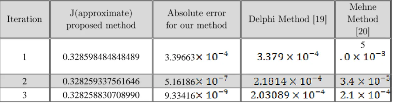
From table1, we noticed that our proposed method has less absolute error with respect to Delphi and Mehne in which power and Bernestein polynomials have been used.
Table 1.The values of cost functional J in Example 1
Iteration proposed method J(approximate) for our method Absolute error Delphi Method [19]
Mehne Method
[20]
1 0.328598484848489 3.39663
5
2 0.328259337561646 5.16186
3 0.328258830708990 9.33416
Figure 3 Example 1 – u variables
Ex.2: Consider the problem [21]
Min , 0
with
The exact solution is
, where
J exact=0.192909298093169
The results of the 1st Iteration are
x1=(100/187) t2-(234 /187)t + 1
u1 = (100/187) t2- (2/11) t – (47/187)
J1= 0.194295900178253
The results of the 2nd Iteration are
x2 =(634 /2775)t3+ (1125 /1283)t2- (757 /554)t + 1
u2 = – (634/2775) t3 + (1965/10264) t2 + (907 /2342) t -203/554
J2= 0.192931605611848
The results of the 3rd Iteration are
x3 =(113 /1297)t4- (772/1917) t3+(1014 /1033) t2-(1128/815)t + 1
u3= (113 /1297) t4-(335/6179) t3- (111 /490) t2+ (1262/2179) t – (313/815)
J3 =0.192909445024077
Table 2 Numerical Results of Example 2
Iteration J(approximate) Absolute error
1
0.194295900178253 1.3866
2
0.192931605611848 2.23075
3
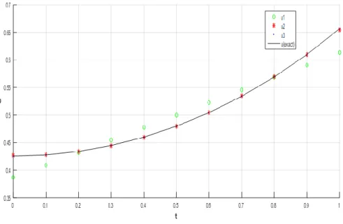
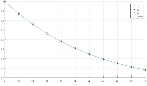
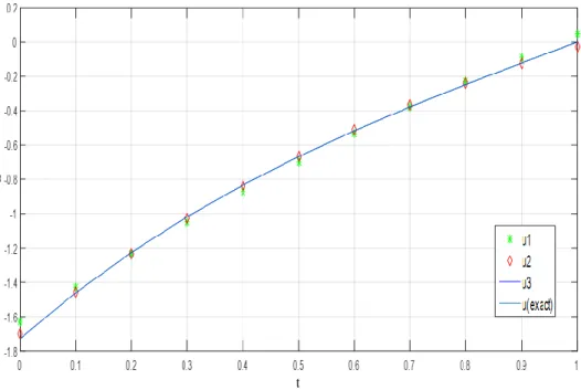
Figure 4 Example 2-x variables
Figure 5 Example 2- u variables
Ex.3: Consider the problem [2]
Min , 0
,
and
The results of the 1st Iteration are
x1 =(54/73)t2- (412/365) t+ 1
u1= (746/365) t - (27/73) t2 – (1189/730)
The results of the 2nd Iteration are
x2 =-(233/1673)t3+ (1067/1126)t2- (625/521)t + 1
u2 = (233/3346) t3- (691/775) t2 + (2001/802) t – (1771/1042)
J2= 0.864218070459266
The results of the 3rd Iteration are
x3 = (295/2182) t4- (841/2053)t3 + (1471/1325) t2- (919/749) t + 1
u3 = - (266/3935) t4+ (1741/2335) t3 – (1586/889) t2+ (2678/945) t – (1031/597)
J3= 0.864164568963970
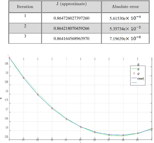
Table 3 Numerical Results of Example 3
Iteration J (approximate) Absolute error
1
0.864726027397260 5.61530e
2
0.864218070459266 5.35734e
3
0.864164568963970 7.19639e
Figure 7 Example 3 - u variables
Conclusion
An iterative method with state parameterization technique using scaling Boubaker polynomials was proved to be a good tool for evaluating the optimal solution of (QOCP) by its rapid convergence and simplicity. The numerical examples show the applicability and accuracy of this method, also comparison with other methods proves its efficiency.
References:
1.Kafash B., Delavarkhalafi A. and Karbassi S. M., Numerical Solution of Nonlinear Optimal Control Problems Based on State Parameterization, Iranian Journal of Science and Technology, Vol.A3,pp.331-340(2012).
2.Ouda E. H., The Efficient Generalized Laguerre Parameterization for Quadratic Optimal Control Problem, Journal of College of Education, Al-Mustansyriah University, vol.3, Issue (1812-0380), PP.263-276(2014).
3.Colella D. and Heil Ch., Characterizations of Scaling Functions: Continuous Solutions, SIAM Jour. of Matrix Anal. Appl., Vol. 15, No. 2, pp. 496-518, (1994).
4.Yousefi S. A., Legendre Scaling Function for Solving Generalized Emden-Fowler Equations, International Journal of Information and Systems Sciences, Vol.3,No.2,pp.243-250(2007). 5.Ouda E. H. and Ahmed I.N., Numerical Methods for Solving Optimal Control Problem Using
Scaling Boubaker Function, Al-Qadisiyah Journal of Pure Science,Vol.25,Issue(2),pp.78-89(2020).
6.Keyanpour M. and Azizsefat M., Numerical Solution of Optimal Control Problems by An Iterative Scheme, Advanced Modeling and Optimization, Vol. 13(1), (2011).
7.Ramezanpour H. et al., An Iterative Procedure for Optimal Control of Bilinear Systems, International Journal of Instrumentation and Control Systems (IJICS),Vol. 2, No.1,(2012). 8.Elaydi H. et al., An Iterative Technique for Solving Nonlinear Optimal Control Problems Using
Legendre Scaling Function, International Journal of Emerging Technology and Advanced Engineering, Vol.2,Issue (6), (2012).
9.Jaddu H. and Majdalawi A., An Iterative Technique for Solving a Class of Nonlinear Quadratic Optimal Control Problems Using Chebyshev Polynomials, International Journal of Intelligent Systems and Applications, Vol.6,pp.53-57(2014).
11.Eskandari M. J. et al., Solving the Non-linear Quadratic Optimal Control Problem in Accordance with the Standard Variational Calculus Method (VCM) and Based on Variational Iteration Method(VIM), International Journal of Review in Life Sciences,Vol.5(8),pp.1678-1686(2015). 12.Ramezani M., Numerical Solution of Optimal Control Problems by Using a New Second Kind
Chebyshev 's Wavelet, Computational Methods for Differential Equations, Vol.4,No.2,pp.162-169(2016).
13.Shihab S. N. and Delphi M. M., State Parameterization Basic Spline Functions for Trajectory Optimization , Journal of Nature, Life and Applied Sciences,Vol.3,Issue(4),pp.110-119(2019). 14.Ibraheem S. F., Ouda E. H. and Ahmed I. N., Indirect Method for Optimal Control Problem Using
Boubaker Polynomial, Baghdad Science Journal , Vol.13(1),pp.1-7, (2016).
15.Ouda E. H., A New Approach for Solving Optimal Control Problems Using Normalized Boubaker Polynomials, Emirates Journal for Engineering Research,Vol.23(4),pp.33-38(2018).
16.Vazquez-Leal H., Boubaker K., Hernandez L. and Huerta-Chua J., Approximation for Transient of Nonlinear Circuits Using RHPM and BPES Methods , Hindawi, Jour. Elect. Comp. Eng. Vol. (2013)(973813),pp.1-6.
17.Boubaker K.; On modified Boubaker polynomials: Some Differential and Analytical Properties of the New Polynomials, Journal of Trends in Applied Science Research,Vol.2,Issue(6),pp.540-544(2007).
18.Ahmed I. N. and Ouda E. H., Numerical Methods for Solving Optimal Control Problem Using Scaling Boubaker Function, Al-Qadisiyah Journal of Pure Science,Vol.25,Issue(2),pp.Math.78-89(2020).
19.Delphi M. and Shihab S., Modified Iterative Algorithm for Solving Optimal Control Problems, Open Science Journal of Statistics and Applications, Vol.6(2),pp.20-27,(2019).
20.Mehne H. H. and Borzabadi A. H., A Numerical Method for Solving Optimal Control Problems Using State Parameterization , Numer . Algor., Vol.42 , PP.165-169,(2006).