Detecting Traffic Anomalies at the Source through
aggregate analysis of packet header data
Seong Soo Kim
Department of Electrical Engineering Texas A&M University College Station, TX 77843-3128
A. L. Narasimha Reddy
Department of Electrical Engineering Texas A&M University College Station, TX 77843-3128
Marina Vannucci
Department of Statistics Texas A&M University College Station, TX 77843-3143
Abstract—The frequent attacks on network infrastructure, using various forms of denial of service attacks, have led to an increased need for developing techniques for analyzing network traffic. If efficient analysis tools were available, it could become possible to detect the attacks, anomalies and to appropriately take action to contain the attacks before they have had time to propagate across the network. In this paper, we propose a technique for traffic anomaly detection based on analyzing correlation of destination IP addresses in outgoing traffic at an egress router. This address correlation data are transformed through discrete wavelet transform for effective detection of anomalies through statistical analysis. Our techniques can be employed for postmortem and real-time analysis of outgoing network traffic at a campus edge. Results from trace-driven evaluation suggest that proposed approach could provide an effective means of detecting anomalies close to the source (campus edge). We also present data analyzing the correlation of port numbers as a means of detecting anomalies.
Keywords-Statistical analysis of network traffic; attack; anomaly; detection; wavelet transform; packet header; egress filtering; edge networks;
I. INTRODUCTION
The frequent attacks on network infrastructure, using various forms of denial of service (DoS) attacks, have led to an increased need for developing techniques for analyzing and monitoring network traffic. If efficient analysis tools were available, it could become possible to detect the attacks, anomalies and to appropriately take action to contain them before they have had much time to propagate across the network. In this paper, we study the possibilities of traffic-analysis based mechanisms for attack and anomaly detection.
The motivation for this work came from a need to reduce the likelihood that an attacker may hijack the campus machines to stage an attack on a third party. By report of Incident Response Team in 1998, 97% of the attacked sites never knew about the attacks [22]. A campus may want to prevent such use of its machines by preventing attacks, limiting misuse of its machines and possibly limiting the liability from such attacks. With this aim, we focus on analyzing network traffic at the edge of a campus. In particular, we study the utility of observing packet header data of outgoing traffic, such as destination addresses, port numbers, in order to detect attacks/anomalies originating from the campus.
Detecting anomalies/attacks close to the source allows us to limit the potential damage close to the attacking machines. Traffic monitoring close to the source may enable the network administrator quicker identification of potential anomalies and may allow better control of administrative domain’s (AD’s) resources. Attack propagation could be slowed through early detection of attacks.
Our approach monitors network traffic at regular intervals and analyzes it to find if any abnormalities are observed in the traffic. By observing the traffic and correlating it to previous samples of traffic, it may be possible to see whether the current traffic is behaving in a similar/correlated manner. The network traffic could look different because of flash crowds, changing access patterns, infrastructure problems such as router failures, and DoS attacks. In the case of bandwidth attacks, the usage of network may be increased and abnormalities may show up in traffic volume. Flash crowds could be observed through sudden increase in traffic volume to a single destination. Sudden increase of traffic on a port could signify the onset of an anomaly such as worm propagation – recent SQL Slammer worm resulted in a significant increase of traffic on port number 1434. Our approach relies on analyzing packet header data in order to provide indications of possible abnormalities in the traffic.
Our approach to detecting anomalies envisions two kinds of detection mechanisms: postmortem and real-time modes. A postmortem analysis may exploit many hours of traffic data as a single data set, employing more rigorous, resource-demanding techniques for analyzing traffic. Such an analysis may be useful for traffic engineering purposes, analysis of resource usage, understanding peak demand etc. Real-time analysis would concentrate on analyzing a small window of traffic data with a view to provide a quick and possibly dirty warning of impending/ongoing traffic anomalies. Real-time analysis may rely on less sophisticated analysis because of the resource demands and imminence of attacks.
Previous work has shown that a postmortem analysis of trace data through wavelet analysis and other techniques can reveal changes in traffic patterns [1, 3, 23]. In this paper, we also study the effectiveness of such analysis in real-time analysis of traffic data. Real-time analysis may enable us to provide means of online detection of anomalies while they are in progress. Real-time analysis may employ smaller amounts of data in order to keep such analysis simple and efficient. At the
same time, the data cannot be so small that meaningful statistical conclusions cannot be drawn. Data smoothing techniques can be employed to overcome such difficulties. However, real-time analysis may also require that any indications of attacks or anomalies be provided with short latencies. This tension between robustness and latency of anomaly detection makes real-time analysis more challenging.
The rest of the paper is organized as follows. Section II gives an overview of related work. In section III, we discuss our approach and methodology. Section IV discusses the use of address correlation as a traffic signal. Section V describes the wavelet transform of the acquired correlation signal. In section VI, we illustrate the simulation results of two kinds of detection mechanisms, more specifically postmortem and real-time analysis of the traffic signal. Section VII discusses future work, and Section VIII concludes the paper.
II. RELATEDWORK
Many approaches have been studied to detect, prevent and mitigate the malicious activities. For example, intrusion detection systems try to identify the potential DoS attack from external incoming traffic near the victims. In contrast, some approaches proactively seek a method that suppresses the overflowing of traffic at the source [5]. Controls based on rate limits have been adopted for reducing the monopolistic consumption of available bandwidth to diminish the effects of attacks, either at the source or destination [5, 7, 10, 12]. The most apparent symptoms of bandwidth attack may be sensed through monitoring bit rates [10] and packet counts of the traffic flow. Bandwidth accounting mechanisms have been suggested to identify and contain attacks [8, 9, 11, 13, 14]. Packeteer [26] and others offer commercial products that can account traffic volume along multiple dimensions and allow policy-based rate control of bandwidth. Pushback mechanisms have been proposed to contain the detected attacks closer to the source [11, 12, 27]. Traceback techniques have been proposed to trace the source of DDoS attacks even when the source addresses may be spoofed by the attacker [28].
Recently statistical analysis of aggregate traffic data has been studied [1, 3, 24]. Our previous work [1] and the work in [3] have studied traffic volume as a signal for wavelet analysis and this earlier work has considerably motivated our current study here. The work in [24] has shown the application of wavelets to network traffic data. Our study builds on this earlier work and extends the statistical analysis of traffic data further.
Traditionally, various forms of signatures have been utilized for representing the contents or certain identities. In digital information retrieval, the signature that is constructed by taking several hash values is applied for indexed representing words [17]. Traffic analysis signatures have been proposed for detecting anomalies. For example, disproportion of bi-directional flows can be used as a signature of anomalistic traffic [4]. The changing ratios (i.e., the rate of decrease) between the flow numbers of neighboring specific bit-prefix aggregate flows can be calculated and used for detecting peculiarities [6].
III. OUR APPROACH 3.1 Traffic analysis at the Source
We focus on analyzing the traffic at an egress router. A traffic monitoring at a source network enables a detector to detect attacks early and is able to control hijacking of AD (e.g., campus) machines.
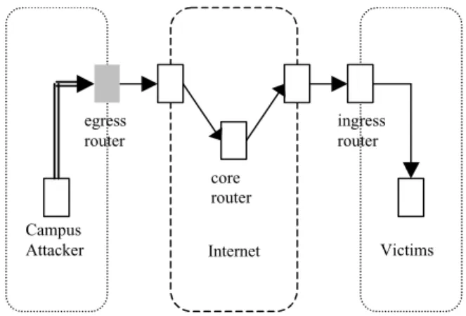
There are two kinds of filtering based on traffic controlling point. Ingress filtering protects the flow of traffic entering into an internal network under administrative control. Ingress filtering is typically performed through firewall rules to control inbound traffic originated from the public Internet. On the other hand, egress filtering controls the flow of traffic originated from internal network from being left under administrative control. Thus, internal machines are typically the origin of this outbound traffic in view of an egress filter. As a result, the filtering is performed at the campus edge [19]. Fig. 1 illustrates the various filtering points for inspection of the network traffic. Outbound filtering has been advocated for limiting the possibility of address spoofing i.e., to make sure that source addresses correspond to the designated addresses for the campus. With such filtering in place, we can focus on destination addresses and port numbers of the outgoing traffic for analysis purposes.
Our approach is based on the following observations: the outbound traffic from an AD is likely to have a strong correlation with itself over time since the individual accesses have strong correlation over time. Recent studies have shown that the traffic can have strong patterns of behavior over several timescales. For example, the traffic over a week looks very similar to the next week. Similarly, the traffic over a day exhibits a strong correlation across the next few days. It is possible to infer that some correlation exists on their weekly or daily consumption patterns. We hypothesize that the destination addresses will have a high degree of correlation for a number of reasons: (i) popular web sites, such as yahoo.com and google.com, are shown to receive a significant portion of the traffic, (ii) individual users are shown to access similar web sites over time due to their habits, and (iii) long-term flows, such as ftp download and video accesses, tend to correlate
Campus
Attacker Internet Victims
egress router ingress router core router
addresses over longer timescales. If this is the case, sudden changes in correlation of outgoing addresses can be used to detect anomalies in traffic behavior.
This hypothesis is corroborated by the data shown in Table I. The table shows the correlation of addresses across different times of day based on NZIX-II traces from NLANR (National Laboratory for Applied Network Research) [2]. The traces are sampled for 90 seconds every 3 hours and analyzed from three different viewpoints. The flows are defined by triple of destination address / destination port / protocol, and specially using 24-bit prefix destination IP address. The subject of investigation is the top 100 flows in packet counts instead of all of the flows. The packets of the top 100 flows occupy about 95% of all the packets. The first row named ‘adjacency’ shows the recurrence of destination addresses between adjacent 3-hour periods. For the 8-am column, a total of 44 addresses reappear from the previous 5-am instant. The second row titled ‘persistency’ explains the lasting continuance of addresses from the 2-am instant through the day. It is observed that 27 of the top 100 addresses persist from 2-am point to the top 100 addresses of 8-am instant. The last row titled ‘previous day’ illustrates the persistence of popular addresses in the same time points across two consecutive days. It is observed that 33 of the top 100 addresses remained the same in the 8-am instant across two different days. The correlation would be higher if we counted the traffic volume to these addresses.
3.2 General Mechanism of the detector
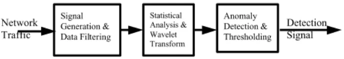
Our detection mechanisms can be explained in three major steps shown in Fig. 2. Traffic is sampled at regular intervals to obtain a signal that can be analyzed through statistical techniques and compared to historical norms to detect anomalies.
The first step is signal generation, in which the network traffic is first filtered to produce a signal that can be analyzed. So far, we have discussed how correlation of destination addresses may be used as a potential signal. The particular signal that is employed may depend on the nature of the traffic.
Fields in the packet header, such as destination addresses and port numbers, and traffic volume can be used as a signal. Packet header data, due to its discrete nature, poses interesting problems for analysis as discussed later. Sampling may be used to reduce the amount of data at this stage as explained in section IV.
The second step involves data transformation for statistical analysis. In this paper, we employ wavelet transforms to study the address and port number correlation over several timescales. Wavelet transforms have been employed to study the traffic volume earlier [1, 3]. We selectively reconstruct decomposed signal across specific timescales based on the nature of attacks. Our wavelet analysis of traffic signals is explained in section V.
The final stage is detection, in which attacks and anomalies are detected using thresholds. The analyzed information will be compared with historical thresholds of traffic to see whether the traffic’s characteristics are out of regular norms. Sudden changes in the analyzed signal are expected to indicate anomalies. This comparison will lead to some form of a detection signal that could be used to alert the network administrator of the potential anomalies in the network traffic. We report on our results employing correlation of destination addresses and port numbers as traffic signals. In this paper, we consider some statistical summary measures of the reconstructed traffic signal and apply thresholds to the sample variances, as explained in section VI.
3.3 Traces
To verify the validity of our approach, we run our algorithm on the packet traces from the NLANR. The greatest hindrance we had in using these traces is the anonymity of IP addresses. The NLANR encrypts traces out of concern for the privacy and security of those who use the network. Most of the traces did not preserve prefix relationships i.e., f(a)/p≠f(b)/p even when
a/p=b/p, wheref(a) and f(b) are the anonymized addresses of the original IP addresses a andb.
However, some long traces are sanitized by the same IP mapping database, so IP addresses identical in different traces are identical in the real world. A study of behavior of a particular machine across all the traces is thus possible. We employ University of Auckland traces of addresses collected over a campus access link for these experiments. These traces range in length from 3 days to several weeks.
3.4 Attacks
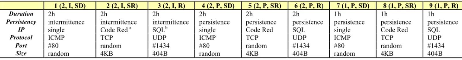
We consider nine kinds of attacks as shown in Table II. These attacks cover many kinds of behaviors and are classified by following criteria. The particular behaviors of these attacks have been motivated by recent SQL Slammer and Code Red attacks.
• Duration. The first 6 attacks continue to assail for 2 hours. The remaining 3 attacks last for 1 hour.
• Persistency. The first 3 attacks send malicious packets for 3 minutes and pause for 3 minutes. Such pattern is
TABLE I. ADDRESSPERSISTENCEINSUCCESSIVEPERIODS Sampling instances Hit ratio (%) 2-am 5-am 8-am 11-am 2-pm 5-pm 8-pm 11-pm adjacency 33 38 44 32 38 33 35 33 persistency 100 38 27 21 20 19 18 16 previous day 24 37 33 39 37 38 31 29 Network Traffic Signal Generation & Data Filtering Statistical Analysis & Wavelet Transform Anomaly Detection & Thresholding Detection Signal
repeated through the attack duration. While the filtering may mitigate the overhead of the attacker’s continuing scan traffic, a more sophisticated attacker might have stopped scanning. It may be possible to conceal attacker’s intentions through repeating attack and pause periods. So, it is intended to model intelligent and crafty attackers that attempt to dilute their trails. The other remnant attacks continue to assault throughout the attack period.
• IP address. The 1st attack among every 3 attacks targets for a single destination IP address. In a hypothetical situation, the attackers target a famous site such as The White House, CNN or Yahoo etc. This target may be really one host in case of 32-bit prefix, occasionally aggregated neighboring hosts in case of x-bit prefix. The 2nd attack style imitates from the IP address generation scheme of the notorious Code Red II worm. That is to say, a portion of addresses preserve the A and a partition of addresses preserve class-B for the infiltration efficiency. The 3rd type is
randomly generated address that was used for the Code Red I and SQL Slammer worm.
• Protocol. The 3 major protocols, ICMP, TCP and UDP, are exploited in turn.
• Port. The 2nd port among every 3 attacks target randomly generated destination ports. It is useful to detect port-scan that is used to probe a loosely defensive port. The 1st port is a representative #80 that stands for the reserved ports for well-known services. The 3rd port is a #1434 that acts for the ephemeral
client ports, which was exploited in SQL Slammer worm.
• Size. There are three different byte counts of packets. The three denominations are random size, 4KBytes and 404Bytes [19].
Our attacks can be described by a 3-tuple (duration, persistency and IP address). We superimpose these attacks on ambient traces. The mixture ratios of normal traffic and attack traffic range from 1:1 to 2:1 in packet counts. Replacement of normal traffic with attack traffic is easier to detect and hence not considered here.
IV. SIGNALGENERATION 4.1 The weighted correlation
Our approach collects packet header data at an AD’s edge over a time period, that is the sampling period. Individual fields in the packet header are then analyzed to observe anomalies in the traffic. Individual fields in the traffic header data take discrete values and show discontinuities in the sample space. For example, IP address space can span 232 possible addresses and addresses in a sample are likely to exhibit many discontinuities over this space making it harder to analyze the data over the address space. In order to overcome such discontinuities over a discrete space, we convert packet header data into a continuous signal through correlation of samples over successive samples. This signal generation phase for destination addresses is explained below.
For each address, am, in the traffic, we count the number of packets, pmn, sent in the sampling instant, sn. In order to compute address correlation signal, we consider two adjacent sampling instants. We define address correlation signal in sampling point n as
∑
∑
∗ − = m mn mpmn pmn p n C( ) 1 (1)If an address am spans the two sampling pointsn-1 andn, we will obtain a positive contribution to C(n). A popular destination address am contributes more to C(n) than an infrequently accessed destination, since we consider the number of packets being sent to different addresses.
4.2 Data structure for computing correlation
In order to minimize storage and processing complexity, we employ a simple but powerful data structure. This data structure, which is named count, consists of 4 arrays “count [4]”. Each array expresses one of the 4 fields in an IP address. Within each array, we have word-sized 256 locations, for a total of 4*256 words = 1024 words. A location count [i][j] is used to record the packet count for the addressj in ith field of the IP address. This provides a concise description of the address instead of 232locations that would be required to store the address occurrence uniquely. A similar data structure has recently been used to make the addresses more compact [4]. We filter this signal by computing a correlation of the address in two success samples, i.e., by computing
4 , 3 , 2 , 1 , ] ][ ][ [ ] 1 ][ ][ [ 255 0 − ∗ = =
∑
= counti j n counti j n i C j in (2) 1 (2, I, SD) 2 (2, I, SR) 3 (2, I, R) 4 (2, P, SD) 5 (2, P, SR) 6 (2, P, R) 7 (1, P, SD) 8 (1, P, SR) 9 (1, P, R) Duration 2h 2h 2h 2h 2h 2h 1h 1h 1hPersistency intermittence intermittence intermittence persistence persistence persistence persistence persistence persistence
IP single Code Red a SQLb single Code Red SQL single Code Red SQL
Protocol ICMP TCP UDP ICMP TCP UDP ICMP TCP UDP
Port #80 random #1434 #80 random #1434 #80 random #1434
Size random 4KB 404B random 4KB 404B random 4KB 404B
a. semi-random
b. random
Fig. 3 depicts the data structure that consists of the 2-dimensional array count[i][j]. The 1st dimension array
corresponds the 4 byte segments of the IP address (separated by a dot in the normal IP address representation), and is represented to be 4 rows in the data structure. The 2nd dimension indicates the 256 entries of each IP address segment, and is expressed as the 256 columns in each row.
We illustrate this data structure through an example. Suppose that only five flows exist, their destination IP addresses and packet counts are as follows.
IP of F1 = 165. 91. 212. 255, P1= 3 IP of F2 = 64. 58. 179. 230, P2= 2 IP of F3 = 216. 239. 51. 100, P3= 1 IP of F4 = 211. 40. 179. 102, P4= 10 IP of F5 = 203. 255. 98. 2, P5= 2
All components in the count arrays are initialized to zeros. The packet counts of each flow are recorded to the corresponding position of each IP address segment as shown in Fig. 3.
In order to compute the correlation signal at the end of sampling point n, we simply multiply values in the same position between the two data structures of samplesn-1 and n, then sum up the multiplied values in each segment separately. Consequently four correlation signals are calculated as C1n through C4n. The employment of this approximate representation of addresses allows us to reduce the computational and storage demands by a factor of 222.
In order to generate the address correlation signalS(n) at the end of sampling point n, we multiply each segment correlation Cin with scaling factors αi and generate S(n) as
B C C C C A n S( )= ∗(α1∗ 1n+α2∗ 2n+α3∗ 3n+α4∗ 4n)+ 1 ,α1+α2+α3+α4= where (3)
This data structure has following advantages.
• The running time of the signal generation diminishes from O(n) to O(lgn).
• It is possible to track the target IP addresses. By assembling the highest valued position in each of the 4 fields, specific attack objectives can be drawn. In Fig. 3, we can get the 211.40.179.102 as IP of F4 when the
positions of highest value in each field combine together.
By properly choosing the scaling factors, we can obtain appropriate aggregation of address space. In this paper, we employ α1 = α2 = α3 = α4 = 1/4. On the other hand, we could
employ different weights to give preferences to different portions of the address segments. For example, by making C3n =C4n = 0, we only consider /16 addresses.
Our approach could introduce errors when the addresses segments match even though addresses themselves don’t match. For example, if traffic consists of w1.x1.y1.z1 and
w2.x2.y2.z2in sample n-1 and w1.x1.y2.z1 and w2.x2.y1.z2in sample
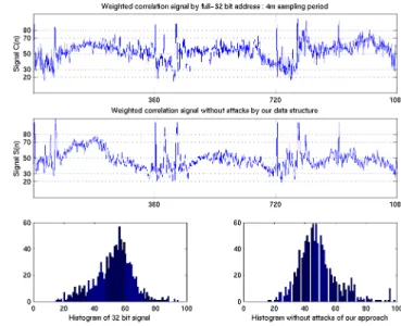
n, even though the actual address correlation is zero, our method of computing address correlation results in a high correlation between these sampling instants. In normal traffic without attacks, we compared the full-32 bit address correlation with the correlation signal generated by our approach. Fig. 4 shows the weighted signal computed with the full-32 bit address correlation and our data structure. From the figure, we see that the differences are negligible i.e., our approach does not add significant noise. From a statistical point of view, they have an approximately same mean (about 50) and degree of dispersion (standard deviation ≅ 12.4 ~ 12.6).
4.3 The signal distribution in ambient traces
The second sub-picture in Fig. 4 depicts the weighted correlation signal, S(n), that is calculated through the above procedure in 3-day traces without attacks. The traces are sampled for 60 seconds every 4 minutes. This signal is scaled to center around 50 and mostly fluctuates between 70 and 30 considering some exceptions. The right-bottom sub-picture shows the histogram of this signal in graphic. This signal fails to pass the null hypothesis that samples are distributed normally. Their statistical characteristic is that the mean is approximately 50, and standard deviation is 12.4 as Table III Fri/Sun row indicates. This weighted correlation signal itself may be used to detect anomalies as a coarse method. It can be
0 64 128 192 255
2 3 2 10 1
10 2 3 1 2 1 2 12 3
2 1 10 2 3
Figure 3. Data structure for computing weighted correlation
done through employing three levels of threshold.
a) Green zone: We can define green zone as the interval
including 90% of data around mean of the correlation values of IP address. Roughly this zone is between 30 and 70. This zone could be considered as the normal state.
b) Red zone: Red zone is defined as the interval
including 2% outlier data from either end of the values. Roughly this zone is below 20 and over 80. This zone may indicate anomalies.
c) Yellow zone: It includes the data between the green
zone and the red zone indicating possible anomalies or infrequently occurring traffic patterns.
And this second sub-picture in Fig. 4 shows the occurrence of some peaks that may be flash crowds or peak noise. These noises degrade the detector by inducing type I errors.
4.4 The signal distribution with attacks
The second sub-picture in Fig. 5 represents the weighted correlation signal of IP address in 3-day traces with attacks. The simulated attacks are staged between the vertical lines, shown in the figure. Almost all of the attacks reach the yellow
or red zone. The first 3 attacks described in (*,I,*) show an oscillation because of their intermittent nature, while the remaining six attacks described in (*,P,*) give a rectangular-shaped signal because of their persistence. The 1st attack among every 3 attacks, that is (*,*,SD), indicate very high correlation because of their single destination IP address, on the other hand, the remnants show a very low value because of their randomness. The 3rd attack, (*,*,R), shows lower value than 2nd attack, (*,*,SR), due to pureness. The 1st through 6th attack
which can be represented in (2,*,*) last for 2 hours, and the rests, namely (1,*,*), maintain for 1 hour.
This sub-picture still shows the occurrence of some peak noises that can give rise to false positives. These side effects weaken the detection performance, so we still more need to filter these noises out for better detection.
V. DATATRANSFORM
5.1 Data Transform
The generated signal can be, in general, analyzed by employing techniques such as FFT (Fast Fourier Transform) and wavelet transforms. The analysis carried out on the signal may exploit the statistical properties of the signal such as correlation over several timescales and its distribution properties. FFT of traffic arrivals may reveal inherent flow level information through frequency analysis. Wavelet transform of traffic traces has been employed in [1], [3]. We employ wavelet transforms, in this paper, for analyzing the traffic signal.
Wavelet techniques are one of the most up-to-date modeling tools to exploit both non-stationary and long-range dependence [20, 21, 22]. Wavelet analysis can reveal scaling properties of the temporal and frequency dynamics. We compute a wavelet transform of the generated address correlation signal over several sampling points.
5.2 Discrete Wavelet transform
We provide a brief overview of DWT (Discrete Wavelet Transform) in order to make our scheme clearer. DWT consists of decomposition (or analysis) and reconstruction(or synthesis).
Figure 5. Comparison of signal distribution without attacks and with attacks
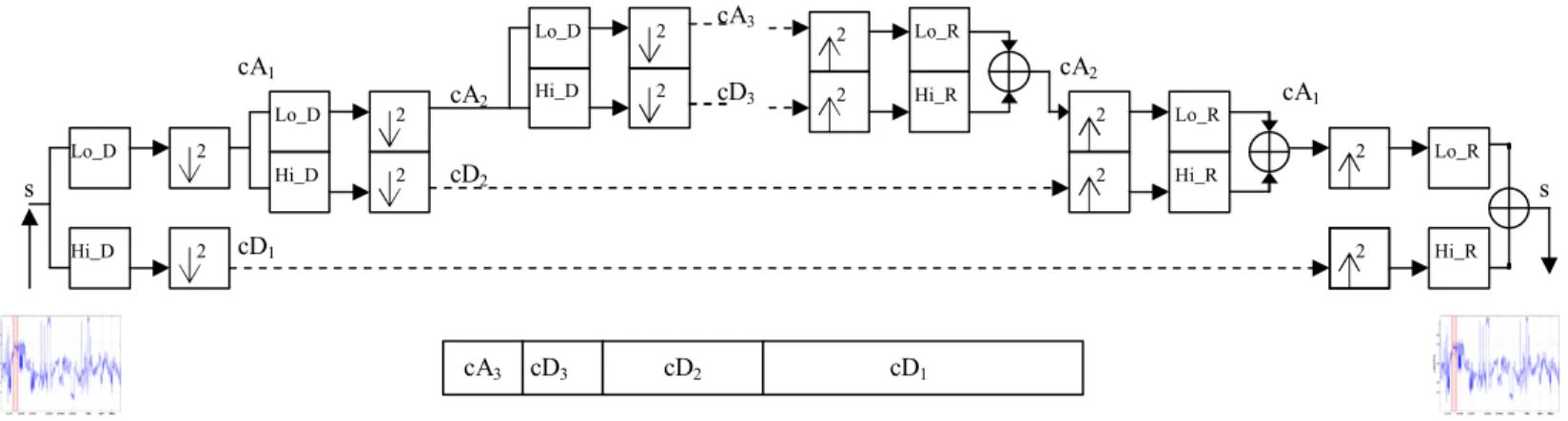
s s cA3 Lo_D Hi_D 2 2 cD1 cA1 Lo_D Hi_D 2 2 Lo_D Hi_D 2 2 cD2 cA2 cD3 Lo_R Hi_R 2 Lo_R Hi_R 2 2 Lo_R Hi_R 2 2 2 cD3 cA3 cD2 cD1
Figure 6. A Multilevel two-band wavelet decomposition and reconstruction cA2
Fig. 6 illustrates a multilevel one-dimensional wavelet analysis using specific wavelet decomposition filters (Lo_D and Hi_D are the low-pass and high-pass decomposition filters) and the reconstruction of the original signal [18].
For decomposition, starting from a signal s, the first step of the transform decomposes s into two sets of coefficients, namely approximation coefficients cA1, and detail coefficients
cD1. The input s is convolved with the low-pass filter Lo_D to
yield the approximation coefficients. The detail coefficients are obtained by convolving s with the high-pass filter Hi_D. This procedure is followed by down sampling by 2. Suppose that the length of each filter is equal toN. If n = length(s), the each convolved signal is of length n + N- 1 and the coefficients cA1 and cD1 are of length L =floor((n+N-1)/2). The second
step decomposes the approximation coefficient cA1 into two
sets of coefficients using the same method, substituting s by cA1, and producing cA2 and cD2, and so forth. At levelj, the
wavelet analysis of the signals has the following coefficients, [cAj, cDj, cDj-1, cDj-2, ... , cD2, cD1].
For reconstruction, starting from two sets of coefficients at level j, that is the approximation coefficients cAj and detail
coefficients cDj, the inverse DWT synthesizes cAj-1,
up-samples by inserting zeros and convolves the up-sampled result with the reconstruction filters Lo_R and Hi_R. Let L be the length of cA and cD, andN be the length of the filters Lo_R and Hi_R, then length(s) = 2*L-N+2. For a discrete signal of lengthn, DWT can consist of log2n levels at most.
5.2.1 Timescales selection
We iterate analysis level up to 8, so our final analysis coefficients are [cA8, cD8, cD7, cD6, cD5, cD4, cD3, cD2, cD1].
We employ a daubechies-6 two-band filter. If we use all coefficients for reconstruction, we would get the original weighted correlation signal. The filtered signal is down-sampled by 2 at each level of the analysis procedure; the signal of each level has an effect that sampling interval extends 2 times. Consequently it means that the wavelet transform identifies the changes in the signal over several timescales. When we uset minutes as sampling interval, the time range at levelj spans t*2j minutes. For instance, when we use 4-minute sampling interval, the cD1equals to 4*21 = 8 minutes, the cD2
equals 4*22 = 16 minute interval and so on. 5.3 Selective reconstruction
We simulate two classes of attacks based on persistence, namely the first 3 attacks are ON/OFF styled attacks and remaining six attacks are persistent attacks. These two categories are easily differentiated by the attribute of signal. These heterogeneous attacks could be effectively detected when the appropriate analyzed level of the original signal is selectively used for synthesis. Because of the time-scale decomposition of the wavelets we are able to detect changes in the behavior of the network traffic that may appear at some resolution but go un-noticed at others.
The first three attacks described in (*,I,*) have an ON/OFF timing of 3 minutes, so they have a period of 6 minutes. This signal could be effectively detected by only the 1st coefficient of the DWT. Detection results of first 3 attacks using cD1
coefficient in postmortem and real-time mode are shown in Fig. 7(a). The attacks assail between the vertical lines, and the detection signal is shown with dots at the bottom of the each sub-picture. When the system administrator concentrates on 30-minute duration signal, he/she can select a higher level coefficient (for example 3, cD3), for detecting designated
attacks instead of cD1.
The last six attacks expressed in (*,P,*) are persistent attacks. Attacks last for 1 hour at a minimum. It means that we could choose the cD4, cD5 and cD6 levels among all the
coefficients for reconstruction that are equivalent to 1 hour 4 minutes, 2 hour 8 minutes and 4 hour 16 minutes respectively, in the case of 4-minute sampling interval. Detection results of latter six attacks using cD4to cD6coefficients in both modes are
(a) Selective DWT 1: cD1 reconstructed signal-based detection results
(b) Selective DWT 2: cD4,cD5,cD6 reconstruction based detection results
shown in Fig. 7(b). It is observed that the address correlation signal and subsequent wavelet analysis has provided a mechanism for detecting these attacks.
To demonstrate the feasibility of our composite approach, we focus the evaluation of our scheme over the 9 types of attacks discussed earlier. In order to detect these attacks, we extract only the 1st, 4th, 5th and 6th levels in decomposition and reconstruct the signal based only on coefficients at these levels. We choose coefficients for reconstruction based on the length of the attacks. In reality, because the length of the attack and the nature of attack may be unknown, we should design a general-purpose mechanism. There can be many possible approaches. We outline one such potential approach. At normal times, the detector checks only the reconstructed signal based on lower level coefficients (say, the 1st level), which can identify the most detailed and instantaneous change in the traffic signal. Once suspicious abnormal sign is detected, detector expands its investigative scope into higher level gradually. It may help to reveal the substance of attack and to diminish the false alarm under unknown conditions. We present preliminary results of such an approach in section 6.6. Our intent here is to demonstrate the feasibility of detecting potential attacks and anomalies by analyzing traffic header data.
VI. DETECTION
6.1 Thresholds setting through statistical analysis
We develop a theoretical basis for deriving thresholds for anomaly detection. If we assume that the reconstructed signal has a normal distribution, we can design suitable analysis and detection techniques to detect anomalies with high confidence while reducing the false acceptances.
To verify our methodology, we select only some levels of the DWT decomposition of the ambient trace without attacks and reconstruct the signal based on those levels. We then look at some statistical properties. The center sub-picture in Fig. 8 shows the histogram of the reconstructed signal of the ambient traces in postmortem mode. The postmortem transformed data without attacks have mean 0 and standard deviation 3.4. We verify normality of the Fri/Sun data in Table III through the Lilliefors test. The postmortem transformed data have a normal distribution at 5% significance level, namely X~N(0, 3.42). The original weighted correlation data fail to pass the null hypothesis of normality, however, the DWT converts it to normal distribution. By selecting some of the levels, we have removed some of the features from the signal that were responsible for the non-normality in the original signal. When
we set the thresholds to –9 and 10 respectively, these figures are equivalent to –2.6σ < X < 3σ confidence interval. This interval corresponds to 99.4% confidence level. With such thresholds, we can detect attacks with error rate of 0.6%.
We also analyze the reconstructed signal at our selected levels of ambient trace in real-time mode, which show approximately normal distribution. The right sub-picture in Fig. 8 shows the histogram of the reconstructed signal of the ambient traces in real-time mode.
6.1.1. Statistical consideration of thresholds
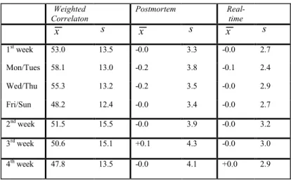
If statistical parameters of network traffic, such as mean and standard deviation, are similarly distributed given different days, parameters of specific day could be applied to other days. We gather the 4-week traces and analyze their statistical summary measures. Table III shows the distribution in other days. Let’s suppose we know only the 1st week data and use the three-sigma limits. The thresholds for real-time detection are
1 . 8
± at 99.7% confidence level. When the very same thresholds are applied in 2nd week traffic, they equal to
s
53 . 2
± at 99% level. It illustrates that the thresholds could remain approximately the same over several days.
6.2. Real-time detection mechanism
The reconstructed signal is used for detecting anomalies. The post-mortem analysis and detectors can rely on datasets over long periods of time. However, real-time detection requires that the analysis and the detection mechanism rely on small datasets in order to keep such online analysis feasible. As explained earlier, smaller datasets raise the possibility of many false alarms. Larger datasets may increase the latency of detection even when online analysis of such datasets is feasible. We took the following approach to accommodate faster detection while reducing the false alarms.
At each sampling instance, we construct the correlation signal S(n). We consider p samples, S(n-p+1), S(n-p+2),…, S(n-1) and S(n) for the computation of DWT at the sampling point n. We call p, the analysis (DWT) window. And we
Figure 8. Various histograms of the ambient traces without attacks
TABLE III. THESTATISTICALPARAMETER IN DIFFERENTDAYS Weighted Correlaton Postmortem Real-time x s x s x s 1st week 53.0 13.5 -0.0 3.3 -0.0 2.7 Mon/Tues 58.1 13.0 -0.2 3.8 -0.1 2.4 Wed/Thu 55.3 13.2 -0.2 3.5 -0.0 2.9 Fri/Sun 48.2 12.4 -0.0 3.4 -0.0 2.7 2nd week 51.5 15.5 -0.0 3.9 -0.0 3.2 3rd week 50.6 15.1 +0.1 4.3 -0.0 3.0 4th week 47.8 13.5 -0.0 4.1 +0.0 2.9
considerq (≤p) samples, S(n-q+1), S(n-q+2),…, S(n-1), and S(n) for anomaly detection. We call q, the detection (DET)
window. To reduce false alarms due to instant noise, we use a
majority over the detection window to detect anomalies. If q/2
or more of the samples in the detection window are above the anomaly threshold, we consider that an anomaly is detected at the sampling point n. This majority detector requires that traffic exhibit anomalous behavior over several sampling points (at leastq/2 in a window of q samples) for a successful detection. When q is large, we can keep false alarms low. However, largerq also increases latency of anomaly detection since such a majority function delays the attack detection for at least q/2
sampling periods. As a result, attacks smaller thanq/2 sampling periods are likely to be not detected. We illustrate these observations in Fig. 9.
Based on Fig. 9, the detectable attack duration time is the half of the detection widow width at least when m is ½. Detection indication signal, T, expands from mW to D+(1-m)W. According to selected m value, the period of T is changeable between |W-D| and W+D. Therefore the latency of detection is mW. The empirical results, however, show the variable latency depending on the attack strength and threshold level.
6.3 Detection anomalies using thresholding
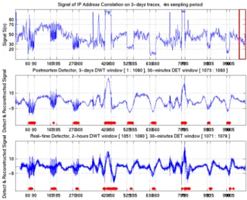
Detection results of our composite approach are shown in Fig. 10. The top-most sub-picture illustrates a weighted correlation signal of IP addresses that is used for wavelet transform with attacks. The second sub-picture is the wavelet-transformed and reconstructed signal in postmortem and its detection results. The last sub-picture shows the wavelet-transformed and reconstructed signal in real-time and its accumulated results.
We employ 3-day traces of addresses collected over a campus access link for these experiments. A sampling interval
is 4 minutes and a sampling duration is 60 seconds. That is to say, we sampled for 1 minute and paused for 3 minutes and so on. The simulated nine attacks are staged between the vertical lines, shown in the figure. The detection signal is shown with dots at the bottom of the each sub-picture. Overall, our results show that our approach may provide a good detector of attacks in both modes. Let’s discuss the detection results in both modes in detail.
6.3.1 Discussion of Postmortem analysis
The postmortem analysis uses whole 3-day correlation data all at once. To evaluate the reconstructed signal we use –9 and 10 as statistical threshold in second sub-picture of Fig 10. The reconstructed signals of first 3 attacks (*,I,*) show an oscillatory fashion because of their intermittent attack patterns, while the remaining six attacks, namely (*,P,*), give a shape of hill and dale at attack times due to persistence.
The attacks on a single machine, more specially the 1st attack among every 3 attacks described in (*,*,SD), reveal the high valued correlation which means the current traffic is concentrated on (aggregated) a single destination. Detection signals in the form of dots show that these typed attacks can be detected effectively. On the other hand, the semi-random typed attacks, that is (*,*,SR), and random styled attacks, namely (*,*,R), illustrate low correlations which means traffic is behaving in irregular pattern. These attacks can be also captured across attack time. Consecutive detection signals indicate the length of attacks and also imply the strength of anomalies.
6.3.2 Discussion of Real-time analysis
The online analysis only exploits a short span of recent correlation data. The most recent 2-hour correlation data make use of detecting an attack at given point of sampling. It is implemented with a 2-hour wide DWT window, which is shown as rectangle in the right corner of topmost sub-picture in Fig. 10. The 2-hour width is selected as a trade-off between prompt response and robustness. We employed a detection
D W mW latency W mW (1-m)W T where,
D is the attack duration in reconstructed signal
W is detection (DET) window size (=qt,t is sampling interval) T is maximum indication time
m is the majority factor for decision (=1/2)
Figure 9. The detection timing diagram in real-time mode
(DET) window of 8 sampling periods, which is 30 minutes. As the bottom-most picture in Fig. 10 shows, however, our detector achieves acceptable attack detection performance in online analysis as well as in offline analysis.
Although the latter 3 attacks described in (1,*,*) probe for a short period of time at low rate comparison to the first 6 attacks, our detector do not depend on the duration and rate of attacks.
Table IV shows the overall timing relationship between detection latency and the setting of the confidence level of our simulated attacks in real-time mode. As we expect, the higher the confidence level, the higher the detection latency. When the confidence level is low, many false alarms are incurred because of imprudence of detection; on the other hand, almost all of the attacks can be detected without false negatives. As the threshold is increased, the false acceptance is diminished, however, the false rejection is induced sometimes. The detection against the (*,*,SD) typed attacks, (aggregated) single destination, can achieve a prompt response. And the (*,*,R) typed attacks, randomly generated destination, can generally be detected more quickly than the semi-random type attacks described in (*,*,SR) because of the resulting lower correlation with random attacks. Even though, our real-time
analysis results are promising that attacks may be detected in a few minutes, recent studies [25] indicate that worm propagation control measures need to react even faster to be effective. In the future, we plan to develop techniques for swifter identification of these attacks.
6.4 Analysis of network traffic by Port numbers
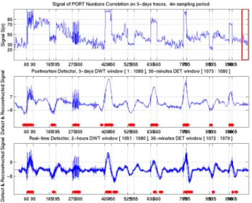
It seems feasible to carry out a similar correlation and wavelet-based analysis of network packets based on their port numbers. This is particularly motivated by the recent large-scale attacks Code Red and SQL Slammer. Both attacks have been spawned on particular ports exploiting unique weaknesses of end applications. It has been observed that in both cases, an unusually large number of packets were generated on these ports during the attack. We simulate the attacks in Table II, and repeat the same procedure as earlier, but now with port numbers as the traffic signal.
Our correlation-based analysis shows marked variations during an attack when we consider port numbers of packets as data. Detection results of our approach are shown in Fig. 11.
The top-most sub-picture illustrates a weighted correlation signal of port numbers that are used for wavelet transform. The second sub-picture shows the wavelet-transformed signal in postmortem analysis and its detection results. The transformed data without attack, which shows approximately normal distribution, have 0 as mean and 3.0 as standard deviation. The –9 and 7 values as thresholds equivalent to –3σ < X < 2.3σ confidence interval. They correspond to 98.8% confidence level. The last sub-picture shows the wavelet-transformed signal in real-time analysis and its results. The results indicate that correlation of port numbers over samples of network traffic could provide a reliable signal for analyzing and detecting traffic anomalies. When attacks are staged on a particular port, we find high correlation and when attacks are staged on random ports, we find the correlation to be low.
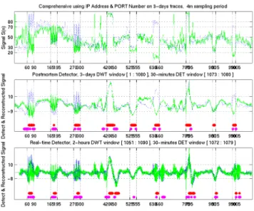
6.5 Comprehensive traffic anaysis
Up to now, our work has shown that analysis of addresses and port numbers may individually provide indicators of traffic anomalies. Is it possible to combine several indicators to build a more robust anomaly detector that is less prone to false alarms? Fig. 12 shows the comprehensive anomaly detector based on a combination of addresses and port numbers.
confidence level 1 (2, I, SD) 2 (2, I, SR) 3 (2, I, R) 4 (2, P, SD) 5 (2, P, SR) 6 (2, P, R) 7 (1, P, SD) 8 (1, P, SR) 9 (1, P, R) false positive false negative 1.0s 68 % 0a 4 6 0 2 2 0 6 0 10 0 1.5s 86 % 8 6 8 0 10 10 0 18 6 9 0 2.0s 95.5 % 10 8 12 0 26 22 0 28 26 7 0 2.5s 98.5 % 12 8 12 0 38 28 0 36 32 7 0 setting 99.5 % 12 12 18 0 40 32 0 38 36 3 0 3.0s 99.7 % 16 12 36 0 54 42 0 44 38 3 0 3.5s 99.95 % 22 12 42 0 Xb 66 4 X 60 3 2 4.0s 99.99 % 22 42 X 2 X X 4 X X 1 5
a. Latency is measured by minute unit
b. X means non-detection
TABLE IV. THERELATION BETWEEN LATENCIES AND CONFIDENCELEVELS IN NINEKINDS OF ATTACKS IN REAL-TIME MODE
The two kinds of dots at the bottom of each sub-picture show detection results. The dots located on top are marked when both the address and port methods detect anomalies simultaneously. The dots located on the bottom are displayed when only one of the two detection methods detects anomalies. It can be understood that the above markings imply very high confidence and the lower dots imply probable detections.
6.6 Adaptive filtering
In order to detect anomalies of different unknown durations, we considered adaptive filtering of the traffic signal. Adaptive filtering continues to search for the proper levels of timescales suitable to the nature of the attack. At normal times, the detector monitors only the reconstructed signal based on aggregated 1, 2 and 3 levels. Once a possible detection of anomaly is identified at these levels, the detector considers signal at higher levels, for example at levels 2, 3 and 4, for improving the identification accuracy or robustness. False alarms can be reduced by not declaring the detection of an anomaly until consecutive alarms are raised at multiple levels. The traffic signal at higher levels is considered as the identification progresses. On the other hand, if an anomaly is not detected, the reconstructed signals return to lower levels gradually. The Table V shows the preliminary results of such an approach. The table shows the real-time detection latency based on a 2-minute sampling period and a 10-minute detection window over a 3-day trace. The results indicate that it may be feasible to detect traffic anomalies with low latency even when we consider attacks of unknown length.
VII. FUTURE WORK
The duration of the samples and the number of samples have a strong impact on the accuracy of the results and the latency for detecting an attack. For example, when we employ a sampling interval of 10 minutes, each sample is likely to be more stable and less noisy than with a smaller sampling period, of say 1 minute. The noisier sample leads to more false positives since a smaller number of changes in the network traffic are sufficient to cause significant changes in the filtered signal. However, the samples with a smaller sampling period lead to faster identification of the attack. It is a pivotal factor for the real-time approach we discussed. Thus, as a further research, the relation between sampling rate and latency should be investigated from statistical point of view.
We plan to build a robust multidimensional tool that analyzes addresses, port numbers, traffic volume and other data for the detection of anomalies over several timescales. We plan to study containment approaches along the multiple dimensions of addresses, port numbers, protocols and other such header data (through rate throttling) based on such a detection tool. We also plan to study the effectiveness of the analysis of traffic header data at various points in the network, at the destination network (as opposed to the source network that is considered in this paper) and within the network core. For example, reflection attacks may employ machines outside the campus and hence may not enable observation of changes in traffic at the edge of the campus.
VIII. CONCULSION
We studied the feasibility of analyzing packet header data through wavelet analysis for detecting traffic anomalies. Specifically, we proposed the use of correlation of destination IP addresses and port numbers in the outgoing traffic at an egress router. Our results show that statistical analysis of aggregate traffic header data may provide an effective mechanism for the detection of anomalies within a campus or edge network. We studied the effectiveness of our approach in postmortem and real-time analysis of network traffic. The results of our analysis are encouraging and point to a number of interesting directions for future research.
ACKNOWLEDGMENT
We are very grateful to Deukwoo Kwon for his comments and reviews on statistical analysis, to David Cheney and Joerg B. Micheel at NLANR for their comments about trace information, to David Moore at CAIDA for his help in accessing traces. In addition, we would like to thank Hyoseon Kim for his helpful suggestions and comments on this paper.
REFERENCES
[1] Anu Ramanathan, “WADeS: A Tool for Distributed Denial of Service Attack Detection”, TAMU-ECE-2002-02, Master of Science Thesis, August 2002.
http://dropzone.tamu.edu/techpubs/2002/thesis_ramanathan.pdf [2] National Laboratory for Applied Network Research (NLANR),
measurement and operations analysis team, “NLANR network traffic packet header traces”, accessed in August 2002.
http://pma.nlanr.net/Traces/ Figure 12. The comprehensive detection results
confidence level 1 2 3 4 5 6 7 8 9 false alarm false negative setting 99.5 % 2a 8 10 4 6 6 0 6 4 5 0
a. Latency is measured in minutes.
[3] P. Barford, J. Kline, D. Plonka and A. Ron, “A Signal Analysis of Network Traffic Anomalies,” in Proceedings of ACM SIGCOMM Internet Measurement Workshop, Marseille, France, November 2002. [4] Thomer M. Gil and Massimiliano Poletto, “MULTOPS: A
Data-Structure for Bandwidth Attack Detection”, inProceedings of the 10th
USENIX Security Symposium, Washington, D.C., USA, August 2001.
[5] J. Mirkovic, G. Prier and P. Reiher, “Attacking DDoS at the Source”, in 10th IEEE International Conference on Network Protocols
, Paris, France, November 2002.
[6] E. Kohler, J. Li, V. Paxson and S. Shenker, “Observed Structure of Addresses in IP Traffic, in Proceedings of ACM SIGCOMM Internet
Measurement Workshop, Marseille, France, November 2002.
[7] A. Garg and A. L. Narasimha Reddy, "Mitigation of DoS attacks through QoS regulation", in Proc. of IWQOS workshop, May 2002. [8] Smitha, Inkoo Kim and A. L. Narasimha Reddy, "Identifying long term
high rate flows at a router", inProc. of High Performance Computing, December 2001.
[9] Inkoo Kim, “Analyzing Network Traces To Identify Long-Term High Rate Flows”, TAMU-ECE-2001-02, Master of Science Thesis, May 2001.
http://dropzone.tamu.edu/techpubs/2001/thesis_ben9.pdf
[10] Yin Zhang, Lee Breslau, Vern Paxson and Scott Shenker,”On the Characteristics and Origins of Internet Flow Rates”, in ACM SIGCOMM 2002, Pittsburgh, PA, USA, August 2002.
[11] Ratul Mahajan, Steven M. Bellovin, Sally Floyd, John Ioannidis, Vern Paxson and Scott Shenker, “Controlling High Bandwidth Aggregates in the Network (Extended Version)”, in ACM SIGCOMM Computer Communication Review, Volume 32 , Issue 3, July 2002.
[12] John Ioannidis Steven M. Bellovin, “Implementing Pushback: Router-Based Defense Against DDoS Attacks”, in Proceedings of Network and Distributed System Security Symposium, San Diego, California, February 2002.
[13] Christian Estan and George Varghese, “New Directions in Traffic Measurement and Accounting”, inACM SIGCOMM 2002, Pittsburgh, PA, USA, August 2002.
[14] A. Medina, N. Taft, K. Salamatian, S. Bhattacharyya and C. Diot, “Traffic Matrix Estimation: Existing Techniques and New Directions”,
inACM SIGCOMM 2002, Pittsburgh, PA, USA, August 2002.
[15] Kimberly C. Claffy, Hans-Werner Braun, George C. Polyzos, “A parameterizable methodology for Internet traffic flow profiling”, in IEEE Journal on Selected Areas in Communications, Oct. 1995, vol.13, (no.8):1481-94.
[16] C. S. Burrus, R. A. Gopinath and H. Guo, Introduction to Wavelets and Wavelet Transforms, Prentice Hall, 1998.
[17] I. H. Witten, A.Moffat and T. C. Bell, Managing Gigabytes – Compressing and Indexing Documents and Images, 2nd ed., Morgan Kaufmann, 1999, pp.129–141.
[18] The MathWorks. Inc., MatLab software, ver 6.1.0.450 Release 12.1, May 2001.
[19] CERT Coordination Center (CERT/CC), “CERT Advisory CA-2003-04 MS-SQL Server Worm”, January 2003.
http://www.cert.org/advisories/CA-2003-04.html
[20] Daubechie I., “Ten lectures on wavelets”, Volume 61 of CBMS-NSF Regional Conference Series in Applied Mathematics, Philadelphia: Society for Industrial and Applied Mathematics, 1992.
[21] Mallat S., "A theory for multiresolution signal decomposition: the wavelet representation", IEEE Transactions on Pattern Analysis and Machine Intelligence, vol. 11, no. 7, pp 674-693, 1989
[22] Wornell G. W., Signal Processing with Fractals: A Waveleyt Based Approach, New Jersey: Prentice Hall, 1996
[23] Ellen Mitchell, “Introduction to Computer Security”, in Proceedings of Texas Workshop on Security of Information Systems, College Station, USA, April 2003,
http://net.tamu.edu/~ellenm/papers/ics.ppt
[24] Anja Feldman, Anna Gilbert, Polly Huang and Walter Willinger, “Dynamics of IP traffic: A study of the role of variability and the impact
of control”,Computer Communication Review, Vol. 29, No. 4 (Proc. of
the ACM Sigcomm'99, Cambridge, MA), pp. 301-313, 1999.
[25] David Moore, Colleen Shannon, Geoffrey M. Voelker, and Stefan Savage, “Internet Quarantine: Requirements for Containing Self-Propagating Code”, in INFOCOM 2003 conference, April, 2003. [26] Packeteer, “PacketShaper Express”, white paper, 2003.
http://www.packeteer.com/resources/prod-sol/Xpress_Whitepaper.pdf [27] Sally Floyd, Steve Bellovin, John Ioannidis, Kireeti Kompella, Ratul
Mahajan and Vern Paxson, “Pushback messages for controlling aggregates in the network”, IETF RFC, July 2001.
[28] Stefan Savage, David Whetherall, Anna Karlin and Tom Anderson, “Practical network support for IP traceback”,Proc. of ACM Sigcomm, 2000.
![Fig. 6 illustrates a multilevel one-dimensional wavelet analysis using specific wavelet decomposition filters (Lo_D and Hi_D are the low-pass and high-pass decomposition filters) and the reconstruction of the original signal [18]](https://thumb-us.123doks.com/thumbv2/123dok_us/9085553.2400431/7.918.506.871.342.633/illustrates-multilevel-dimensional-analysis-specific-decomposition-decomposition-reconstruction.webp)