The Oceanographic Multipurpose Software
Environment
Inti Pelupessy
1,2, Ben van Werkhoven
3, Arjen van Elteren
2, Jan Viebahn
1,
Adam Candy
4, Simon Portegies Zwart
2, and Henk Dijkstra
11Institute for Marine and Atmospheric Research Utrecht, Utrecht University, The Netherlands. 2Leiden Observatory, Leiden University, The Netherlands
3The Netherlands eScience Center, The Netherlands
4Civil Engineering and Geosciences, Delft Technical University, The Netherlands Correspondence to:Inti Pelupessy ([email protected])
Abstract.
In this paper we present the Oceanographic Multipurpose Software Environment (OMUSE). This framework aims to provide a homogeneous environment for existing or newly developed numeri-cal ocean simulation codes, simplifying their use and deployment. In this way,OMUSEfacilitates the design of numerical experiments that combine ocean models representing different physics or 5
spanning different ranges of physical scales. Rapid development of simulation models is made pos-sible through the creation of simple high-level scripts, with the low-level core part of the abstrac-tion designed to deploy these simulaabstrac-tions efficiently on heterogeneous high performance comput-ing resources. Cross-verification of simulation models with different codes and numerical methods is facilitated by the unified interface thatOMUSEprovides. Reproducibility in numerical experi-10
ments is fostered by allowing complex numerical experiments to be expressed in portable scripts that conform to a commonOMUSEinterface. Here, we present the design ofOMUSEas well as the modules and model components currently included, which range from a simple conceptual quasi-geostrophic solver, to the global circulation modelPOP. We discuss the types of the couplings that can be implemented usingOMUSEand present example applications, that demonstrate the efficient 15
and relatively straightforward model initialisation and coupling withinOMUSE. These also include the concurrent use of data analysis tools on a running model. We also give examples of multi-scale and multi-physics simulations by embedding a regional ocean model into a global ocean model, and in coupling a surface wave propagation model with a coastal circulation model.
1 Introduction 20
Models of the global open ocean have now reached a mature state. Different models, such asMITgcm,
MPI-OM,POP,MOM,NEMO, which have been developed in large international collaborations, are
CMIP5-type global climate models, with a horizontal resolution as fine as 25 km, focusing on projected forecasts of future climate change (IPCC, 2013). They are also used in an ocean-only model con-25
figuration (Maltrud et al., 2010) at even higher resolutions (down to about 10 km) to adequately resolve western boundary currents, such as the Gulf Stream, the Agulhas Current and Kuroshio, and to explicitly represent meso-scale eddies.
At the coastal zone, very different models are required, incorporating, for example, tides, river run-off, sediment transport and wave dynamics (e.g. Zijlema, 2010). In many cases, unstructured 30
mesh models are used (Danilov, 2013; Leuttich and Westerink, 2004) in order to provide an accurate representation (Candy et al., 2014) of complex and irregular domain bounds that strongly influence local flows. An additional challenge in regional coastal ocean models, such asADCIRCandSWAN, is that they are not bounded entirely by a coastline and typically contain at least one boundary open to the global ocean. These open ocean boundaries are usually handled with restoring functions that 35
relax to observations (climatology or transient over a specific period in the past).
In order to evaluate the human-scale impacts of climate change, for example the effect of sea level rise on coastal erosion (Cazenave, 2004), both the open ocean and coastal zone need to be jointly considered. Increasing temperatures and the changes in wind field can give rise to changes in ocean currents, which in-turn cause dynamical changes in sea level (Brunnabend et al., 2014). These 40
conditions will affect the wave climate and may lead to changes in erosion at sandy coasts. To tackle such problems one can proceed in three ways: nesting of a regional model into a global ocean model (for example, by using the packageAGRIFF1), by developing a model to simulate the physics of both global and coastal flows, or by finding an efficient way to couple two different (e.g., open and coastal) models together.
45
In this paper, we follow the latter approach, borrowing from ideas in the astrophysical commu-nity. In simulations of the formation of stars and galaxies, a wide variety of codes need to be com-bined. For example, hydrodynamic codes (describing interstellar gas dynamics) are coupled with N-body codes (for the gravitational dynamics of stars) and processes on different scales, ranging from planetary to galactic, compete to determine the evolution of the coupled system. Given the 50
need to correctly capture the interactions of the processes represented in the different codes, the community has come up with a Python framework (AMUSE) allowing easy interaction of different codes (Portegies Zwart et al., 2013; Pelupessy et al., 2013).
In oceanography similar problems for multi-scale and multi-physics are encountered, and a num-ber of coupling frameworks exists in the earth system modelling community (e.g. Hill et al., 2004; 55
Buis et al., 2006; Gregersen et al., 2007; Jacob et al., 2005; Larson, 2005; Peckham et al., 2013; Valcke, 2013), These can be roughly divided into (Valcke et al., 2012)integratedandcoupling li-braryapproaches, where the former splits codes into elemental units after which the framework merges them into a coupled executable, and the latter approach makes an API available to codes
such that concurrently running codes can share information. The example ofAMUSEprovides a use-60
ful alternative since it takes the approach of integrating different codes in a high-level programming language (Python), using physically motivated programming interfaces to communicate with seper-ately running instances of the simulation codes. This has the benefit of the parallelism and flexibility provided by a coupling library approach, and the benefit of abstracting much of the bookkeeping in-herent to code couplings using modern high-level constructs. In this way quite complex simulations 65
can be described in compact scripts, that can be easily understood and easily distributed.
The aim of this paper is to presentOMUSE, a framework which adapts theAMUSEapproach for use in the ocean modeling community. In section 2, the design and architecture ofOMUSEis presented, with a particular focus on data structures, unit conversion and grid remapping. The initial set of codes included is presented in section 3. In section 4 we discuss the code coupling features of the 70
OMUSEframework with particular emphasis on a quasi-geostrophic model as a conceptual test case. In section 5, we present simple applications ofOMUSEshowing its capabilities. A summary and discussion of these results concludes the paper (section 6).
2 Design and Architecture
As inherited fromAMUSE, the basic idea ofOMUSEis the abstraction of the functionality of simula-75
tion codes (the community code base) into physically motivated interfaces that hide their complexity and numerical implementation.OMUSEprovides the user optimized building blocks that can be com-bined to design numerical experiments. The requirement of the high-level glue language is not so much performance, but one of algorithmic flexibility and ease of programming. Hence, a modern interpreted scripting language with object-oriented features, in our case Python (van Rossum, 1995), 80
is the natural choice. Furthermore, Python has a large user and developer base in scientific comput-ing, and many libraries are available. Amongst these are libraries for numerical computations, data analysis and visualization, which can be used in anOMUSEscripts.
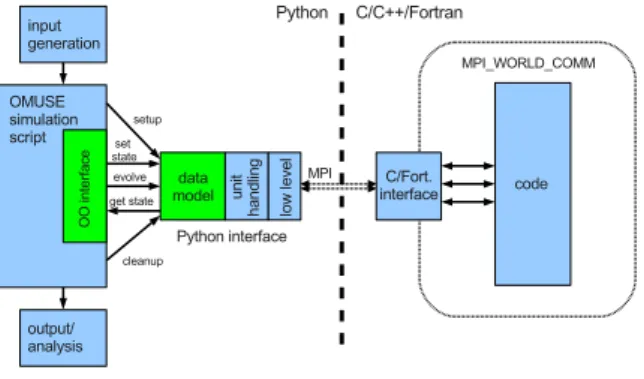
AnOMUSEapplication consists, roughly speaking, of auser script, aninterface layerand the community code base(Pelupessy et al., 2013), as illustrated in Fig. 1. The user script is constructed 85
by the user and defines a numerical experiment by specifying the initial data, the simulation codes to be used and the interactions between the codes. It may include analysis or plotting functions, in addition to writing simulation data to file. The setup and communication with a community code is handled by the framework in the interface layer, which consists of a communication interface with the community code as well as unit handling facilities and an object-oriented interface. The 90
interface layer also ensures the consistency of the interactions with the various simulation codes by maintaining a state model for each.
Figure 1. Design of theOMUSEframework. This schematic representation shows the design of the interface to a community code (“code”) and the way it is accessed from theOMUSEframework. The code has a thin
layer of interface functions in its native language (e.g. Fortran) which communicates through an MPI message channel with the Python host process. On the Python side, the user script (“OMUSEsimulation script”) makes
only generic calls to a high-level interface. This high-level interface calls the low-level interface functions, hiding details about units and the code implementation (the communication through the MPI channel does not interfere with the code’s own parallelization because the latter has its own MPI_WORLD_COMM context). Adapted from Pelupessy et al. (2013).
(1) qg=QG()
(2) qg=QG(debugger="gdb")
(3) pop=POP(number_of_workers=8)
(4) pop=POP(channel_type="distributed", hostname="Cartesius",
number_of_workers=600)
Figure 2.Examples of the instantiation of simulation codes withinOMUSE. (1) simple instantiation on a local
machine of theQG, (2) instantiation of a code inside a debugger, (3) local instantiation of an MPI-parallel code (POP), (4) instantiation ofPOPon a remote machine for a massively parallel high resolution run through the
distributedchannel (see section 2.2).
are, apart from the addition of oceanographic codes: improvements in grid support, amongst these 95
support for curvilinear grids and extensive framework support for grid remappings and grid gener-ation routines. In addition, a number of domain specific units and utility libraries and support for various file formats, such as NetCDF (Rew and Davis, 1990) output, have been added.
2.1 Remote function interface
The interface to a community code is provided by a set of functions, each communicating with the 100
interface object (Fig. 2), transparent to this. Python provides the possibility of linking Fortran or C/C++ codes directly, however we found that a remote protocol provides two important benefits. First, it provides for build-in parallelism. The choice for an intrinsically parallel interface is much 105
preferable over an approach where parallelism is added a-posteriori, because unless great care is taken in the design, features can creep in that preclude easy parallelization later on. Secondly, a lot of existing simulation codes are not written in a way that allows for multiple instances. They may, for example, use global variables or assume a single global state. This makes it unwieldy to instantiate multiple copies of the same code when linking directly. Using remote function interfaces means that 110
the codes run as separate executables, and thus this problem cannot occur (in addition this prevent collisions between incompatible libraries when the codes are built with different compilers).
Within the remote data communication channel, the MPI protocol can be replaced by a different method, two of which are currently available: a channel based on sockets and one based on eStep2 technology for distributed computing. At present, the sockets channel is mainly useful for cases 115
were a component process is to be run on one machine. As its name implies, it is based on standard TCP/IP sockets. The distributed channel is described in section 2.2 below. When using the MPI channel, different MPI implementations can be used (e.g.OpenMPIorMPICH), but not mixed.
The interface works as follows: when an instance of an imported simulation code is made, an MPI process is spawned as a separate process somewhere in the MPI cluster environment. This pro-120
cess consists of a simple event loop that waits for a message from the Python side. It will make the requested subroutine calls on the basis of the incoming message ID and any additional data that may follow the initial MPI message, and subsequently send the results back (Portegies Zwart et al., 2013). Since there is no direct memory access, the interfaces themselves must be carefully designed to ensure all necessary information for a given physical domain can be retrieved. Additionally, the 125
communication requirements between processes must not be too demanding. Where this is not the case (e.g. when a strong algorithmic coupling is necessary) a different approach may be more appro-priate.
Note that the interface design allows the parallelism of MPI parallel codes to be maintained even when the communication channel uses MPI (OMUSEcan be used to run massively parallel codes with 130
thousands of processes). This is guaranteed with the recursive parallelism mechanism in MPI-2. The spawned processes share a standard MPI_WORLD_COMM context, which ensures that an interface can be build around an existing MPI code with minimal adaptation (Fig. 1). Other parallelization paradigms, such as OpenMP, are also supported withinOMUSE. In practice, for the implementation of the interface for an MPI code, one has to reckon with similar issues as for the stand-alone MPI 135
application. The socket and distributed channels also accommodate MPI parallel processes. The choice between the different available channels depends on the computing resources needed for a
(1) q = 1. | units.Sv
dt= 1. | units.day
(2) (q*dt).as_quantity_in(units.m**3)
(3) (q*dt).value_in(units.km**3)
(4) def Reynolds_number(vel, length, visc):
return vel*length / visc
(5) R = Reynolds_number( 0.1 | units.cm/units.s, 1000. | units.km,
1.e-6 units.m**2/units.s)
Figure 3.An illustration of the use of theOMUSEunit algebra module, with (1) definition of a scalar quantity using the|operator, (2) conversion of a quantity to different units, (3) conversion of quantity to float, (4)+(5) definition of a function and its call using quantities.
given run. For runs distributed over remote machines the distributed channel may be required, while locally on a cluster the MPI channel often provides the most optimized communciation path.
2.2 Distributed computing 140
Current computing resources available to researchers are more diverse than simple workstations: clusters, clouds, grids, desktop grids, supercomputers and mobile devices complement stand-alone workstations, and in practice one may want to take advantage of this ecosystem.
To run in such a "Jungle computing environment" (Seinstra et al., 2011),OMUSEimplements a communication channel based on eStep technology (Drost et al., 2012). This channel starts a daemon 145
and connects with it, to communicate with remote workers. This daemon is aware of local and remote resources and the middleware (e.g. SSH) over which they communicate. The daemon uses the Xenon library to start the worker on a remote machine, executing the necessary authorization, queueing or scheduling automatically. BecauseOMUSEcontains large portions of C, C++, and Fortran, and requires a large number of libraries, it is not copied automatically, but it is assumed to be installed 150
on the remote machine. A binary-only release can be generated for resources, such as clouds, that employ virtualization. With these modifications,OMUSEis capable of starting remote workers on any computer the user has access to, without significant effort required from the user. From the user point of view, to use the distributed resources, anyOMUSEscript can be distributed by simply adding properties to each worker instantiation in the script, specifying the channel used, as well as the name 155
of the resource, and the number of nodes required for this worker (see Fig. 2).
2.3 Unit conversion
In order to simplify the handling of units, a unit algebra module is included inOMUSE(Fig. 3). This module wraps standard Python numeric types or Numpy arrays, such that the resulting quantities (i.e. a numeric value together with a unit) can transparently be used as numeric types (see the function 160
(1) grid=new_cartesian_grid((100,100))
(2) grid.ssh=0. units.m
(3) subgrid=grid[0:50,0:50]
(4) channel=QG.grid.new_channel_to( grid )
(5) channel.copy_attributes( ["psi"] )
(6) channel.transform( ["ssh"], lambda x:f0/g*x, ["psi"])
Figure 4.Example usage of the high-level grid data structure: (1) initialization of an empty Cartesian grid, (2) defining an attribute, here a scalar field of sea surface height (3) subgrid generation by indexing, (4) definition of an explicit channel from in-code storage to a grid in memory (5) update of grid attributes over the channel, (6) functional transform over a channel.
need extensive modification to work withOMUSEquantities (and in many cases work without any changes, if they are formulated in a dimensionally consistent way).
OMUSEenforcesthe use of units in the interfaces of the community codes. The specification of the unit dimensions of the interface functions is part of the interface specification (much in the same 165
way as the data types of the functions). Using the unit-aware interfaces, any data that is exchanged within modules will be automatically converted without additional user input, or - if the units are not commensurate - a code exception is generated. Keeping track of different systems of units and the various conversion factors when using different codes quickly becomes tedious. Enforcing the use of units therefore eliminates an important source of errors.
170
2.4 Data model
The interfaces to the code send low-level data types (e.g. an array of floats) over the remote function channel. While this is simple and closely matches the underlying C or Fortran interface, it needs considerable duplicated bookkeeping in the user script if used directly. Therefore, in order to sim-plify working with the codes, a data model is added to the interfaces based on the construction of 175
high-level objects that store the data (Fig. 4). Two base data stores are available: Particle sets and Grids (the main difference between these are that Particle sets can be extended dynamically and are unordered, while Grids are fixed when generated, ordered and can be multidimensional). These data stores can either reference memory in the main Python memory space (for sets defined independent of any code) or reference the data in the (possibly distributed) memory space of the community 180
code. Subsets can be defined on the sets without additional storage (see fig. 4, these subsets are im-plemented as views on the underlying local or remote data) and new sets can be constructed using simple operations.
2.4.1 Grid support
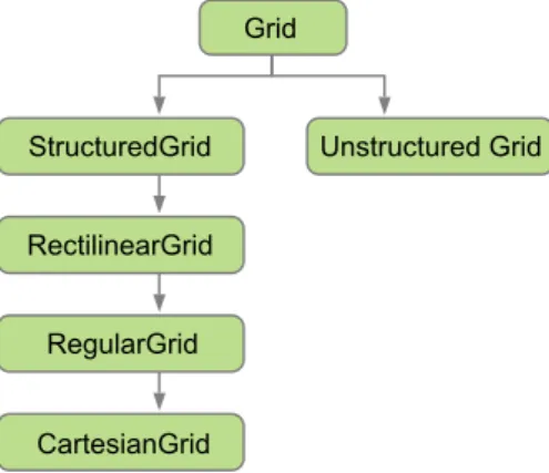
Compared toAMUSE,OMUSEexpands the support of grid data structures by introducing different 185
StructuredGrid Unstructured Grid Grid
RectilinearGrid
RegularGrid
CartesianGrid
Figure 5.Hierarchy of grid data types in OMUSE. Arrows denote inheritance of the corresponding classes in
OMUSE.
slicing, the creation of save points, and the creation of grid copies that include part or all of the grid attributes. The new grid types form a hierarchy (fig. 5), where each grid type has its own set of (derived) grid attributes (such as cell sizes) and utility functions (for basic operations, such as checking overlap or the extent of a grid). The grid types supported are: Cartesian (single, constant 190
cell size in each dimension), Regular (constant cell size per dimension), Rectilinear (cell boundaries specified per dimension), Structured (cells specified by a grid of corner points) and Unstructured (cell corners are specified for each cell individually).
2.4.2 Grid remappings
Grid remapping is a fundamental operation for coupled climate models, where heat and water fluxes 195
are periodically transferred between different component models, each using different grids inter-nally. In many cases, these remappings must be performed in an energy or mass conserving manner to maintain the global conservation conditions of the coupled climate system. As such,OMUSE in-terfaces withCDOfor their implementation of a second-order conservative remapping scheme (see section 3.2). However, different remapping backends can be used withinOMUSE.
200
OMUSEextendsAMUSEwith support for remapping quantities between different grids (AMUSE included support only for copying data between two equivalent grids).OMUSEallows the user to instantiate grid remapping objects. The remapper is initialized by setting the source and destination grid and can be used to remap a list of grid attributes from one grid to the other.
The use of such a remapping object is illustrated in Fig. 6, where as an example, the sea surface 205
(1) pop = POP(...)
(2) source = pop.elements
(3) adcirc = Adcirc(...)
(4) target = adcirc.elements
(5) remapper = conservative_spherical_remapper(source, target)
(6) remapper.forward_mapping(["ssh"])
Figure 6.Example usage of the high-level grid remapping functionality inOMUSE. In this example, the grid attributessh(for ‘sea surface height’) is remapped from the source grid to the target grid, both stored inside
the community codes, using a second-order conservative remapping scheme (the default). Unit conversions are performed automatically by the interface of the receiving community code.
needed, unit conversion of the values transferred between the models is automatically performed by the interface of the receiving code, as explained in section 2.3.
210
Support for remapping between unstructured grids, is limited in theCDOlibrary. Conservative interpolation of fields represented on unstructured mesh discretisations (Farrell et al., 2009) is being generalised in thelibsupermeshlibrary (libSupermesh, 2016) and could be utilised in the future.
2.5 State model
The internal work flows of different codes are in general not the same, even if they represent similar 215
physics. This can be due to the differences in the algorithms or simply because of design choices. For example, a change in one of the grid variables may necessitate a reinitialization of variables in one code, while in another code this may not be needed. It is easy to add the corresponding functions for such reinitialization to the interface. The problem with this is that it introduces differences between the interfaces, and is obviously error prone if controlled by the user. In order to manage this, the 220
interfaces inOMUSEcan be supplied with a representation of the work flow of a code. This is done in the form of a graph consisting of model states as the vertices and the transitions between them as the edges. Model states each have a set of allowable interface function calls. Such an interface call can trigger a transition between states (and for each transition there is a respective interface function). With thisstate modelOMUSEkeeps track of the state of a, changing the state when needed 225
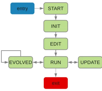
(and calling the corresponding interface methods). The state model will change state automatically if an operation is requested that is not allowed in the current state. If the request can not be fulfilled an error is returned. The state model is flexible: states can be added and removed as required. Most codes can be made to conform to a simple state model similar to the six state model shown in Fig. 7.
2.6 Object-oriented interfaces 230
Figure 7.Example of a state model inOMUSE. The diagram gives the states that a simulation code can be in. Transitions between these can be triggered by explicit calls to the corresponding function (e.g.
initialize_codefrom START to INIT) or implicitly (e.g. querying the grid state of a code may only be possible in the RUN state, and in this case the framework will call the necessary functions in order to get to the RUN state, guaranteeing a consistent state of the simulation code in the process). Adapted from Pelupessy et al. (2013).
different codes and the details of the code are hidden as much as possible. A lot of the bookkeeping (arrays / unit conversion) is absent in the high-level interface formulation. This makes the high-level 235
interface much easier to work with and less prone to errors: the user does not need to know what internal units the code is using, and does not need to remember the calling sequence nor the specific order of calls.
2.7 IO
Community codes that are included intoOMUSEwill usually contain subroutines to read in and write 240
simulation data. This functionality is preferably not used withinOMUSE. Instead, all simulation data is to be written and read from within theOMUSEscript (although in practice there can be reasons to retain some of the original functionality as part of the interface).OMUSEincludes a default output format based on HDF53that writes out all data pertaining to a data set, effectively standardizing the IO for all the codes included in the framework. In order to simplify import and export of data,OMUSE 245
contains a framework for generic I/O to and from different file formats. A number of common file
formats used in the oceanographic and climate modelling community are implemented (ADCIRC grid files, netCDF), as well as generic table format file readers.
2.8 Data analysis
After a simulation, the generated data needs to be analyzed. Python has good numerical and plotting 250
libraries available, such as Numpy and Matplotlib (Dubois et al., 1996; Hunter, 2007), and thus data analysis can be easily incorporated into theOMUSEworkflow. While the simulation codes are run-ning their internal state (as exposed through the interface) is accessible. This provides opportunities for efficient online data analysis, and also monitoring (or visualizing) the state of a running simula-tion. Based on the state of the model, the simulations can also be scripted beyond what is originally 255
implemented in the simulation code (examples of the latter are event-driven data output, or repeat simulation / resampling according to predefined conditions).
3 Component modules
In the present version,OMUSEcontains an initial set of ocean models, namelyQG,ADCIRC,POP andSWAN(ideally one would like te reach a ’Noah’s arc’ milestone, Portegies Zwart et al. (2009), 260
of having at least two independent application codes per domain). The implementation inOMUSEof the code interfaces is described in this section. The models cover different physics and / or a ranges of validity. and allow for are a number of different couplings between them. They also represent different levels of complexity in terms of code implementation, numerical schemes and a variety of discretizations (described below). In addition to the simulation codes,OMUSEalso contains support 265
codes, including for example theCDOpackage introduced above in section 2.4.2 which is used to implement remapping schemes between different grids.
3.1 Simulation codes
3.1.1 QG
OMUSEincludesQG, a code to calculate the dynamics of quasi-geostrophic ocean flow. The flow on 270
aβ−plane with Coriolis parameterf=f0+β0yis described by the barotropic stream functionψ
of the depth-integrated current velocityu= (u, v), with zonal velocityu=−∂ψ/∂yand meridional velocityv=∂ψ/∂x.QGsolves the governing barotropic vorticity equation (BVE) forψ(Pedlosky, 1996),
∂ ∂t∇
2ψ+J(ψ,∇2ψ) +β 0
∂ψ ∂x=
1 ρ0H
∂τy
∂x − ∂τx
∂y
−RH∇2ψ+AH∇4ψ, (1)
275
where the JacobianJ, here representing the advection of relative vorticity, is defined by
J(F, G) =∂F ∂x ∂G ∂y− ∂F ∂y ∂G
andτ= (τx, τy)represents the wind stress.QGcan also solve for the first baroclinic mode of a
mode expansion of the continuously stratified quasi-geostrophic vorticity equation (Flierl, 1978). The parametersρ0andHare the reference ocean density and reference ocean depth, respectively.
280
RHandAHare the bottom and lateral friction coefficients.QGsolves (1) on a rectangular domain
using a Cartesian grid. Boundary conditions consist of no-mass flux and/or no tangential stress (see for example Dijkstra and Katsman, 1997).
TheQGcode is written in Fortran 90 and uses the Poisson solver from thefishpack4or Intel MKL5libraries (depending on compiler). Although conceptually simple,QGprovides an instructive 285
case study for importing a code inOMUSE, with its relatively simple internal state and without the complications of coordinate transformations, and serves as a template for other ocean models in
OMUSE.
3.1.2 POP
The Parallel Ocean Program (POP) is a parallel global circulation model for ocean flows that solves 290
the three-dimensional primitive equations for a stratified fluid using the hydrostatic and Boussinesq approximations (Smith et al., 2010).POPis often used to calculate strongly eddying ocean circula-tion models. However, resolving eddies on a scale that captures the instabilities that lead to ocean eddies requires the use of a high-resolution grid. Such high-resolution runs are computationally ex-pensive, andPOPis also frequently used for simulations at lower resolutions, in this case the effect 295
of eddies is captured using sub-grid parameterizations (Gent and McWilliams, 1990).
ThePOPgrid is a structured 2D grid in the horizontal dimensions, usually in a dipolar or tripolar configuration.POPrequires that the grid dimensions are set at compile time. Therefore, we currently support two modes in whichPOPcan be used through theOMUSEinterface. The high-resolution mode assumes a grid size of3600×2400, corresponding to a 0.1◦resolution. The low-resolution 300
mode assumes grid dimensions of320×384horizontal grid points, corresponding to a 1.0◦resolution with tropical stretching. Vertically, the grid contains 40 or 42 non-equidistant layers, increasing in thickness from several meters near the surface to 250 meters just above the lower boundary at 6000 meters.
OMUSEinterfaces with a version ofPOP(based on version 2.1) that contains several extensions 305
(van Werkhoven et al., 2014)6. This implementation includes a flexible load-balancing scheme and optionally uses Graphics Processing Units (GPUs) to accelerate compute-intensive parts of the code. Considering the fact that it takes at least 1000 simulated years to reach a near statistical equilibrium state, it is common practice to restartPOPfrom a spun-up solution. The so-called ‘restart file’ and other settings can be set through theOMUSEPython interface after the code has been instantiated 310
and reached the ‘START’ state (see Fig. 7).
4www2.cisl.ucar.edu/
As with all codes inOMUSE, thePOPinterface employs a state machine that tracks the model state and ensures consistency by automatically calling the appropriate transition functions in the low-level interface. To be able to set many of the configuration options through the Python interface it was necessary to split several of the initialization routines in thePOPsource code. This was 315
required because these routines used to read their configuration from a namelist file and immediately proceeded to initialize the model using that configuration. WithinOMUSE, the model parameters are set through the interface as part of the Python script.
As such, the namelist file is only used to provide the code with default settings. After the settings have been read from the namelist, the model halts and waits for the settings that are specific to 320
the experiment to be passed through the interface. When the user has completed configuring the experiment, the state machine will automatically call a state transition function to complete the model initialization and advance the model to a state from which the user can interact with the model data or begin evolving the model.
ThePOPinterface provides two different ways to supply the model with forcings, such as wind 325
stress, surface heat flux, and surface freshwater flux. The first method is by setting the location of a file containing monthly averages of forcing data that will automatically be interpolated in time by the model. It is also possible to directly supply the model with forcing data through the interface, allowingPOPto be coupled with, for example, an atmospheric model. When forcing data is supplied through the interface,POPwill not use data from file for that type of forcing.
330
In theOMUSEexamples repository7, we have included an example Python script for setting up a POPrun in high-resolution mode in a cluster environment. The user script has to specify the location of the cluster head node and provide the requested number of nodes and cores and time required for the simulation. After that the user can instantiate the interface to create a running simulation and interact with the model.
335
3.1.3 ADCIRC
The Advanced 3D Circulation model (ADCIRC) solves the shallow water primitive equations on a triangular unstructured mesh in either two or three dimensions. Water surface elevationsζ, are obtained by solving the vertically-integrated continuity equation in the Generalized Wave Continuity Equation (GWCE) formulation (Leuttich and Westerink, 2004). The momentum equations are either 340
solved in vertically integrated form (2D mode), or in 3D (applying the Boussinesq and hydrostatic pressure approximations). In 3D,ADCIRCuses a generalized stretched vertical coordinate system (Leuttich and Westerink, 2004).
TheADCIRCmesh is represented in theOMUSEinterface as an unstructured grid of nodes and elements (which can be accessed as thenodesandelementsattributes of anADCIRCinstance), 345
representing the nodes and triangular elements of the grid. In the case ofADCIRCall prognostic
variables (with the exception of the wet-dry status of elements) are defined by a linearP1finite
el-ement Galerkin representation over the entire domain, described by coefficients associated to mesh node positions. For example, in the simplest 2D case these are the water level, its time derivative and the current velocities. The attributes of the elements are the nodes of each triangle, and its status 350
(indicating whether an element is dry or wet). In addition to this, the interface defines aforcings grid, which accepts the (possibly time-dependent) forcings. Depending on the parameters of the sim-ulation these can be for example wind stresses, atmospheric pressure, tidal potential, wave stresses etc. Boundaries are represented as sets of grids (one for each segment defined) with a reference to the nodes in the boundary segment, a type attribute (describing the type of boundary) and any ex-355
tra attributes necessary to specify the boundary condition (e.g. the water level for a boundary with prescribed elevations).
3.1.4 SWAN
In addition to the above models of hydrodynamical ocean circulation,OMUSEincludes an interface toSWAN(Simulating WAves Nearshore), a code to calculate the propagation of wind-driven surface 360
waves (Zijlema, 2010, and references therein).SWANuses a statistical description of the space and time varying wave properties, solving for the evolution of the action densityN(x, t;σ, θ), defined in terms of the wave energy density spectrumEasN=E/σ, whereNis a function of spacex, time t, relative radian frequencyσand directionθ. The evolution of the action density is governed by the action balance equation (e.g. Komen et al., 1994),
365
∂N
∂t +∇x·[(cg+U)N] + ∂(cσN)
∂σ + (∂cθN)
∂θ = Stot
σ , (3)
withcgthe wave group velocity,U the (depth averaged) current velocity,cσandcθthe
propaga-tion velocities in spectral and direcpropaga-tional space, respectively. The source/sink termStotrepresents
the physical processes which generate, dissipate or redistribute wave energy. Amongst them,SWAN includes generation of waves by wind, non-linear transfer of wave energy (including three- and four-370
wave interactions) and wave decay due to whitecapping, bottom friction and wave breaking (see SWAN, 2015, for more information).
SWANdiscretizes (3) on rectilinear, curvilinear (structured) or unstructured (triangular) grids in
one or two dimensions. TheOMUSEinterface toSWANsupports rectilinear and unstructured grids (curvi-linear grids can be added). The type of grid, as well as the type of grid for the forcings are 375
determined when the code is instantiated. Depending on the selected grid the interface defines a regular gridgridor an unstructured grid withnodesandelementsattributes. These have an attribute to access the action densityNof the grid. In addition to this, the bathymetry can be specified and a number of potentially time-varying forcing inputs, like water levels, water current velocities and wind velocities can be used (again a separate grid is used for the forcings).
To simplify the interface a few restrictions are placed on the forcings. For example, all the forcings in the interface use the same grid (whereasSWANsupports different grids for different forcings). This is not a limitation: withinOMUSE, any regridding (if necessary because the sources of the forcings use different grids) can be done on the framework level. If both calculation grid and input grid are unstructured, they are both assumed to use the same grid. In case of stationary calculations, the 385
interface still defines anevolve_model, but it simply calculates the stationary action density (for all input times). It can still make sense to evaluate this in a time dependent fashion, as the input forcings (and thus the equilibrium state) may change with time.
3.2 Support modules
In addition to the simulation codes, support modules written in different languages can be included 390
inOMUSE. Such a support module may, for example, provide functionality for coupling models. A support module can be interfaced with the same remote function interface as used for simulation codes. Currently, the only support module specific toOMUSEisCDOwhich is used for computing grid remapping weights and performing the remapping of quantities between different grids.
3.2.1 CDO 395
Climate Data Operators (CDO, 2015) is a command-line tool developed and maintained by the Max Planck Institute Hamburg containing over 400 operators that can process and manipulate climate data stored in self-describing file formats, such as netCDF.
AnOMUSEinterface toCDOwas created to be able to access the grid remapping functionality withinCDO. This library contains a reimplementation of the SCRIP package (Jones, 1999). The 400
remapping weights computed by SCRIP are used by other climate model couplers, such as the Model Coupling Toolkit (Jacob et al., 2005), and OASIS (Valcke, 2013). In particular, the second-order conservative remapping scheme implemented in SCRIP is used to compute remapping weights for conservative exchanges of (e.g. heat and water) fluxes at the ocean-atmosphere interface.
A number of minor code modifications were necessary to be able to access the functionality in 405
CDOas a library rather than as a command line tool. The low-level interface inOMUSEhas to ensure that the internal state ofCDOis consistent even though the code is not running as a command line tool. To do this, all grid information has to be propagated correctly to the different grid data storage structures used internally byCDO. In addition, the interface mimics some of the behavior ofCDOto produce the exact same results as when invoked from the command line. These include ignoring any 410
land masks in the source and target grids and increasing the number of search bins in the computation of remapping weights.
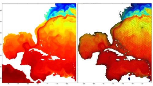
Figure 8.Result of a remapping performed by theCDOremapper using theOMUSEinterface. A sea surface
temperature field is remapped fromPOPusing a0.1◦tripole grid (on the left) to the elements of an unstructured grid (on the right).
and destination grids, as well as the remapping weights, (2) using netCDF files for storing source and destination grid information (as used byCDOand SCRIP) and (3) settingOMUSEgrid data types as source or destination grid. Modes (2) and (3) can be combined (if desired), and for these modes the remapping weights are computed automatically as the remapper initializes.
When using the default second-order conservative remapping scheme, the implementation ofCDO 420
also computes the gradients of the source field each time a quantity is being remapped. Note that the second-order conservative remapping scheme comes with limitations: the source grid has to be a structured grid because of the way SCRIP computes area integrals (for more information see the
CDOdocumentation).
In figure 8 we show the result of a remapping performed by theCDOremapper using theOMUSE 425
interface. A sea surface temperature field is remapped fromPOPusing a0.1◦tripole grid to an un-structured grid. The second-order conservative remapping scheme was used to compute the remap-ping weights based on the grid information presented by theOMUSEinterfaces of both simulations.
4 Code couplings
In addition to providing a unified interface to various types of codes,OMUSEhas the objective of 430
community codes can be combined into coupled models which have wider applicability than the original codes. The setup ofOMUSEallows for this in a transparent manner, such that the coupled 435
models have a similar interface as the individual models.
The types of coupling thatOMUSEcan be applied to is large, and range from simple input - out-put coupling to dynamic one-way coupling and to the development of two-way coupled solvers (see more examples Pelupessy et al. (2013)).OMUSEprovides the following features to facilitate the building of coupled models: simplified, uniform access to the code simulation state, unified inter-440
faces to the state of the simulation domain and its boundary conditions, and extensive automation of bookkeeping operations.
4.1 QG model coupling
Some care is needed in the design of the code interfaces to ensure that couplings are as simple as pos-sible. For example, the internal state of theQGsimulation consists of the stream functionψon two 445
time levels, these are represented as a grid object with attributespsi,dpsi_dtand positionsxand
y. It is more convenient to represent the two time levels as the (backward) time derivativedpsi_dt, because this representation is independent of the time step (which can be different between codes). The stream functionψ(and its derivative) can also be queried at any position using an interface func-tionget_psi_state_at_point. This function performs an (averaging) sampling and provides 450
a grid independent way to query and communicate the physical state. Another way to achieve this would be to perform a copy using a remapping channel as described in section 2.4.2.
In addition,QGhas two mechanisms to receive input from other codes: it calculates the evolu-tion of the stream funcevolu-tion using an input wind stress field. This wind stress field can be set by changing the wind stress attributestau_xandtau_yon theforcingsgrid. These can be copied 455
or remapped from another grid (read in from disk or generated dynamically by another code) or by defining a (time and or position depend) functional form (from an analytic wind model, for ex-ample). Other possible inputs are the boundary conditions:ψand∂ψ/∂ton the domain boundary. These consist of four grid objects (one for each cardinal direction) of sizeNo×2, whereNois the
number of grid points (in the corresponding dimension). Using these boundary grids it is possible 460
to implement two different strategies to vary the resolution over and/or the shape of the domain, namely grid nesting and domain decomposition.
4.1.1 Nested grid refinement
Depending on the parameters, equation (1) allows solutions with very narrow western boundary currents. Numerically this presents a challenge as the required resolution at this boundary may be 465
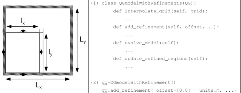
(1) class QGmodelWithRefinements(QG):
def interpolate_grid(self, grid):
...
def add_refinement(self, offset, ..):
...
def evolve_model(self):
...
def update_refined_regions(self):
...
(2) qg=QGmodelWithRefinement()
qg.add_refinement( offset=[0,0] | units.m, ...)
Figure 9.Schematic (left) and (abbreviated) definition of the refinedQGmodel class (right) with an example (2) of its instantiation.
a base grid with a refined region of higher resolution where the two grids are solved by separate instances of theQG.
470
Practically speaking, the following refinement strategy is followed (Fig. 9). Given a parent domain Lx×Lya refined sub domain is defined by its offset, extensionlx×lyand resolution dx. The low
resolution region consists of the whole domainLx×Ly(including the refined region). TheQGis used
to solve for the flow onLx×Ly. A second instance of theQGis used to solve the flow equation (1)
on the high resolution subdomainlx×lygiven appropriate boundary conditions. This high resolution
475
solution is then resampled and copied back (restriction operation) to correct the corresponding part of the domain on the low resolution grid.
If the boundary of the high resolution domain coincides with the boundaries of the parent domain (e.g. the east and south boundaries in Fig. 9) the boundary conditions are inherited from its parent. Otherwise, the boundary of the high resolution region lies in the interior ofLx×Ly, in this case
480
ψand∂ψ/∂tof the boundary can be obtained by interpolation of the low resolution grid. In our template implementation of this multigrid solver, we implement it as a derived interface inOMUSE (Fig. 9). It implements the same high-level interface (i.e. it has the same methods) as the baseQG, which allows these two to be used interchangeably. In particular, a refined region can itself have refinements.
485
4.1.2 Domain decomposition
This can be solved by iteration, but as the required step at each iteration (solving for∂ψ/∂tusing a Poisson solver) is quite expensive, this would be prohibitively inefficient. For this case, the problem can be accelerated by using accelerated vector extrapolation methods such as minimum polynomial extrapolation (MPE, Cabay and Jackson, 1976), i.e. we are solving for the fixed points of
xk+1=F(xk), (4)
495
wherexkis the vector consisting of the∂ψ
i/∂tvalues on the boundaries (of all mutually
neighbour-ing domains). In (4),Fis the operator determining the next vector in this sequence, with iteration indexk. This operator is provided by the instances of theQG, which calculates a new set of∂ψ/∂t values from previous set. The MPE method does not need explicit knowledge of the sequence gen-erator, and as such is especially well-suited for the problem here (this information in our case is 500
‘hidden’ in theQGcode). In practice the solution converges within a handful of iterations to satis-factory precision.
The evolve loop of a compoundQGconsisting of N domains then proceeds as follows: (1) update the internal boundaries of each domain N.ψ values are interpolated from neighbouring grids, a consistent set of∂ψ/∂tvalues are calculated using the MPE method. (2) all the domains are stepped 505
forward in time. An example of this will be shown in section 5.2 below.
Note that both preceding examples implement fairly close couplings. Nevertheless, theOMUSE framework can be used to implement these efficiently (both from the viewpoint of effort required to implement them as from a computational viewpoint. The most CPU intensive parts of the compu-tations (i.e. the solutions to the BVE (1)) are executed by the (optimized)QGsolver, while on the 510
framework level a limited amount of bookkeeping operations and data transfer is handled.
5 Applications
To demonstrate the capabilities ofOMUSEwe present a number of example applications. These illustrate the application of the unified interfaces ofOMUSEto calculate the same problem using different codes (section 5.1), the use ofOMUSEto implement intra-code domain decomposition 515
(section 5.2), a two-way coupling between codes with different physics (section 5.3), the embedding of a high resolution region in a low resolution domain using different codes (section 5.4) and the addition of data analysis to a running computation (section 5.5).
5.1 Critical transitions in a single-gyre ocean circulation model
The idealized classical model of a homogeneous mid-latitude wind-driven ocean (Sverdrup, 1947; 520
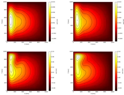
Figure 10.Comparison ofQGandADCIRCfor a simplified mid-latitude ocean configuration. Shown is the equilibrium SSH for a square domain basin of equal depth, driven by surface wind stress using the setup of Viebahn and Dijkstra (2014) (resulting in a single gyre solution) at two different Reynolds numbers:R= 1(top panels) andR= 10(bottom panels), whereR=U L/AHandU=τ0/(ρβ0LH)is a characteristic horizontal velocity. In each case, the left panel shows the solution obtained usingQG, and the right panel theADCIRC
solution is shown.
two completely different simulation codes to obtain equilibrium solutions and study the bifurcation diagram in a single-gyre setup (Viebahn and Dijkstra, 2014).
525
The first codeQGsolves the BVE (1), whileADCIRCsolves the primitive equations and does not impose the quasi-geostrophic approximation. In this sense this simple numerical experiment will illustrate a-posteriori the validity of the approximations made in deriving (1). We run theQG simulation for a 1000 km×1000 km basin with a resolution ofNo= 200×200with parameters
β0= 1.8616×10⁻¹¹(ms)−1RH= 0 s−1,AH= 1194 m2s−1, and a wind stress
530
τx=−τπ0cos(πy/L) ;τy= 0, (5)
whereτ0is determined by the adopted Reynolds numberR=τ0/(ρ0β0AHH)(ρ0= 1025 kg/m3
andH= 4000 m) ForADCIRC, a triangular grid matching this geometry is generated by subdividing the cells of a (No= 50×50) Cartesian grid into four triangles by adding a vertex to the center of
the cell. The parameters ofADCIRCare chosen to match the parameters inQG, and the same wind 535
0
5
10
15
20
25
30
35
40
45
Reynolds number
10
310
410
510
610
7ψ
[
m
2/s
]
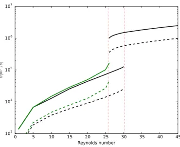
Figure 11.Part of the bifurcation diagram showing the upper and lower branches of steady and oscillatory solutions for a single gyre ocean model. Shown are the mean (dashed) and maximum (solid) value of the stream function forQG(black) andADCIRC(green) model runs, as a function of the Reynolds numberR. For
ADCIRCthe stream function is calculated asψ=gζ/f0, whereζis the free-surface height. The values shown represent time averaged values in case the system shows oscillatory behaviour. The flow undergoes a cyclic fold bifurcation nearR= 25as indicated by the vertical dashed lines (Viebahn and Dijkstra, 2014). TheADCIRC
solution becomes (numerically) unstable at this bifurcation.
In Figure 10 we compare the stable stationary solutions of the two codes (these are obtained by running until the maximum fractional changes in either stream functionψ(forQG) or sea surface elevationη(forADCIRC) between two successive diagnostic time intervals changes less than10−4). As can be seen, the two codes calculate solutions that agree well (although small differences can be 540
seen). Figure 11 shows the corresponding bifurcation diagram when varying the Reynolds number. The correspondence between the two codes is good for low Reynolds number, showing the same qualitative behaviour. At the bifurcation (aboveR≈25) we found that the solutions obtained by
ADCIRCbecome unstable to a basin-wide fast gravity wave mode, which is not represented in the
QGmodel. 545
5.2 QGon a composite domain
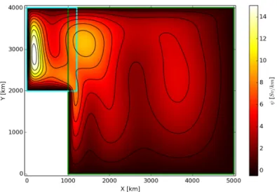
Figure 12.Stream functionψfor a non-rectangular domain run withQGon a composite domain. Plotted isψ
after 15 days of evolution with the compositeQGcode (section 4.1.2) on a domain consisting of two coupled subdomains, indicated by the cyan and green rectangles.
coupled solver presented in section 4.1.2 is employed for this. It uses separate instances ofQGto calculate the ocean flow (i.e. solutions to equation (1)) for a composite domain. In figure 12 the 550
solution is calculated on a domain with a western boundary that is stepped. The domain (shown in Figure 12) consists of a 4000×4000 km basin extended on the western side with a 1200×2000 km subdomain (the respective subdmains are indicated in the figure by the green and cyan rectangles). The solution is shown for a Reynolds numberR= 10, with similar single gyre forcing as (5) after 15 days of evolution (at this early stage one can distinguish the Rossby waves moving east to west 555
from the interior of the large basin, into the smaller domain).
Using such a composite domain it is possible to calculate the effects of topographic features on the dynamics of boundary currents, or change the resolution across the domain. Such idealized mod-elling on a simplified domain is often useful to reduce the real world topography to its essential fea-tures, e.g. Le Bars et al. (2012). The example above implements a tailored solver using the high-level 560
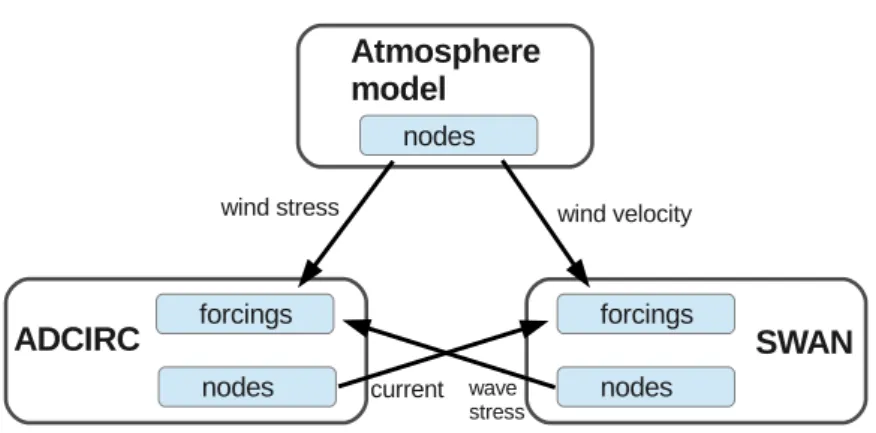
Figure 13.Schematic representation of theADCIRC-SWANcoupling.
(1) channel1=hurricane.grid.new_channel_to( swan.forcings )
(2) channel2=hurricane.grid.new_channel_to( adcirc.forcings )
(3) channel3=adcirc.nodes.new_channel_to( swan.forcings )
(4) channel4=swan.nodes.new_channel_to( adcirc.forcings )
(5) while time<tend:
(3) hurricane.evolve_model(time+dt/2)
(4) channel1.copy_attributes(["tau_x","tau_y"])
(5) channel2.copy_attributes(["vx","vy"])
(6) adcirc.evolve_model(time+dt/2)
(7) swan.evolve_model(time+dt/2)
(8) channel3.copy_attributes(["current_vx","current_vy"])
(9) channel4.copy_attributes(["wave_tau_x","wave_tau_y"])
Figure 14.Definition of communication channels and evolve step corresponding to figure 13.
5.3 Implementation of a coupled SWAN-ADCIRC model
The propagation of wind-driven surface waves is sensitive to water levels and current velocities. The properties of the underlying circulation will affect the evolution of the wind-driven wave field and the location of wave-breaking zones. On the other hand, wind-driven wave transport can generate radiation stress gradients that can in turn drive circulation set-up and currents. Currents can also be 570
affected by changes in the vertical momentum mixing and bottom friction stresses generated by the wind-driven wave field. Thus, in many coastal applications, such as the calculation of storm surges, waves and circulation processes should be mutually coupled.
Here we will demonstrate the implementation of such a coupling within theOMUSEframework, applying it to a coupling of theADCIRCcirculation model and theSWANwave propagation model. A 575
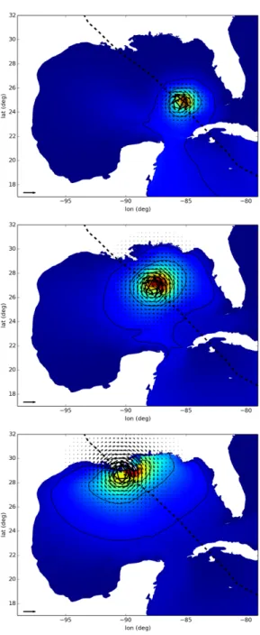
(some-Figure 15.Significant wave heights for hurricane Gustav (2008), calculated using a coupledADCIRC-SWAN
Figure 16.Schematic representation of thePOP-ADCIRCone way coupling for an embedded domain. The labelled arrows indicate the use of remapping channels. "remap" stands for a conservative remapping between the structuredPOPgrid and the unstructuredADCIRCgrid, while "interp." indicates that the variables are interpolated.
what simplified)OMUSEcode corresponding to this model coupling. Note that in this coupling both
SWANandADCIRCuse the same unstructured (triangular) grid. The communication between the 580
codes (as shown in Fig. 14) is handled bychannels, whereby the framework handles the copying (and unit conversion) of data.
As an example we apply the coupled code to calculate the wave height and storm surge of hurri-cane Gustav (2008)8in the Gulf of Mexico. The hurricane is modelled using an analytic prescription (Holland, 1980) from data of a hurricane storm track (positions, central pressures, maximum wind-585
speed, storm radius) read in from file. Implementation of this analytic model is in the form of a Python class mimicking a full simulation code.ADCIRCis run in 2D barotropic mode with meteo-rological forcing from the hurricane model andSWANprovides the wave stresses. There is no forcing on the open ocean boundaries. For the discretization of the action density,SWANuses 36 bins in the directional space and 32 bins in frequency (from 0.05 to 1 Hz). The standard set of third generation 590
wave parameters, including the effects of wave breaking, bottom friction and 3-wave interaction is used. The time step (dt) between updates of the coupled quantities is 600 seconds.
In figure 15 we show the resulting wave heights calculated by the model during the development of hurricane Gustav at three different times. The results of theOMUSEcoupling are similar to the re-sults of the integrated coupling implementation (Dietrich et al., 2011, and above mentioned website). 595
Technically the coupling as inOMUSEdiffers from the implementation by Dietrich et al. (2011), as the latter directly copies data in the unified memory space of a single binary (an for that reason is more efficient). However, both implement the same coupled processes and the approach taken by
OMUSEdoes not depend on the particular aspects of the selected codes - exactly the same script
(1) forcings_channel=pop_forcings_grid.new_remapping_channel_to(
adcirc.forcings, conservative_spherical_remapper)
(2) boundary_channel=pop_grid.grid.new_remapping_channel_to(
adcirc.elevation_boundary, interpolating_remapper)
(3) while time<tend:
(4) pop.evolve_model(time+dt/2)
(5) forcings_channel.copy_attributes(["tau_x","tau_y"])
(5) boundary_channel.copy_attributes(["ssh"])
(6) adcirc.evolve_model(time+dt)
(7) pop.evolve_model(time+dt)
(8) time+=dt
Figure 17.Definition and use of remapping channels for thePOP-ADCIRCembedding of figure 16.
Figure 18.Sea surface heights and velocities of aADCIRCrun embedded in a global circulationPOPmodel. Top panels show the sea surface height (SSH) of a region covering the Western North Atlantic Ocean, Caribbean Sea and Gulf of Mexico. The upper left panel shows the high resolutionADCIRCSSH field (superimposed on thePOPfield) and the upper right panel the low resolutionPOPfield. The black square indicated in the top
right panel is shown in more detail in the lower panels where the SSH with velocities superimposed are shown (in the case ofADCIRCthe barotropic velocities are shown, forPOPthe are the surface velocities). The dashed
5.4 Embedded regional model
A recurring problem for regional or coastal modelling is the application of realistic boundary condi-tions from the open ocean, even more so when one is interested in the effect of large scale or global processes on the regional level. One approach to obtain realistic boundary conditions at the required scale is the nesting of a high resolution and small scale model in a lower resolution but larger scale 605
model (e.g. Debreu et al., 2012; Djath et al., 2014).
Here we illustrate the implementation of (one-way) nesting inOMUSEby embedding a regional high resolution barotropicADCIRCmodel of the Caribbean and North American Atlantic coast into aPOPglobal circulation model (see fig. 16). In this case, sincePOPuses a curvilinear structured grid andADCIRCan unstructured triangular mesh, it is necessary to perform a remapping when 610
transporting variables from one code to the other (these functionalremappingchannels are indicated in figure 16 by the labelled arrows).
For the actual implementation of the coupling inOMUSE, the difference between using a remap-ping channel and a normal (data copying) channel (such as the ones used in section 5.3) is small: the only difference with a normal channel is that upon initialization the actual remapping method to 615
be used needs to be specified for a new remapping channel. The usage of the remapping channel to prescribe the data flow in the coupled model (figure 17) uses the same semantics.
In order to calculate the dynamics of the nested regional model,ADCIRCin 2D barotropic mode needs an input wind stress field and the specification of either the sea surface level or normal fluxes on the boundary. In addition to this, the model can be initialized from remapped flow variables 620
(barotropic velocities and sea surface heights). Note that a fully consistent coupling between the two codes is not possible since they solve for a different set of variables (2D barotropic vs 3D baroclinic). For the (conceptual) example here, a coupling was made on the sea surface elevation, and the bathymetry of theADCIRCgrid was limited to 500m depth (so the barotropic basin represented in
ADCIRCcan only be compared with the upper 500m layer ofPOP). The time step for the coupling 625
(updates of the boundary surface elevations) is taken to be equal to thePOPinternal time step of approximately 30 minutes. The remappings are performed at each time step for the wind stresses and for the sea surface heights.
Figure 18 shows the sea surface heights and velocities on the original low resolutionPOPgrid and the embedded higher resolutionADCIRCgrid after 30 days of adjustment (after this theADCIRC 630
solution follows the (slow) variations ofPOP). A fully consistent coupling is possible when using
ADCIRCin baroclinic mode. In this case, the coupling proceeds (with a larger number of coupling
variables involved) along similar lines.
8The data for this example comes from:
5.5 On-the-fly data analysis
In addition to consuming massive amounts of CPU time, current large scale simulations are capable 635
of generating enormous amounts of data. Usually, it is possible to store only a very limited subset of this data, this limits the data analysis that can be performed. One solution to this has been to do (part of) the analysis on the fly. Online data analysis offers several opportunities, including the fact that special actions can be taken when interesting events occur. Such special actions may include inspecting the model internal data at resolutions, both spatial and temporal, that are not available or 640
feasible with offline data analysis. While running simulations throughOMUSE, the simulation state is accessible, and this allows for data analysis while a simulation is running.
As a proof-of-concept application we add an online ocean eddy tracker on top of thePOPmodel. The interest in ocean eddies comes from the fact that eddies transport considerable energy and mass and as such influence the dynamics of large-scale ocean circulation and the climate (e.g. 645
Viebahn and Eden, 2010; Griffies et al., 2015). To understand eddy properties and variability, several mesoscale eddy tracking algorithms have been proposed in recent years. We have adapted a sea sur-face height-based eddy tracking code that is implemented in Python, calledpy-eddy-tracker (Mason et al., 2014). The code uses high-pass filtered sea level anomaly (SLA) fields. On the filtered fields, contours are computed at 1 cm intervals for levels between -100 cm to 100 cm. These contours 650
are then searched to locate eddies based on their shape, area, and amplitude.py-eddy-tracker tracks eddies across successive sea level anomaly (SLA) fields using a search ellipse, bounded by the local (long baroclinic) Rossby wave speed.
We have generalized the code in order to use different data sources, including output that is ob-tained directly from numerical models. To this end, we have modified thepy-eddy-trackerto 655
be able to handle grids that contain gaps, as land-only blocks are not part of the simulation in POP. We useBasemap9to compute a landmask for the given grid and apply it to the SLA field. Finally, we have created a simple, but easy to use, interface to thepy-eddy-trackerthat understands the grid data structures and units used inOMUSE.
Figure 19 shows the code required to build an online eddy tracking program withOMUSE. The 660
interfaceEddyTrackeris given theOMUSEgrid datatype used byPOPand automatically per-forms unit conversions and extracts the information that it needs (i.e. the sea surface height and the coordinates of the grid points).
Figure 20 shows the output of the online eddy tracking program that uses sea surface height data directly from a runningPOPsimulation. In this image, we can clearly see the large anticyclonic 665
eddies that result from the retroflection of the Agulhas Current, as well as many smaller eddies being tracked over time by the online eddy tracking algorithm. The data generated by the online eddy tracker can, for example, be used to compare the statistics of the simulated eddies to the analysis made usingpy-eddy-tracker(or other tools) of altimetry data.
from omuse.ext.eddy_tracker.interface import EddyTracker from omuse.community.pop.interface import POP
p=POP( ... ) #start POP as you would do normally
dt_analysis = 7 | units.day
tracker = EddyTracker(grid=p.nodes, domain=’Regional’, lonmin=0. | units.deg, lonmax=50. | units.deg,
latmin=-45. | units.deg, latmax=-20. | units.deg, dt_analysis)
tnow = p.model_time
stop_time = p.model_time + (1 | units.yr)
while (tnow < stop_time):
p.evolve_model(tnow + dt_analysis)
tracker.find_eddies( ssh=p.nodes.ssh, rtime=p.model_time ) tnow = p.model_time
tracker.stop(tend) p.stop()
Figure 19.This example demonstrates how to build an application that analyzes data from a running simulation usingOMUSE. This code implements an online eddy tracking program that tracks the eddies based on sea surface
height every seven days for one year ofPOPsimulation.
6 Summary and Discussion 670
We have presented the Oceanographic Multipurpose Software Environment (OMUSE) which pro-vides a homogeneous interface to existing or newly-developed ocean models. As illustrated by the results in the previous section, the use cases forOMUSErange from running simple numerical ex-periments with single codes (e.g. section 5.1), to combining simulation codes and data analysis tools (section 5.5) and setting up fairly complicated and strongly coupled solvers (section 5.2) to solve 675
problems that are intrinsically multi-scale (section 5.4) and/or require different physics (section 5.3). UsingOMUSE, simulations can be easily scripted and on-the-fly data-analysis can be added.
The implementation of the different use cases is facilitated by several aspects of theOMUSE de-sign.OMUSEdefines standardized interfaces and data structures for different codes. The data struc-tures and the state model as well as the communication model used inOMUSEare flexible and allow 680
a wide variety of codes, written in different languages, to be integrated withOMUSE.OMUSEalso works well with established methods to generate initial conditions and analyze the resulting data.
OMUSEshares some of the goals of a number of other coupling frameworks that have been
devel-oped in the earth system modelling community (e.g. Hill et al., 2004; Buis et al., 2006; Gregersen et al., 2007; Jacob et al., 2005; Larson, 2005; Peckham et al., 2013; Valcke, 2013). The closest equivalent 685
is the Community Surface Dynamics Modeling System (CSDMS; Peckham et al., 2013).CSDMSand
Figure 20.Output of the online eddy tracking application using data from a runningPOPsimulation, showing a
region around the southern tip of Africa. The green lines show the contours between areas of different sea level anomaly values. Red indicates areas of elevated sea level, and is used to detect anticyclonic eddies. Similarly, blue indicates a lower sea level, and is used to identify cyclonic eddies. The red or blue lines indicate the track that an eddy has travelled since it was first detected.
inter-operability since the interface components of theCSDMScould be easily adopted for anOMUSE interface (and possibly vice versa). TheCSDMSBMI (basic model interface) and CMI (component 690
model interface) are roughly equivalent to theOMUSElow and high-level interfaces, respectively The main differences betweenOMUSEandCSDMSare that the former presents Python as the main user interface for programming an application, while for theCSDMSthere are various choices, in-cluding a GUI frontend. In addition,OMUSEsimplifies the interaction with the community codes using high-level object-oriented data structures andOMUSEhas a more extensive and flexible state 695
model.
It is important to ensure the accuracy, reliability and reproducibility of a integrated framework like
OMUSE. We employ a number of strategies to ensure this is the case. The framework itself is tested daily and upon the commit of changes using more than 2000 component tests that cover approxi-mately 80% of the framework code and range from basic tests of the interfaces to the simulation 700
-SWANcoupling) the results of a coupled solver implemented withinOMUSEcan be compared with a reference coupling implementation (Dietrich et al., 2011, e.g.). In any case, to ensure the correctness 705
of a new application inOMUSEone should conduct the usual tests to ensure the validity and verify the results.
An important concern of a coupling framework such asOMUSEis performance. While the initial driver for the development ofOMUSEis to simplify the setup and development of coupled simu-lations, the architecture ofOMUSEis designed with a high degree of parallelism. The internal data 710
structures are efficient. Also the individual simulation codes are often highly optimized. So the per-formance of anOMUSEapplication is rarely a concern, but this is strongly problem dependent. In practice, the overhead imposed by the framework is often measured to be rather small (less than a few percent), but it is not difficult to formulate problems where the strength of the coupling is intrin-sically so strong that very frequent communication between the component solvers is necessary. 715
In this respect a limitation of the current design ofOMUSEis the fact that the communication between solvers is handled by the master script. This imposes a bottleneck for the performance of the communication between e.g. two parallel codes. While in the current setup there are some mitigating techniques that can be applied (asynchronous communication or grouping and spawning the communication-intensive subprocesses), ultimately we would need to implement adistributed 720
communication channel that would direct the data flow from the sending to the receiving process directly. Note that such distributed communication channels would not change the semantics of the use of a channel between data structures.
Code availability
The main framework and community modules are production ready.OMUSEis foreseen to grow over 725
time with new codes and capabilities.OMUSEis freely downloadable10and comes with a testing framework and basic examples. Furthermore, it can easily be adapted for private use (the licence is GPL3).
We distribute the simulation codes that are interfaced byOMUSEtogether with the framework, if the authors distribute their code with an open source licence, otherwise these codes must be down-730
loaded separately. New codes or extensions, as well as bug fixes may be submitted to the repository.
OMUSEencourages the practice of distributing simulation codes by reporting automatically, upon
conclusion of anOMUSEscript, which community codes were used during the run and suggesting references for inclusion in any publications.
Extending OMUSE 735
The effort required to import or interface a code withinOMUSEvaries with the code complexity, and depending on whether a similar code already exists within the framework (in this respect the codes