5224.pdf

(1)

The Influence of Parceling on the Implied

Factor Structure of Multidimensional Item

Response Data

Brooke E. Magnus

A thesis submitted to the faculty of the University of North Carolina at Chapel Hill in partial fulfillment of the requirements for the degree of Master of Arts in the Department of Psychology

Chapel Hill 2013

Approved by:

David M. Thissen, PhD

Patrick J. Curran, PhD

(2)

Abstract

Brooke E. Magnus: The Influence of Parceling on the Implied Factor Structure of Multidimensional Item Response Data

(Under the direction of David M. Thissen, PhD)

(3)

Acknowledgement

(4)

List of Tables

Page

1 Allocation of Items to Parcels in Study #1 . . . 19

2 Simulation Design for Primary Goal #1 . . . 20

3 Simulation Design for Primary Goal #2 . . . 20

4 Bifactor Model # 1: Estimated Factor Loadings of Parceled Continuous Data . . . 21

5 Bifactor Model # 1: Correlation of Factor Score vs. Theta from Generating Model . . . 22

10 Bifactor Model # 1: Estimated Factor Loadings of Parceled Dichotomous Data . . . 25

11 Bifactor Model # 1: Correlation of Factor Scores vs. Theta from Generating Model . . . 25

12 Average Model Fit Statistics for Continuous Data . . . 26

13 Average Model Fit Statistics for Dichotomous Data . . . 26

14 Item-Level Factor Loadings . . . 32

15 HPI Factor Correlations . . . 34

16 Correlations of HPI Parcels . . . 34

17 Estimated Factor Loadings of Parceled HPI Data . . . 34

19 Bifactor Model # 2: Correlation of Factor Scores vs. Theta from Generating Model . . . 45

(6)

List of Figures

Page

1 3-Factor Model with Simple Structure . . . 5

2 Cattell’s Radial Parceling. Reprinted from “Radial parceling vs. item factoring in defining personality structure in questionnaires: Theory and experimental checks,” by R. B. Cattell, 1974,Australian Journal of Psychology,26, pp. 107. . . 7

3 Bifactor Model . . . 15

4 Bifactor Model with 28 Items . . . 18

5 Follow-Up Study Design . . . 28

6 Estimated Factor Loadings from CFA vs. Primary Factor Loadings from Generating Model . 29 7 Correlations between Estimated Factor Scores and True Values of the Generating Model. Note the diﬀerent vertical scales used for the primary and secondary factors. . . 31

8 HPI Factor Structure . . . 33

9 Inverse Schmid-Leiman Transformation: Bifactor Model to Oblique Structure . . . 41

10 Bifactor Model #1 . . . 42

11 Bifactor Model #2 . . . 43

(7)

Introduction

What is Parceling? A Literature Review

1. Item-Level Data in Factor Analysis

Several assumptions underlie factor analysis. The use of item-level data in place of essentially con-tinuous indicators can pose many threats to the tenability of these assumptions if the item-level analyses are not carried out with proper technique.

One assumption of traditional linear-normal factor analysis is that the relationships between the observed variables and latent variable(s) are linear. When the observed variables are responses to the Likert-type or dichotomous items that are common in psychology and education, this relationship cannot be linear, violating this important assumption of traditional factor analysis. Another potential problem with using item-level data is that individual items usually have relatively low reliability and communality (Little, Cunningham, Shahar, & Widaman, 2002). Lower reliabilities and communalities are likely to lead to poorer fitting factor analysis models, and without good fit, the model has little practical utility. The distribution of individual item responses also deviates from normality if it is not continuous. An indicator’s departure from normality can introduce bias when estimating factor loadings and residual variances.

(8)

are estimated using traditional linear, normal, factor analysis methods are relatively unstable, requiring a great number of iterations before convergence (Kline, 2005).

2. What are parcels?

One technique for handling the problems that arise in the use of item-level data in factor analysis is known as parceling (Cattell, 1956). Parceling involves grouping items or scales together, either by aver-aging or summing two or more indicators, reducing the number of indicators that go into the estimation of the model parameters. Parcels can group items according to various criteria, such as item discrimina-tion or content, or the grouping can be random. It is important to note that diﬀerent researchers may define item parcels diﬀerently. For example, Kishton and Widaman (1994) specify that item parcels are psychometrically unidimensional, whereas Cattell (1956) makes no reference to the unidimensionality of items in the formation of parcels. This may seem like a small distinction, but it can have implications for the research being conducted, as will be seen throughout the remainder of this thesis.

2.1 Parcels in Educational Research

Broadly speaking, two major areas of research have made use of item parcels: educational research and psychological research. In educational research, tests are primarily used for the purpose of scoring. As previously mentioned, the binary items so common in educational testing create a non-linear relationship between the item and factor. This violates the assumption of linearity in traditional factor analytic methods, causing the model to be misspecified when fit using the traditional common factor model (Bandalos & Finney, 2001). Parceling has been proposed to circumvent this problem, as summing binary items lengthens the response scale, resulting in approximately continuous and nearly normally distributed parcel scores.

(9)

research is usually performed only on data where the dimensionality has alreadsy been examined. This is not universally true of research using parcels, as will be seen in the next section.

2.2 Parcels in Psychological Research

A second area of research where parceling is commonly used is attitude and personality measurement within psychology (Bandalos & Finney, 2001). Personality research often has the aim of identifying the factor structure of items or scales; scoring is not typically the goal. The rationale for parceling provided by psychological researchers includes better model fit, minimized influence of sampling error, reduction of idiosyncrasies in the responses, improvement of indicator reliability, better item to subject ratio, satisfaction of the assumption of multivariate normality, and the avoidance of estimation problems common in item-level analysis (Bandalos & Finney, 2001; Sass & Smith, 2006). There are a number of issues with these justifications for using item parcels. First, the better fit often obtained through the use of parcels is attributable to minimizing the sources of lack of fit. One of these sources of lack of fit can be sampling error (MacCallum, Widaman, Zhang, & Hong, 1999). If this is the case, parceling can be seen as innocuous, if not advantageous; however, better fit is often obtained by masking another source of variance: multidimensionality in the data (Little et al., 2002). In empirical data analysis it is impossible to determine which source of variance is being masked by parceling. Further, model fit should not be the goal of factor analysis. Rather, the goal should be to explain as accurately as possible how latent constructs influence observable indicators (Bandalos & Finney, 2001).

Another reason psychological researchers oﬀer for using item parcels is to reduce the idiosyncrasies of the data (Marsh, Hau, Balla, & Grayson, 1998). While it is true that parceling tends to lessen the eﬀects of these idiosyncrasies, if item responses are so idiosyncratic that they have a large amount of unique variance, perhaps these items are not actually measuring the construct they purportedly measure. This calls into question the construct validity of the items, which suggests that the items should not be used in the first place. Improved reliability of the indicators is another commonly cited reason for using parcels (Yuan, Bentler, & Kano, 1997); however, this is true by necessity, and the extent to which this is valid depends on the reliability of the original items. Finally, some researchers claim that they cannot use factor analysis and other latent variable models because they have too few subjects and too many items in the study, and that parceling will improve the item to subject ratio, making latent variable modeling a feasible technique. While this reason has some merit, the item to subject ratio may not actually be as important if the communalities of the items are high (MacCallum et al., 1999).

(10)

groups, it is imperative to ensure that the same measurement properties hold across models. The first step in testing for measurement invariance is typically to test whether all groups exhibit the same factor structure. To test for this, the same model is fit to all groups, and fit statistics are considered to determine the degree to which the model fits the data across all groups. Therefore, attaining acceptable model fit for every group is necessary to argue that measurement invariance holds. For all of the reasons previously mentioned, item-level analyses can yield poorly fitting models. Therefore, parceling is an attractive method of improving model fit for researchers wishing to show measurement invariance. The first potential problem with using parcels as indicators in tests of measurement invariance is that model fit can become inflated as an artifact of using parcels, not because the model is correct. Meade and Kroustalis (2006) tested this notion by assessing the influence of parceling on measurement invariance tests of factor loadings, intercepts, and uniqueness terms. They simulated item-level responses for one group, and then introduced diﬀerential item functioning into some of the items for the second group. They conducted measurement invariance tests on both the item-level responses and parcels of responses, where clusters of four item responses were combined to form a parcel. To test for measurement invariance, a series of likelihood-ratio tests was conducted sequentially, depending on the type of measurement invariance that was being considered. Their results indicated, most importantly, that the use of parcels can mask a lack of measurement invariance. Researchers would falsely conclude that all items have the same measurement properties across groups when in fact they do not. For these reasons, the authors strongly suggest that only item-level data, not parcels, be used in measurement invariance research. Diﬀerent configurations of item-level factor loadings can result in the same configuration of parcel factor loadings. This is a concept that will recur when reviewing other simulation studies.

3. Parceling Methods

The literature describes several diﬀerent types of item parceling. While there are many names for these methods, they typically reduce to either isolated uniqueness or distributed uniqueness strategies, terms coined by Hall, Snell, and Foust (1999). To facilitate an understanding of the diﬀerence between these two methods, consider a three-factor model, in which three items load on each factor and exhibit simple structure, as seen in Figure 1. The sections that follow will refer to this model.

3.1 Isolated Uniqueness

(11)

Factor 1

Factor 2

Factor 3

Item 1

Item 2

Item 3

Item 4

Item 5

Item 6

Item 7

Item 8

Item 9 Figure 1. 3-Factor Model with Simple Structure

of a single dimension. In the three-factor example, each parcel corresponds to one of the three factors. If following the model in Figure 1, Parcel 1 consists of Items 1, 2, and 3, Parcel 2 consists of Items 4, 5, and 6, and Parcel 3 consists of Items 7, 8, and 9.

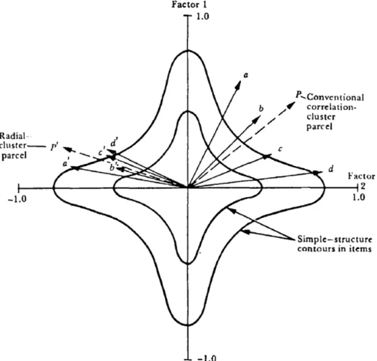
Radial Parceling Radial parceling is the type of parceling advocated by Cattell (Cattell, 1956, 1974; Cattell & Burdsal, 1975). This method of parceling involves a preliminary item factor analysis before any parcels are formed, “to give the first rough indications of the dimensions and parcel factoring” (Cattell, 1974, p. 103). The method behind radial parceling is to cluster items based on the cosines describing their relations in a factor space, not their correlations. To demonstrate the eﬀects of radial parceling, Cattell considered four items: a,b,c, andd. For itemsa andd, their correlation is given by

rad=hahdcosad (1)

whereh2

(12)

While the correlation between the two items in both sets is the same, their cosines are diﬀerent, with the cosine of the angle between itemsb andc being much larger than the cosine of the angle between items a and d. The resulting parcel of items a andd forms vector_P~_{, which points in a direction away from}

any true hyperplane (i.e., Factor 1 or Factor 2). Cattell’s goal was to develop a method ensuring that only items located as close together on a hyperplane as itemsa0_,_b0_, _c0_{, and} _d0 _{should ever be combined}

into the same parcel (see quadrant IV of Figure 2, where the vector _P~0 _{associated with the resulting}

parcel is in the direction of a true hyperplane). This is accomplished by combining items based on the matrix of cosines rather than the matrix of correlations. The other important distinction Cattell made with his radial parceling technique is that all parcels should comprise the same number of items. Many subsequent articles have addressed the question of number of items per parcel, (e.g., Bandalos & Finney, 2001; Bandalos, 2002), but to the author’s knowledge, none have advised that each parcel must have the same number of items. This is an issue that seems to have disappeared from the literature since it was originally proposed by Cattell.

While Cattell did not refer to his method of parceling asisolated uniquenessas subsequent researchers have done, it is likely that this is the type of parceling to which he was referring in his papers. His radial parceling strategy involves forming unidimensional parcels, comprising only those items that are being influenced by the same underlying factor. This is an important qualification that is often neglected by researchers citing Cattell to justify the use of parcels. Bandalos and Finney (2001) surveyed the parceling literature and found that only 32% of the research employing item parcels referred to the dimensionality of their data. This is one of the main issues that this thesis addresses.

3.2 Distributed Uniqueness

(13)

Figure 2. Cattell’s Radial Parceling. Reprinted from “Radial parceling vs. item factoring in defin-ing personality structure in questionnaires: Theory and experimental checks,” by R. B. Cattell, 1974, Australian Journal of Psychology,26, pp. 107.

4. Existing Studies

Many empirical and simulation studies have been conducted that attempt to examine the influence of parceling on both unidimensional and multidimensional data. Some of them focus only on the measure-ment model (i.e., confirmatory factor analysis), while others extend to full structural equation models. The next section will discuss several of these studies, including their methodologies and results, and attempt to identify questions that remain unanswered.

4.1 Unidimensional Data

(14)

item-level data, using parcels formed from the item-level data, and using the scale as a single indicator but accounting for measurement error by fixing the factor loading to reflect the index of reliability and the error loading to reflect the error variance. They used both simulated and empirical data and found that as long as the assumption of unidimensionality is satisfied, the estimates of the disattenuated structural coeﬃcients between latent variables in a structural equation model did not change, whether using item-level data, parcels, or the reliability-corrected single indicator in building the measurement model. They concluded that the structural coeﬃcient estimates do not change when items are parceled, because the measurement error of the indicators is reorganized rather than changed; however, this does not mean that the parameter estimates of the measurement model remain the same. They found that the factor loadings became larger when parcels were used as opposed to items, because parcels are better indicators of latent constructs than individual items. Sass and Smith (2006) concluded that the choice of whether to use parcels or item-level data should depend on the interest of the researcher. If the primary research question relates more to the validity of the measurement model, then it is more appropriate to use item-level data. Parceling can change the results and interpretation of the factor loadings. However, if the research question is more about the relationship between latent variables and the measurement model is not of great interest, then parceling is an appropriate technique, assuming unidimensionality. Yuan et al. (1997) argue that if the items are truly unidimensional – that is, when the measured variables are influenced by only one latent variable – parceling will not alter the original factor structure. In this context, the method of parceling is irrelevant; all methods should produce the same factor structure, whether parceling is conducted randomly or systematically.

4.2 Multidimensional Data

(15)

isolated uniqueness methods would lead the researcher to correctly reject the misspecified model. Hall et al. (1999) concluded by suggesting that the isolated uniqueness strategy be used when the item set is relatively unidimensional (the secondary construct is much weaker than the primary construct), but that the distributed uniqueness strategy may be preferable in cases where the data are truly multidi-mensional. They also suggested that future research examine the eﬀects of parceling when there are multiple secondary constructs influencing items.

Bandalos (2002) also examined the eﬀects of parceling multidimensional data. To test whether the parceling method can obscure the true factor structure, she fit a misspecified two-factor model to data generated from a three-factor model, where the third factor was a secondary factor onto which some items cross-loaded. She employed the isolated and distributed uniqueness strategies. Results revealed that the use of parcels can suggest deceptively good fit, even when the model is misspecified, as it was in her study. The distributed uniqueness strategy was worse in terms of leading to falsely retaining the misspecified model; more models were judged to fit well when in fact they did not. Bandalos concluded that item parceling should be used when items have a known factor structure, and that multidimensional parceling should be discouraged.

Rogers and Schmitt (2004) expanded on the research of Hall et al. (1999) and Bandalos (2002) by introducing a more complicated factor structure to the measurement model. They included two or four secondary influences, as opposed to the single secondary influence that was present in Bandalos (2002) and Hall et al. (1999). The isolated vs. distributed uniqueness strategies no longer yielded substantially different results in terms of parameter bias and model fit. The authors surmised that this was due to the presence of multiple secondary influences; therefore, the data exhibited much more multidimensionality than in the other studies. Consequently, isolating the uniqueness was much more difficult, and the isolated uniqueness strategy effectively behaved the same as the distributed uniqueness strategy.

(16)

substantively meaningful factors emerged. These items were then parceled in such a way that either all the items comprising a sub-factor were put into the same parcel (isolated), or they were balanced evenly across parcels (distributed). When comparing the results from the two diﬀerent parceling methods, they found that both were eﬀective in that good model fit for three factors was attained, but that only the distributed uniqueness strategy led to acceptable parameter estimates. The use of the isolated uniqueness strategy resulted in inadmissible parameter estimates. While their results might suggest that distributed uniqueness parceling is preferable, the authors made no such claim, urging other researchers to use caution in interpreting the results of a parcel factor analysis.

While there are many papers that examine the effects of parceling on the measurement model (i.e., factor loadings), fewer studies have looked at the effects of parceling on the structural coefficients in a full structural equation model. Coffman and MacCallum (2005) compared the structural coefficients when four different measurement methods were used: homogeneous parcels, heterogeneous parcels, total (aggregated) path analysis models, and path analysis models where reliability estimates were used to correct for measurement errors. When comparing these methods using simulated data, they found that homogeneous parcels produced the least biased estimates of the structural coefficients as well as the best overall model fit; heterogeneous parcels produced poorer fit and did not recover the population parameters as well as the homogeneous parcels, but they were still better than the relability corrected and total score path analysis methods. In the analysis of empirical data, homogeneous parcels produced the largest point estimates of the structural coefficients and correlations between the factors; however, the overall model fit was better when the heterogeneous parcels were used. Homogeneous parcels pro-duced unacceptable fit. Coffman and MacCallum (2005) argued that the worse fit exhibited under the homogeneous parceling method was due to less common varianace. When items that load on the same factor are placed into a single parcel, parcels are less similar to each other than if each parcel is formed to be a balanced representation of all factors. This results in greater unique variance, less common variance, and thus, poorer fit. Coffman and MacCallum (2005) concluded their study by recommending that, when given a choice between total path analysis based on summed scores as measured variables and a latent variable model that makes use of parcels, applied researchers use parcels as indicators of latent variables. They did not make any recommendations in terms of specific parceling methods.

5. What are researchers actually doing when they parcel?

(17)

Researchers have begun to address this question, mostly through simulation (e.g., Hall et al., 1999; Bandalos, 2002; Coﬀman & MacCallum, 2005), but since Cattell’s original papers of the 1950s, no one has considered the eﬀects of parceling from an analytic perspective. To understand why Cattell advocated the use of parcels, it is important to understand his mathematical rationale. His claims, along with the algebra he used to support them, follow.

5.1 Cattell’s Claims

Cattell first proposed item parceling in 1956 and published several subsequent papers on the topic (e.g., Cattell, 1973, 1974; Cattell & Burdsal, 1975). After the publication of his seminal paper in 1956, some researchers reacted with skepticism, claiming that the factor analysis of the parceled data is likely to lead one to draw diﬀerent conclusions than the factor analysis of the item-level data. Cattell (1974) insisted that the number of factors emerging from the parcels is same as the number of factors emerging from the item-level data, and substantiated his claim with an algebraic derivation. For a set ofnitems being influenced bykcommon factors,

aij =bj1T1i+bj2T2i+...+bjkTki+bjTji (2) where aij corresponds to person i’s score on item j, bjk represents the loading of item j on common factork, Tkirepresents personi’s factor score on common factor k, bj represents itemj’s loading on a unique factor, and Tji represents person i’s factor score on item j’s unique factor. Now consider two items,handj,

aih=bh1T1i+bh2T2i+...+bhkTki+bjThi (3)

aij =bj1T1i+bj2T2i+...+bjkTki+bjTji (4) in a domain wherekfactors account for the variability in these two items. Itemshandj have diﬀerent

loadings on factors 1 throughk, with the possibility of any or none being zero. Cattell showed that if

hand j are combined into a parcelpto form parcel score (a1h+a1j), the variance contributed to the parcel score (a1h+a1j) by factor T1 can be expressed as

2

(a1h+a1j)=b 2

h1+b2j1+ 2bh1bj1 (5)

(18)

2

(ah+aj)= k

X

x=1

(b2hx+b2jx+ 2bhxbjx) +b2h+b2j (6) Now, the loading of parcelpcontaining itemshandj on factork can be expressed as

bp=

b2h1+b2j1+ 2bh1bj1 2

(ah+aj)

(7)

This is for orthogonal factors, although the same result is found when the factors are permitted to correlate. Cattell remarked that because bp has the product term 2bh1bj1 in the numerator, which is

due to the summing of itemshandj to form the parcel, the loading on the common factor will increase

more quickly as items are added to the parcel than the loading on the specific factor:

b2

h1+b2j1 2 (ah+aj)

(8)

He used this logic to argue that “parcels with any degree of homogeneity (similarity of sign of loadings) will express and define the common factor space to a higher degree than will single items” (Cattell, 1974, p. 105).

Cattell’s proof can be summarized by stating that the parcel will have the same common factor dimensionality as the items that comprise it, except in cases where a) there is a common factor that exists only in items hand j and in no other items, in which case loading b will become specific, and

b) items h and j have loadings of the same magnitude but opposite directions. He concluded that

parcel and item factoring yield the same rotation and meaning, but that parceling oﬀers the advantage of more clearly defined common factors. It should be noted, however, that to support his claims, Cattell advocated only the use of radial parceling, which corresponds to the isolated uniqueness strategy previously discussed.

5.2 The Problem with Cattell’s Derivation

(19)

ignores the fact that these loadings came from an item factor analysis, which in itself has the problem of indeterminacy. Or worse, these same factors may or may not be detected in the factor analysis of the parcel scores. He based his derivation on the assumption that factor scores can be treated as observable variables. This assumption is not necessarily true, making his claims about the dimensionality of the factor structure also not necessarily true. For this reason, a further examination of the eﬀects of parceling on the model-implied factor structure is warranted.

6. An Algebraic Examination of Parceling

A review of the literature indicates that nearly all the studies done on item parceling have been simulations examining the eﬀects of parceling multidimensional data; however, analytics can show, to some extent, how the formation of parcels alters the factor structure of the data. Consider forming parcels using a transformation matrix T of dimension p_⇥n, where p is the number of parcels to be

created and n is the number of items. The T matrix comprises0s and 1s as its elements and selects

items into parcels, resulting in a simple sum of item scores that form a parcel score. Whether one is using the isolated or distributed uniqueness parceling strategy determines the placement of the0s and1s

in theT matrix (Sterba & MacCallum, 2010). For example, if a researcher wishes to form three 3-item

parcels from nine items using the isolated uniqueness strategy, it can be expressed as:

2 6 6 6 6 4

xp1

xp2 xp3

3 7 7 7 7 5= 2 6 6 6 6 4

1 1 1 0 0 0 0 0 0 0 0 0 1 1 1 0 0 0 0 0 0 0 0 0 1 1 1

3 7 7 7 7 5 2 6 6 6 6 6 6 6 6 6 6 6 6 6 6 6 6 6 6 6 6 6 6 6 6 4 x1 x2 x3 x4 x5 x6 x7 x8 x9 3 7 7 7 7 7 7 7 7 7 7 7 7 7 7 7 7 7 7 7 7 7 7 7 7 5 = 2 6 6 6 6 4

x1+x2+x3 x4+x5+x6 x7+x8+x9

3 7 7 7 7 5 (9)

(20)

2 6 6 6 6 4

xp1

xp2

xp3

3 7 7 7 7 5= 2 6 6 6 6 4

1 0 0 1 0 0 1 0 0 0 1 0 0 1 0 0 1 0 0 0 1 0 0 1 0 0 1

3 7 7 7 7 5 2 6 6 6 6 6 6 6 6 6 6 6 6 6 6 6 6 6 6 6 6 6 6 6 6 4 x1 x2 x3 x4 x5 x6 x7 x8 x9 3 7 7 7 7 7 7 7 7 7 7 7 7 7 7 7 7 7 7 7 7 7 7 7 7 5 = 2 6 6 6 6 4

x1+x4+x7 x2+x5+x8 x3+x6+x9

3 7 7 7 7 5 (10)

From these matrices, it is easily seen that theT matrix changes as a function of the type of parceling

one wishes to use. The column vector of parcel scores can then be expressed as xp p⇥1where

xp p⇥1

= T

p⇥n⇥nx⇥1 (11)

The covariance matrix of the parcel scores can be expressed as:

E(xpxTp) =E(T xixTiTT) =T⌃iTT (12)

whereT⌃iTT is the covariance matrix of the items, pre- and post-multipled by the transformation matrix

T. Applying the common factor model, the covariance matrix of the parcels,⌃xp, can be rewritten as

⌃xp=T(⇤i i⇤

T

i +⇥ i)T

T ₌_T_⇤

i i⇤TiTT +T⇥ iT

T ₍₁₃₎

To the author’s knowledge, Sterba and MacCallum (2010) were the first and only researchers to consider parceling from this algebraic perspective, although they did so in the context of simulation. Using this derivation, it is possible to factor analyze the model-implied parcel covariance matrix to compare the resulting factor loadings with the true factor structure.

6.1 An Example

(21)

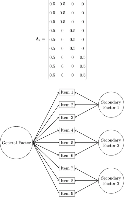
⇤i= 2 6 6 6 6 6 6 6 6 6 6 6 6 6 6 6 6 6 6 6 6 6 6 6 6 4

0.5 0.5 0 0 0.5 0.5 0 0 0.5 0.5 0 0 0.5 0 0.5 0 0.5 0 0.5 0 0.5 0 0.5 0 0.5 0 0 0.5 0.5 0 0 0.5 0.5 0 0 0.5

3 7 7 7 7 7 7 7 7 7 7 7 7 7 7 7 7 7 7 7 7 7 7 7 7 5 (14) General Factor Item 1 Item 2 Item 3 Item 4 Item 5 Item 6 Item 7 Item 8 Item 9 Secondary Factor 1 Secondary Factor 2 Secondary Factor 3

Figure 3. Bifactor Model

(22)

RIU =

2 6 6 6 6 4

1.000 0.375 0.375 0.375 1.000 0.375 0.375 0.375 1.000

3 7 7 7 7

5 (15)

Under the distributed uniqueness parceling method, the resulting correlation matrix is

RDU =

2 6 6 6 6 4

1.000 0.667 0.667 0.667 1.000 0.667 0.667 0.667 1.000

3 7 7 7 7

5 (16)

It is clear from the correlation matrices for both the isolated and distributed uniqueness strategies that a one-factor model is implied – all of the oﬀ-diagonal elements are the same. The associated factor loadings are 0.612 under isolated uniqueness and 0.785 under distributed uniqueness. It appears that a single latent factor is influencing the three parcel indicators. The true model could be considered either a bifactor model with one general factor and three orthogonal secondary factors, or a three-factor model with oblique simple structure (see Appendix A for this transformation); however, under no interpretation would this be considered a one-factor model as the parceling would lead one to conclude. This algebraic derivation demonstrates that parceling multidimensional data using either the isolated or distributed uniqueness techniques can lead one to incorrectly conclude that a single factor explains all the variance in the data.

(23)

Present Study: Method

1. Primary Goals

1.1 How does parceling change the estimand?

The primary goal of this project is to use analytic and computational approaches to show what happens when two types of data are parceled: continuous and categorical. Specifically, it is of interest whether the original parameter is truly being estimated, or if it is some other estimand that is estimated. From the examples of parceling demonstrated in the Introduction of this thesis, it is clear that in some cases parceling does in fact change the parameter being estimated. The questions that remain are 1) what are these cases, and 2) how does this new estimand relate to the original factor(s)? Answering these questions is the primary goal of this thesis.

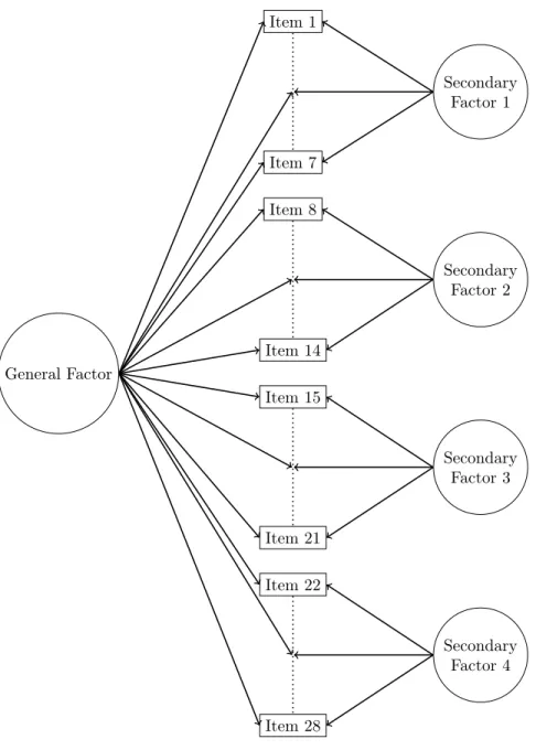
Continuous Data The algebraic derivation in the previous section illustrates the preliminary steps in answering the question of what happens when one parcels continuous data. Figure 4 depicts the structure of the bifactor models that were considered as part of these analyses. Transformation matrices were used to select the items into parcels according to either the isolated or distributed uniqueness parceling methods. Then, the item correlation matrix was pre- and post-multiplied by the transformation matrix that was used to parcel the items. A one-factor model was fit to the new correlation matrix, and the factor loading estimates were compared to selected factor loadings from the pre-parceled item-level factor analysis – specifically, the loadings on the general factor. Appendix B contains path diagrams of the bifactor models that were included in this analysis.

(24)

General Factor

Item 1

Item 7

Item 8

Item 14

Item 15

Item 21

Item 22

Item 28

Secondary Factor 1

Secondary Factor 2

Secondary Factor 3

Secondary Factor 4

Figure 4. Bifactor Model with 28 Items

(25)

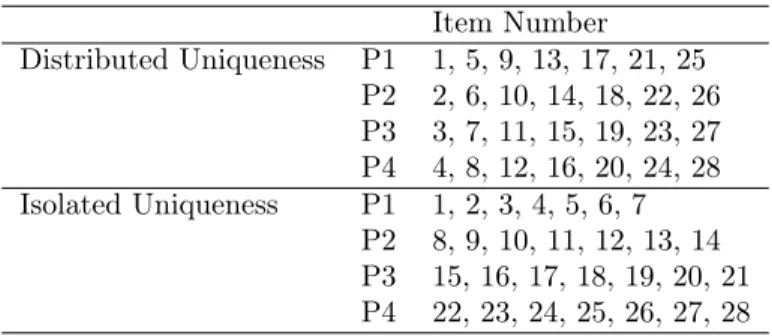
Table 1. Allocation of Items to Parcels in Study #1 Item Number

Distributed Uniqueness P1 1, 5, 9, 13, 17, 21, 25 P2 2, 6, 10, 14, 18, 22, 26 P3 3, 7, 11, 15, 19, 23, 27 P4 4, 8, 12, 16, 20, 24, 28 Isolated Uniqueness P1 1, 2, 3, 4, 5, 6, 7

P2 8, 9, 10, 11, 12, 13, 14 P3 15, 16, 17, 18, 19, 20, 21 P4 22, 23, 24, 25, 26, 27, 28

These item numbers correspond to those in Figure 4.

parceling strategy and then correlated with the general and secondary theta values from the generating model.

Categorical Data When data that are assumed to be on an underlying normal continuum are placed into discrete categories, there is a loss of information. As a result, when the Pearson product moment correlation between two dichotomous or Likert-type items is computed, attenuation occurs: the Pearson correlation is always an underestimate of the true correlation that exists between the underlying con-tinuous variables. Consequently, item covariances cannot be derived from the common factor model as in the continuous case; however, the population-level item covariances can still be computed. For two dichotomous items,X1 andX2 ₂[0,1]:

Var(X1) = E(X12) (EX1)2= E(X1) (EX1)2, (17)

Cov(X1, X2) = EX1X2 EX1EX2, (18)

which reduces to the computation of the first two moments of item responses. Within a two-parameter logistic item response theory (2PL IRT) framework,

EX1=P(X1= 1) =

Z

T1(1|✓) (✓)d✓ (19)

EX1X2=P(X1= 1, X2= 1) =

Z

T1(1_|✓)T2(1_|✓) (✓)d✓, (20)

whereTj(xj|✓)is the multidimensional trace line function

T(Xj= 1|✓) = 1

(26)

computed, transformation matrices can be applied to select items into parcels, as done in the continuous case. After fitting a one-factor confirmatory factor analysis (CFA) to the parcel covariance matrix, factor loading estimates are considered the limit of those that would be obtained by applying this procedure to sample item covariance matrices. Using this method, it was possible to study analytically the patterns in estimated factor loadings across diﬀerent models and parceling methods for categorical data as well as continuous data. To examine how sampling variability aﬀects the estimates, a simulation analogous to that for the continuous case was also performed. The design of the simulation can be found in Table 2.

Table 2. Simulation Design for Primary Goal #1

Data Type Bifactor Model Sample Size Parceling Method Continuous Model #1, Model #2, Model #3 100, 500 Isolated, Distributed Dichotomous Model #1, Model #2, Model #3 100, 500 Isolated, Distributed Design: Data Type x Bifactor Model x Sample Size x Parceling Method

1.2 When do goodness of fit statistics deceive?

Parceling can lead to improvement in model fit at the expense of masking model misspecification (e.g., Hall et al., 1999; Bandalos, 2002). A second primary goal of this thesis was to identify the cases in which model fit improves despite a misspecified model. To identify these cases, the 2 _{and RMSEA}

statistics were examined after fitting the (misspecified) one-factor model to the parceled data. The question of interest was the proportion of times the researcher would falsely accept the one-factor model as being the data-generating model, and whether this proportion diﬀered between the two parceling methods.

Table 3. Simulation Design for Primary Goal #2 Data Type Sample Size Parceling Method Continuous 100, 500 Isolated, Distributed Dichotomous 100, 500 Isolated, Distributed Design: Data Type x Sample Size x Parceling Method

2. Secondary Goal

2.1 Empirical Data Analysis

(27)

data were parceled according to the isolated and distributed uniqueness parceling methods and then fit with a one-factor CFA.

Present Study: Results

1. Continuous Data

1.1 Bifactor Model # 1

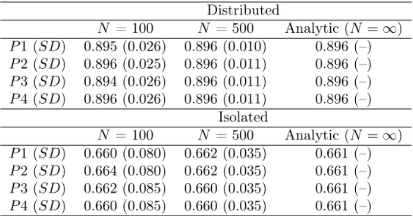
The estimated factor loadings of the parceled data for Bifactor Model # 1 can be found in Table 4. These estimates are obtained after fitting a one-factor CFA to four parcels of seven items each, according to either the isolated or distributed uniqueness parceling strategies. For each parceling method, results of the simulations based on sample sizes of 100 and 500 are presented, as well as the analytic solution derived using covariance algebra. As can be seen from these results, the factor loading estimates for the distributed uniqueness parceling method are consistently higher than those for the isolated uniqueness method. Additionally, as sample size increases, the estimated factor loadings more closely approximate those derived analytically. Increase in sample size also results in decreased variability in the estimated loadings across the four parcels.

Table 4. Bifactor Model # 1: Estimated Factor Loadings of Parceled Continuous Data Distributed

N = 100 N = 500 Analytic (N =₁)

P1 (SD) 0.895 (0.026) 0.896 (0.010) 0.896 (–)

P2 (SD) 0.896 (0.025) 0.896 (0.011) 0.896 (–)

P3 (SD) 0.894 (0.026) 0.896 (0.011) 0.896 (–)

P4 (SD) 0.896 (0.026) 0.896 (0.011) 0.896 (–)

Isolated

N = 100 N = 500 Analytic (N =1)

P1 (SD) 0.660 (0.080) 0.662 (0.035) 0.661 (–) P2 (SD) 0.664 (0.080) 0.662 (0.035) 0.661 (–) P3 (SD) 0.662 (0.085) 0.660 (0.035) 0.661 (–) P4 (SD) 0.660 (0.085) 0.660 (0.035) 0.661 (–)

(28)

distributed uniqueness method are likely slightly smaller than those that would have been estimated had each parcel been exactly equally representative of the secondary factors.

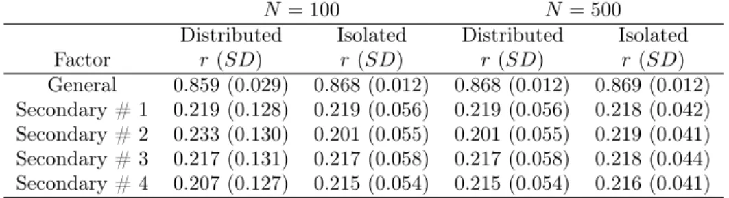
To examine how well the factor scores from the parceled data recover the general factor from the generating model, estimated factor scores were computed under each parceling strategy; these factor scores were then correlated with each of the theta values from the generating model. Factor scores were calculated using the traditional linear regression method. Table 5 displays these correlations. Across both sample sizes and parceling strategies, factor scores are most highly correlated with the general factor. These correlations range from 0.859 to 0.869. Correlations with the secondary factors are substantially lower, ranging from 0.207 to 0.233. There do not appear to be diﬀerences between the two parceling methods in the degree to which the parcel-based model recovers the general factor from the generating model.

Table 5. Bifactor Model # 1: Correlation of Factor Score vs. Theta from Generating Model

N = 100 N = 500

Distributed Isolated Distributed Isolated Factor r(SD) r(SD) r(SD) r(SD)

General 0.859 (0.029) 0.868 (0.012) 0.868 (0.012) 0.869 (0.012) Secondary # 1 0.219 (0.128) 0.219 (0.056) 0.219 (0.056) 0.218 (0.042) Secondary # 2 0.233 (0.130) 0.201 (0.055) 0.201 (0.055) 0.219 (0.041) Secondary # 3 0.217 (0.131) 0.217 (0.058) 0.217 (0.058) 0.218 (0.044) Secondary # 4 0.207 (0.127) 0.215 (0.054) 0.215 (0.054) 0.216 (0.041)

The second bifactor model weakened the proportionality constraints imposed in the first model. Instead of all primary and secondary loadings remaining constant at 0.5, secondary loadings varied across secondary factors; factor loadings for items within a secondary factor were equal. All loadings on the general factor were 0.5. Table 6 shows the estimated factor loadings from the CFA based on the parceled data.

Compared to Bifactor Model # 1, there is more variability in the estimated parcel loadings, especially in the isolated uniqueness condition. Estimated factor loadings approach the values from the analytic derivation as sample size increases. As true of Bifactor Model # 1, estimated loadings for this model are always higher for the distributed uniqueness parceling method than the isolated uniqueness parceling method.

(29)

N = 100 N = 500 Analytic (N =1)

P1 (SD) 0.897 (0.025) 0.897 (0.012) 0.897 (–) P2 (SD) 0.888 (0.026) 0.890 (0.013) 0.890 (–) P3 (SD) 0.897 (0.024) 0.897 (0.011) 0.897 (–) P4 (SD) 0.903 (0.024) 0.904 (0.010) 0.904 (–)

Isolated

N = 100 N = 500 Analytic (N =1)

P1 (SD) 0.710 (0.076) 0.707 (0.033) 0.711 (–) P2 (SD) 0.666 (0.082) 0.662 (0.035) 0.661 (–) P3 (SD) 0.606 (0.089) 0.612 (0.039) 0.613 (–) P4 (SD) 0.656 (0.084) 0.663 (0.036) 0.661 (–)

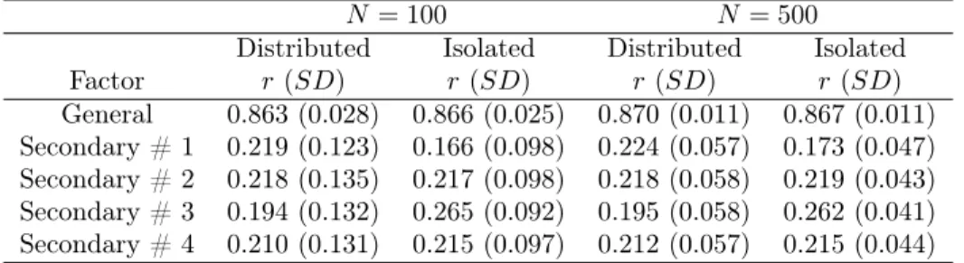
Bifactor Model # 1: factors scores are much more highly correlated with the general factor than any of the secondary factors, and this is true across parceling method and sample size.

N = 100 N = 500

Distributed Isolated Distributed Isolated Factor r(SD) r(SD) r(SD) r(SD)

General 0.863 (0.028) 0.866 (0.025) 0.870 (0.011) 0.867 (0.011) Secondary # 1 0.219 (0.123) 0.166 (0.098) 0.224 (0.057) 0.173 (0.047) Secondary # 2 0.218 (0.135) 0.217 (0.098) 0.218 (0.058) 0.219 (0.043) Secondary # 3 0.194 (0.132) 0.265 (0.092) 0.195 (0.058) 0.262 (0.041) Secondary # 4 0.210 (0.131) 0.215 (0.097) 0.212 (0.057) 0.215 (0.044)

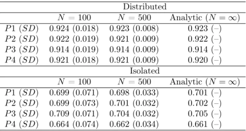
The third bifactor model futher weakened the proportionality constraints of the previous two models. Unlike the first two models in which the loadings on the general factor were the same across all items, this model had general factor loadings that varied depending on the secondary factor that was influencing the set of items. There were proportionality constraints in place such that within a secondary factor, the higher the loading on the general factor, the higher the loading on the secondary factor. Table 8 contains the estimated factor loadings for the four parcels for both parceling strategies.

As with the other two bifactor models, distributed uniqueness parceling produces the largest factor loadings. For both sample sizes, these loadings tend to be very close to the analytic values; increasing the sample size does not change the estimate, although the standard deviations are smaller. Under isolated uniqueness, sample size does aﬀect the estimate. The larger sample size produces estimates that are closer to the values derived analytically.

(30)

N = 100 N = 500 Analytic (N =1)

P1 (SD) 0.924 (0.018) 0.923 (0.008) 0.923 (–) P2 (SD) 0.922 (0.019) 0.921 (0.009) 0.922 (–) P3 (SD) 0.914 (0.019) 0.914 (0.009) 0.914 (–) P4 (SD) 0.921 (0.018) 0.921 (0.009) 0.920 (–)

Isolated

N = 100 N = 500 Analytic (N =1)

P1 (SD) 0.699 (0.071) 0.698 (0.033) 0.701 (–) P2 (SD) 0.699 (0.073) 0.701 (0.032) 0.702 (–) P3 (SD) 0.709 (0.071) 0.704 (0.032) 0.705 (–) P4 (SD) 0.664 (0.074) 0.662 (0.034) 0.661 (–)

N = 100 N = 500

Distributed Isolated Distributed Isolated Factor r(SD) r(SD) r(SD) r(SD) General 0.881 (0.024) 0.886 (0.022) 0.886 (0.010) 0.886 (0.010) Secondary # 1 0.199 (0.127) 0.189 (0.098) 0.206 (0.055) 0.196 (0.041) Secondary # 2 0.211 (0.122) 0.224 (0.091) 0.221 (0.057) 0.232 (0.043) Secondary # 3 0.229 (0.124) 0.207 (0.095) 0.213 (0.055) 0.201 (0.043) Secondary # 4 0.189 (0.125) 0.202 (0.100) 0.189 (0.055) 0.202 (0.043)

the generating model. Consistent with the previous two bifactor models, estimated factor scores are much more highly correlated with the general factor from the generating model than the secondary factors, for both isolated and distributed parceling methods.

2. Dichotomous Data

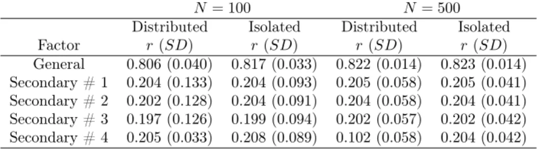
A similar pattern of results was found with the dichotomous data, which were generated from a 2PL IRT model. Table 10 contains the estimated factor loadings for the first bifactor model. As with the continuous data, the distributed uniqueness parceling strategy results in greater factor loadings than isolated uniqueness. Note that the estimated loadings are smaller for the dichotomous data than for their continuous counterpart.

(31)

Table 10. Bifactor Model # 1: Estimated Factor Loadings of Parceled Dichotomous Data Distributed

N = 100 N = 500 Analytic (N =1)

P1 (SD) 0.779 (0.052) 0.778 (0.023) 0.777 (–) P2 (SD) 0.779 (0.053) 0.779 (0.022) 0.777 (–) P3 (SD) 0.777 (0.055) 0.777 (0.023) 0.777 (–) P4 (SD) 0.776 (0.053) 0.779 (0.023) 0.777 (–)

Isolated

N = 100 N = 500 Analytic (N =1)

P1 (SD) 0.596 (0.105) 0.593 (0.043) 0.591 (–) P2 (SD) 0.591 (0.101) 0.592 (0.045) 0.591 (–) P3 (SD) 0.591 (0.100) 0.591 (0.042) 0.591 (–) P4 (SD) 0.589 (0.100) 0.589 (0.043) 0.591 (–)

Table 11. Bifactor Model # 1: Correlation of Factor Scores vs. Theta from Generating Model

N = 100 N = 500

Distributed Isolated Distributed Isolated Factor r(SD) r(SD) r(SD) r(SD) General 0.806 (0.040) 0.817 (0.033) 0.822 (0.014) 0.823 (0.014) Secondary # 1 0.204 (0.133) 0.204 (0.093) 0.205 (0.058) 0.205 (0.041) Secondary # 2 0.202 (0.128) 0.204 (0.091) 0.204 (0.058) 0.204 (0.041) Secondary # 3 0.197 (0.126) 0.199 (0.094) 0.202 (0.057) 0.202 (0.042) Secondary # 4 0.205 (0.033) 0.208 (0.089) 0.102 (0.058) 0.204 (0.042)

2.2 Bifactor Models # 2 and #3

Results of the analyses involving dichotomous data generated from the remaining two bifactor models are very similar to those obtained from Bifactor Model # 1. The tables of estimated factor loadings and the correlations between estimated factor scores and theta values can be found in Appendix C.

3. Model Fit

A secondary goal of this thesis was to assess the degree to which the goodness of fit statistics indicate that the parcel-based model fits well; that is, do parcels incorrectly imply a unidimensional model when the item responses are generated from a multidimensional model? Table 12 shows the average chi-square and RMSEA statistics for the parcel-based models formed from continuous data. Even when considering the 2 _{statistic, the most stringent criterion for concluding good fit, these fit indices suggest that the}

(32)

do not provide additional evidence that the model is misspecified. Nearly identical results hold in the case of dichotomous data, with slightly greater rejection rates (see Table 13).

Table 12. Average Model Fit Statistics for Continuous Data

N= 100 N= 500

Distributed Isolated Distributed Isolated

Model 2_{(% Rejected) RMSEA} 2_{(% Rejected) RMSEA} 2_{(% Rejected) RMSEA} 2_{(% Rejected) RMSEA}

1 1.998 (4.40%) 0.033 1.912 (4.60%) 0.030 1.992 (5.60%) 0.015 2.086 (6.40%) 0.016 2 2.035 (5.40%) 0.033 2.094 (4.40%) 0.036 2.112 (5.80%) 0.015 1.968 (4.00%) 0.014 3 2.060 (4.60%) 0.034 2.147 (5.80%) 0.036 1.946 (4.20%) 0.014 2.076 (6.80%) 0.015

Table 13. Average Model Fit Statistics for Dichotomous Data

N= 100 N= 500

Distributed Isolated Distributed Isolated

Model 2_{(% Rejected) RMSEA} 2_{(% Rejected) RMSEA} 2_{(% Rejected) RMSEA} 2_{(% Rejected) RMSEA}

1 2.232 (6.39%) 0.037 2.112 (5.79%) 0.036 2.171 (6.60%) 0.016 2.075 (6.00%) 0.015 2 2.056 (5.00%) 0.035 2.093 (5.20%) 0.036 2.132 (6.60%) 0.016 2.051 (5.40%) 0.015 3 2.163 (5.80%) 0.037 2.084 (5.40%) 0.035 2.153 (5.40%) 0.016 2.301 (8.80%) 0.018

Additional Study

1. Rationale

(33)

2. Method

Factor loading matrices are based on 18 bifactor models with varying general and secondary factor influences (see Figure 5). Loadings on the general factor range from 0.3 to 0.8, and each of these general factor loadings is crossed with secondary factor influences considered to be weak (average secondary loading of 0.3), moderate (average secondary loading of 0.5), or strong (average secondary loading of 0.7). Within a model, general factor loadings are equal across items, and secondary factor loadings are equal within a specific secondary factor. Unlike Study #1, here each bifactor model has only three secondary factors, not four. As a result, CFAs based on data parceled from these models are just-identified and fit is not examined.

The population covariance matrix among the dichotomous item responses is calculated from each of the 18 bifactor loading matrices by computing the first two moments of item responses within a 2PL IRT framework (see Equations 17-21). Given those first two moments, the item covariance matrix is computed for both isolated and distributed uniqueness parceling methods using covariance algebra. A one-factor CFA is then fit to the parcel covariance matrix.

(34)

General Factor Item 1 Item 2 Item 3 Item 4 Item 5 Item 6 Item 7 Item 8 Item 9 Item 10 Item 11 Item 12 Item 13 Item 14 Item 15 Item 16 Item 17 Item 18 Item 19 Item 20 Item 21 Item 22 Item 23 Item 24 Item 25 Item 26 Item 27 Secondary Factor 1 Secondary Factor 2 Secondary Factor 3 P P PP P P P P P P P P P P P P P P P P P P P P P P P P S₁ S₁ S1 S1 S1 S1 S1 S1 S1 S₂ S₂ S₂ S2 S2 S2 S2 S2 S2 S 3 S₃ S₃ S3 S3 S3 S3 S3 S3

Figure 5. Follow-Up Study Design

Values of P, S1, S2, & S3

Description P S1 S2 S3

Model 1: Weak Secondary Influence 0.3, 0.4, 0.5, 0.6, 0.7, 0.8 0.2 0.3 0.4 Model 2: Moderate Secondary Influence 0.3, 0.4, 0.5, 0.6, 0.7, 0.8* 0.4 0.5 0.6 Model 3: Strong Secondary Influence 0.3, 0.4, 0.5, 0.6, 0.7, 0.8* 0.6 0.7 0.8

(35)

3. Results

For each of the 16 bifactor models (see note in Figure 5) the average estimated factor loadings from the one-factor CFA for the isolated and distributed uniqueness parceling methods are shown in Figure 6 as a function of the general factor loading from the generating model. The average estimated loading with the distributed uniqueness parceling method (shown with the solid lines) is always greater than than it is with isolated uniqueness (shown with the dotted lines). This result is consistent with Study # 1, suggesting that primary and secondary loading strength is irrelevant in predicting whether distributed or isolated uniqueness will produce parcels with greater loadings.

Figure 6. Estimated Factor Loadings from CFA vs. Primary Factor Loadings from Generating Model

0.2

0.4

0.6

0.8

1.0

0.2

0.4

0.6

0.8

1.0

0.3 0.4 0.5 0.6 0.7 0.8

0.2

0.4

0.6

0.8

1.0

0

Estimated Factor Loading

0

0 0

0

Distributed Isolated

Weak Secondary Loadings

Moderate Secondary Loadings

Strong Secondary Loadings

(36)

Unlike Study # 1, this study permits the comparison of parceling methods across varying primary and secondary influences. When the secondary influence is weak, the difference between parceling methods is small; at most, the difference in estimated factor loadings between the two methods is under 0.2, and this is only when the primary influence is also weak. The difference between the isolated and distributed uniqueness results decreases as the influence of the primary factor becomes stronger. While these parceling methods do not differ substantially when the secondary influence is weak, as the secondary influence grows stronger, the difference becomes more pronounced. The largest difference occurs when the influence of the general factor is weak and the influence of the secondary factors is strong: in this scenario, the loadings produced by the distributed uniqueness method are more than twice as large as those produced from isolated uniqueness. This efffect weakens as the primary influence increases.

As in Study # 1, correlations between the estimated factor scores after parceling and the true theta values from the generating model are examined to determine the degree to which parceling captures the general factor. Plots of these correlations can be found in Figure 7. Correlations of the estimated factor scores with the primary factor theta values from the generating model are nearly identical for the two parceling methods. Correlations range from approximately 0.40 when the primary influence is weak and the secondary influence is strong to approximately 0.90 when the primary influence is strong and the secondary influence is weak.

The correlations of the estimated factor scores with the true theta values for the secondary factors diﬀers between the two parceling methods. As can be seen in the second, third, and fourth plots in the first row of Figure 7, when the secondary influence is weak, estimated factor scores are only weakly correlated with these secondary factors. Correlations for the general factor are always considerably greater. However, as the secondary influence becomes stronger, so do the correlations between the estimated factor scores and the theta values of the secondary factors from the generating model. This eﬀect is seen most clearly in the bottom row, where factor scores are more highly correlated with the secondary factors than they are with the general factor when the primary factor loading is weak. Within the secondary factor correlation plots, there does not appear to be a clear pattern when comparing the two parceling methods. The largest discrepancy between the two methods is in the final row of the figure, corresponding to a strong secondary influence; however, neither method produces factor scores that are more highly correlated with the secondary factor.

(37)

the generating secondary factors.

Figure 7. Correlations between Estimated Factor Scores and True Values of the Generating Model. Note the diﬀerent vertical scales used for the primary and secondary factors.

Primary Factor Loading

0.4

0.6

0.8

1.0

0.0

0.2

0.4

0.6

Primary Factor Loading Primary Factor Loading

0.4

0.6

0.8

1.0

0.0

0.2

0.4

0.6

Primary Factor Loading Primary Factor Loading

0.3 0.4 0.5 0.6 0.7 0.8

0.4

0.6

0.8

1.0

0.3 0.4 0.5 0.6 0.7 0.8

0.0

0.2

0.4

0.6

0.3 0.4 0.5 0.6 0.7 0.8

0

Weak Secondary Influence

0

Moderate Secondary Influence

0

Strong Secondary Influence

0

0 Primary

0

0 Secondary 1

0

0 Secondary 2

0

0 Secondary 3

0

Isolated Distributed

Primary Factor Loading Primary Factor Loading Primary Factor Loading

Application of Parceling: Hogan Personality

Inventory

(38)

Table 14. Item-Level Factor Loadings

Item Adjustment Ambition Sociability Likeability Sometimes I feel like a failure 0.83 (0.09) – – – Sometimes I feel like I’m falling apart 0.76 (0.11) – – – I would like to change many things about myself 0.74 (0.11) – – – I wonder how I got to be the way I am 0.71 (0.12) – – – Sometimes I wish I were somebody else 0.68 (0.12) – – –

I worry a lot 0.57 (0.14) – – –

I wonder what people are thinking of me 0.51 (0.18) – – – I am a leader in my group – 0.89 (0.07) – – In a group I like to take charge of things – 0.83 (0.08) – – I am very self-confident – 0.74 (0.12) – – I am an ambitious person – 0.71 (0.13) – – I am known for coming up with good ideas – 0.56 (0.13) – – I set high standards for myself – 0.52 (0.21) – – I try to do more than what is expected of me – 0.34 (0.17) – – I like large, noisy parties – – 0.78 (0.10) – It is exciting to be part of a large crowd – – 0.77 (0.12) – I am often the life of the party – – 0.76 (0.12) – Crowded public events are exciting – – 0.76 (0.11) – I like a lot of variety in my life – – 0.73 (0.17) – I like to be the center of attention – – 0.66 (0.13) – I would go to a party every night if I could – – 0.58 (0.15) –

I am a sociable person – – – 0.81 (0.14)

I find it easy to talk to strangers – – – 0.79 (0.13) I am good at cheering people up – – – 0.79 (0.14)

I like to talk to people – – – 0.64 (0.20)

I find it hard to act naturally with new people – – – 0.57 (0.16)

People can depend on me – – – 0.54 (0.39)

I can get along with anybody – – – 0.51 (0.20)

These data are made available by the Odum Institute for Research in Social Science at the University of North Carolina at Chapel Hill (Odum Institute, 1986). Each year from 1986 to 1988, approximately 100 students completed the HPI as part of the Computer Administered Panel Survey (CAPS). Data from all three years are used in this analysis, producing a total sample size of 283 (50.5% female, 81.6 % Caucasian). For consistency with the previous simulation study, only four factors (Adjustment, Ambition, Sociability, and Likeability) are considered in this example, each represented by seven of the original 206 items.

The item-level factor structure of this measure is shown in Figure 8. This factor structure is based on the literature as well as item-level analyses performed in this study. First, an item-level four-factor CFA was done using IRTPRO (Cai, Thissen, & Toit, 2011). Results of the item-level factor analysis suggest that a four-factor model is appropriate for these data: M2= 761.64, RMSEA = 0.07. Item-level factor

(39)

Adjustment

Ambition

Sociability

Likeability

Item 1

Item 7

Item 8

Item 14

Item 15

Item 21

Item 22

Item 28 Figure 8. HPI Factor Structure

according to either the isolated or distributed uniqueness strategies. The distributed uniqueness parceling method suggests very good fit for a one-factor model: 2 _{= 2}_.₅₂₅_{, p} _{= 0}_.₂₈₃_{. The values of the CFI}

and TLI have values of 0.999 and 0.996, respectively, and the RMSEA point estimate is 0.031 with a 90% confidence interval of [0.000, 0.128]. A researcher would almost certainly incorrectly conclude that a one-factor model fits the data very well. Correlations among the four parcels are presented in Table 16. Factor loading estimates for the four parcels produced using the distributed uniqueness strategy can be found in Table 17.

(40)

Table 15. HPI Factor Correlations

Adjustment Ambition Sociability Likeability

Adjustment 1.00 – – –

Ambition 0.42 1.00 – –

Sociability -0.06 0.43 1.00 –

Likeability 0.32 0.78 0.55 1.00

Table 16. Correlations of HPI Parcels Parceling Method

P1 P2 P3 P4 P1 P2 P3 P4

P1 1.00 – – – P1 1.00 – – –

P2 0.57 1.00 – – P2 0.33 1.00 – –

P3 0.56 0.58 1.00 – P3 -0.06 0.29 1.00 – P4 0.54 0.51 0.58 1.00 P4 0.21 0.50 0.34 1.00

are 0.883 and 0.650, respectively, both being indicative of unacceptably poor fit. The point estimate of the RMSEA is 0.181 with a 90 % confidence interval [0.114, 0.257], which largely exceeds the 0.05 recommendation for good fit. This collection of fit indices would lead the researcher to correctly reject the one-factor model. Table 16 shows the correlations among the four parcels. Correlations from distributed uniquness parceling are uniformly near 0.6; those estimated using isolated uniqueness parceling reflect the inter-factor correlations in Table 15. As a result, the factor loadings are greater, and roughly equal, for distributed uniqueness parceling. Factor loading estimates for the parcels produced under isolated uniqueness can also be found in Table 17.

It is impossible to be certain of the true factor structure of these data; however, it is most likely they have four underlying factors. A four-factor structure for these items has been validated in previous research on the HPI, and it is further supported by the item-level analyses carried out as part of this study. Consistent with the parceling literature, model fit statistics under distributed uniqueness suggest that the one-factor model fits the data well. If only the results from distributed uniqueness parceling were considered, the researcher would fail to detect any model misspecification and falsely conclude that one personality trait underlies responses to these items. While neither parceling method leads to estimation

Table 17. Estimated Factor Loadings of Parceled HPI Data

Parceling Method

Unstandardized Loading (SE) Standardized Loading Unstandardized Loading (SE) Standardized Loading

P1 1.159 (0.088) 0.739 0.722 (0.143) 0.350

P2 1.158 (0.089) 0.737 1.447 (0.147) 0.780

P3 1.015 (0.072) 0.780 0.738 (0.133) 0.383

(41)

of the true underlying constructs, the fit statistics obtained under isolated uniqueness parceling indicate that the model fits very poorly. Only the isolated uniqueness method provides a hint that the data are multidimensional.

Discussion

The studies presented in this thesis help to elucidate the effects of parceling on the implied factor structure of multidimensional item response data. To the author’s knowledge, no one has previously studied analytically the effects of parceling; one finding from this project is that this can, in fact, be done. Study #1 examined analytically and through simulation the ways parceling changes the estimated factor(s). Three different bifactor models were considered, all having corresponding correlated-factors, simple structure models (Yung, Thissen, & McLeod, 1999). Results suggest that parceling changes the factor that is being estimated. The factor loadings estimated with distributed uniqueness are always greater than those estimated with isolated uniqueness; this is consistent with previous research and is to be expected when considering the allocation of the variance under each parceling strategy. When isolated uniqueness parceling is used, parcels are constructed to be unidimensional: covariance of the items within a parcel is higher than the covariance between the parcels. Distributed uniqueness parceling, on the other hand, is designed to maximize common variance between parcels. It is the shared variability between parcels that predicts the magnitude of the estimated factor loadings. Consequently, factor loading estimates are larger for distributed uniqueness parceling than isolated uniqueness parceling. Regardless of the parceling method implemented, the estimated factor loadings after parceling measure a different construct from the one that the items were originally designed to measure. This is evident across all three bifactor models but is perhaps most easily seen in Bifactor Model #1 in which all parcels exhibit identical loadings when fit with a one-factor CFA, clearly suggesting that only one factor influences the item responses. This factor is a combination of the general and secondary factors from the original model.

(42)

with the general factor are largely dependent on the strength of the general factor loadings relative to the secondary factor loadings. When the primary factor strength is moderate or strong and the secondary influence is moderate or weak, estimated factor scores tend to be highly correlated with the theta values of the general factor from the generating model. However, when the loading on the general factor is weak and strength of the secondary factors is strong, the estimated factor scores are more highly correlated with the theta values of the secondary factors than the primary factors. Thus, in practice it is unlikely that parceling captures the primary factor in which the researcher is interested. If the goal of the research is to determine the factor structure of a scale, parceling is an unwise analysis tool. As seen in all three studies, parceling obscures multidimensionality in the data, regardless of the type of parceling that is used.

The first two studies examined parceling using simulation and analytic methods. The main conclusion drawn from these studies is that the degree to which parceling obscures multidimensionality in the data depends on the strength of the primary and secondary factors. Regardless of the strength of these factors, however, parceling leads the researcher to believe that a one-factor model fits the data well. One would retain a misspecified model. The aim of the third study was to demonstrate how parceling is used in practice, often under conditions with much more ambiguity than the conditions in the simulation studies. Several researchers have previously examined the factor structure of the HPI; therefore, it was possible to form both unidimensional and multidimensional parcels, corresponding to the isolated and distributed uniqueness methods, respectively. The HPI clearly exhibits multidimensionality, so a one-factor model is inappropriate in explaining these item responses; however, it was only when isolated uniqueness parceling was used that multidimensionality was suggested. When distributed uniqueness parceling was used, a one-factor model fit the data very well. A researcher would therefore not suspect that the HPI is composed of multiple factors. This application clearly exhibits the dangers of parceling when the factor structure of the data is unknown.

(43)

(44)

Appendix A. Schmid-Leiman Transformation as Applied

In Yung et al. (1999)

The Schmid-Leiman transformation shows the equivalence of a constrained bifactor model with a correlated-factors model with simple structure. Consider the bifactor loading matrix

2 6 6 6 6 6 6 6 6 6 6 6 6 6 6 6 6 6 6 6 6 6 6 6 6 4

0.5 0.5 0 0 0.5 0.5 0 0 0.5 0.5 0 0 0.5 0 0.4 0 0.5 0 0.4 0 0.5 0 0.4 0 0.5 0 0 0.6 0.5 0 0 0.6 0.5 0 0 0.6

3 7 7 7 7 7 7 7 7 7 7 7 7 7 7 7 7 7 7 7 7 7 7 7 7 5

The generalized inverse Schmid-Leiman transformation described by Yung et al. (1999) involves solving the following set of simultaneous equations for ande.

2 6 6 6 6 6 6 6 6 6 6 6 6 6 6 6 6 6 6 6 6 6 6 6 6 4

0.5 0.5 0.5 0.5 0.5 0.5 0.5 0.5 0.5

3 7 7 7 7 7 7 7 7 7 7 7 7 7 7 7 7 7 7 7 7 7 7 7 7 5 = 2 6 6 6 6 6 6 6 6 6 6 6 6 6 6 6 6 6 6 6 6 6 6 6 6 4

0.5 0 0 0.5 0 0 0.5 0 0 0 0.4 0 0 0.4 0 0 0.4 0 0 0 0.6 0 0 0.6 0 0 0.6

3 7 7 7 7 7 7 7 7 7 7 7 7 7 7 7 7 7 7 7 7 7 7 7 7 5 2 6 6 6 6 6 4 1 p 1 2 1 0 0

0 _p1

1 2

2

0 0 0 p₁1 2

3 3 7 7 7 7 7 5 2 6 6 6 6 4 1 2 3 3 7 7 7 7 5+ 2 6 6 6 6 6 6 6 6 6 6 6 6 6 6 6 6 6 6 6 6 6 6 6 6 4 e1 e2 e3 e4 e5 e6 e7 e8 e9 3 7 7 7 7 7 7 7 7 7 7 7 7 7 7 7 7 7 7 7 7 7 7 7 7 5

Here, 1, 2, and 3 represent the loadings of the secondary factors on the general factor in a higher

order model, and e1 to e9 represent the direct eﬀects of the general factor on items x1 to x9. If all

parameters are estimated, the model is underidentified. To make the model identified, the direct eﬀects of the general factor to itemx3, x6, and x9 are fixed to be zero: e3 = 0, e6 = 0, and e9 = 0. Fixing

(45)

general factor loading is

1= sign(0.5)

s

0.5

(0.52_{+ 0}_.₅2₎ ⇡0.707

.

This 1 value can be used to solve for the direct eﬀectse1 ande2:

e1= 0.5 p0.5 1

1 2 1

= 0.5 (0.5)(

p

0.5)

q

(1 p0.52) = 0

The same procedure is carried out for the remaining factor loadings and direct eﬀects:

2= sign(0.5)

s

0.5

(0.42_{+ 0}_.₅2₎ ⇡0.781 e4= 0.5 _p0.4 2

1 2 2

= 0.5 (0.4)(

p

1/1.64)

q

(1 p1/1.642) = 0

3= sign(0.5)

s

0.5

(0.62_{+ 0}_.₅2₎ ⇡0.640 e7= 0.5 p0.6 3

1 2 3

= 0.5 (0.6)(

p

1/2.44)

q

(1 p1/2.442) = 0

This results in three higher-order factor loadings and nine direct eﬀects:

P2=

2 6 6 6 6 4 p

0.5

q

1 1.64

q

1 2.44

3 7 7 7 7 5⇡ 2 6 6 6 6 4

0.707 0.782 0.640

3 7 7 7 7

5 E2=

2 6 6 6 6 6 6 6 6 6 6 6 6 6 6 6 6 6 6 6 6 6 6 6 6 4 0 0 0 0 0 0 0 0 0 3 7 7 7 7 7 7 7 7 7 7 7 7 7 7 7 7 7 7 7 7 7 7 7 7 5

(46)

substituted into the following equation to solve for the first-order factor loadings,P1:

P1=

2 6 6 6 6 6 6 6 6 6 6 6 6 6 6 6 6 6 6 6 6 6 6 6 6 4

0.5 0 0 0.5 0 0 0.5 0 0 0 0.4 0 0 0.4 0 0 0.4 0 0 0 0.6 0 0 0.6 0 0 0.6

3 7 7 7 7 7 7 7 7 7 7 7 7 7 7 7 7 7 7 7 7 7 7 7 7 5 2 6 6 6 6 6 4 1 p 1 2 1 0 0

0 p₁1 2 2

0 0 0 _p 1

1 2 3 3 7 7 7 7 7 5 = 2 6 6 6 6 6 6 6 6 6 6 6 6 6 6 6 6 6 6 6 6 6 6 6 6 4

0.5 0 0 0.5 0 0 0.5 0 0 0 0.4 0 0 0.4 0 0 0.4 0 0 0 0.6 0 0 0.6 0 0 0.6

3 7 7 7 7 7 7 7 7 7 7 7 7 7 7 7 7 7 7 7 7 7 7 7 7 5 2 6 6 6 6 6 4 1 p

1 1.052 0 0

0 p 1

1 1

1.64

2 0

0 0 _p 1

1 1

2.44 2 3 7 7 7 7 7 5 ⇡ 2 6 6 6 6 6 6 6 6 6 6 6 6 6 6 6 6 6 6 6 6 6 6 6 6 4

0.707 0 0 0.707 0 0 0.707 0 0 0 0.640 0 0 0.640 0 0 0.640 0 0 0 0.781 0 0 0.781 0 0 0.781

3 7 7 7 7 7 7 7 7 7 7 7 7 7 7 7 7 7 7 7 7 7 7 7 7 5

This demonstration shows how one can alternate between a bifactor model with one general factor and three orthogonal secondary factors and a three correlated-factors model with simple structure. The correlations among the three correlated factors are

P2P2T+ (I P2P2T),

which, after substituting the appropriate values, yields

2 6 6 6 6 4

0.707 0.782 0.640

3 7 7 7 7 5 

0.707 0.782 0.640 +

2 6 6 6 6 4

0.500 0 0 0 0.388 0 0 0 0.590

3 7 7 7 7 5= 2 6 6 6 6 4

1.000 0.552 0.453 0.552 1.000 0.500 0.453 0.500 1.000