Sensitivity analysis for an unobserved moderator in
RCT-to-target-population generalization of treatment effects
Trang Quynh Nguyen, Cyrus Ebnesajjad, Stephen R. Cole, Elizabeth A. Stuart
October 25, 2016
Abstract
In the presence of treatment effect heterogeneity, the average treatment effect (ATE) in a randomized controlled trial (RCT) may differ from the average effect of the same treatment if applied to a target population of interest. If all treatment effect moderators are observed in the RCT and in a dataset representing the target population, we can obtain an estimate for the target population ATE by adjusting for the difference in the distribution of the moderators between the two samples. This paper considers sensitivity analyses for two situations: (1) where we cannot adjust for a specific moderatorV observed in the RCT because we do not observe it in the target population; and (2) where we are concerned that the treatment effect may be moderated by factors not observed even in the RCT, which we represent as a composite moderatorU. In both situations, the outcome is not observed in the target population. For situation (1), we offer three sensitivity analysis methods based on (i) an outcome model, (ii) full weighting adjustment, and (iii) partial weighting combined with an outcome model. For situation (2), we offer two sensitivity analyses based on (iv) a bias formula and (v) partial weighting combined with a bias formula. We apply methods (i) and (iii) to an example where the interest is to generalize from a smoking cessation RCT conducted with participants of alcohol/illicit drug use treatment programs to the target population of people who seek treatment for alcohol/illicit drug use in the US who are also cigarette smokers. In this case a treatment effect moderator is observed in the RCT but not in the target population dataset.
Key words: sensitivity analysis, generalization, treatment effect heterogeneity, unobserved moderator, unobserved effect modifier
1
Introduction
Randomized controlled trials (RCTs) can be used to obtain unbiased estimates of the effect of the intervention of interest in the sample used in the trial, resulting in high internal validity. However, standard RCTs are not necessarily informative regarding the effects an intervention would have in a target population that may be somewhat different from the RCT sample; in other words, the RCT may have limited external validity
or generalizability. Potential challenges in drawing inferences for populations of policy or decision-making relevance are becoming an increasing concern, as researchers aim to make their research results as relevant as possible.
As shown by Weisberg et al. [2009], Cole and Stuart [2010] andOlsen et al. [2013], results from RCTs may not directly carry over to populations if there are treatment effect moderators whose distribution differs between the RCT sample and the target population. Methods for assessing [Greenhouse et al.,2008,Stuart et al., 2011, 2015] and enhancing [Cole and Stuart, 2010, Tipton, 2013, Kern et al., 2016] generalizability have been proposed. The latter includes approaches that reweight the RCT sample so that it resembles the target population with respect to the observed covariates and plausible moderators [Cole and Stuart,2010,
Kern et al., 2016] or predict treatment effects for target population members based on an outcome model that captures effect heterogeneity [Kern et al., 2016]. However, those methods only adjust for observed characteristics. In practice, once a dataset is identified as representing the target population, it is often found that the number of variables measured consistently between this dataset and the RCT is small [Stuart,
1
Bradshaw, and Leaf,2015,Stuart and Rhodes, in press]. In many cases, researchers and policymakers may be worried about unobserved differences between the RCT sample and the target population and how much they influence the conclusions regarding population effects.
This paper presents a set of approaches for assessing the sensitivity of population effect estimates to unobserved moderators, to be used when generalizing from a RCT to a target population. These sensitivity analyses are analogous to methods that assess sensitivity to an unobserved confounder in observational studies [such as Cornfield, Haenszel, Hammond, Lilienfeld, Shimkin, and Wynder, 1959, Rosenbaum and Rubin,1983a,Rosenbaum, 1987, Gastwirth, Krieger, and Rosenbaum, 1998,Greenland,1996,Schneeweiss,
2006,Arah, Chiba, and Greenland,2008,Vanderweele and Arah,2011,Ding and VanderWeele,2014,2016]. They address two situations: (1) when a specific treatment effect moderator is observed in the RCT but is not measured in the target population; and (2) when researchers are concerned about possible effect moderation by factors that are not observed even in the RCT.
The data application in this paper involves generalizing the effect of a smoking cessation intervention from a RCT conducted with participants in alcohol/illicit drug use treatment programs [Reid et al.,2008] to the target population of people who seek treatment for alcohol/illicit drug use in the US who are also cigarette smokers. This RCT is one of the substance use treatment RCTs funded by the US National Institute on Drug Abuse (NIDA); these are deposited in a repository maintained by NIDA’s Clinical Trials Network with the purpose to facilitate the use of evidence from RCTs to generate knowledge that informs the provision of treatment services to people with substance use disorders in the US.
With a subset of these RCTs (not including the one in our current application), Susukida and colleagues found significant differences in certain characteristics between the RCT samples and samples they identified as representing relevant target populations [Susukida et al.,2016], and for some interventions, a substantial difference between the average treatment effects (ATEs) for the target population and for the RCT sample due to treatment effect heterogeneity associated with such characteristics (work under review). Such work considers only variables measured in both each RCT and the corresponding target population dataset. With the proposed sensitivity analysis methods, we are able to take one step further, exploring treatment effect moderators among all baseline variables measured in the RCT and conducting sensitivity analysis when finding that one moderator (baseline cigarette addiction score) is not observed in the target population dataset (here drawn from the National Survey on Drug Use and Health, or NSDUH).
The paper is structured as follows: Section 2 describes two methods for obtaining estimates for target population treatment effects when the moderators are observed in both the RCT and the target population dataset; these are the basis of the sensitivity analyses we propose. Section 3 presents sensitivity analysis methods for settings where a moderator is observed in the RCT but not in the target population. Section4
addresses sensitivity analyses for effect moderation that is not even observed in the RCT. Section5 reports on the data application. Section6concludes with a discussion.
2
Two methods for generalization when the moderators are
ob-served in both the RCT and in a dataset representing the target
population
This section formalizes the goal of inference, desbribes notation, and reviews two methods for generalizing treatment effect estimates from an RCT to a target population; these methods form the basis for the sensitivity analyses described below.
Consider a RCT in which participants are randomly assigned to active treatment (T = 1) and control (T = 0) conditions, and their outcomes (Y) are observed. In this sample, we also observe pre-treatment covariates, including covariatesZthat interact with treatment in influencing the outcome, and covariatesX
that influence the outcome but do not interact with treatment. Z andX are generally multivariate, but we use univariate notation to simplify presentation.
sample. Here we assume that the two samples are disjoint. (For the case where the RCT sample is a subset of the target population sample, the methods are slightly modified [Cole and Stuart,2010], which we comment on in the Discussion section.) In this section, we consider the situation where we also observe the treatment effect moderatorsZ in the target population dataset. All through this paper we assume that the outcome is not observed in the target population.
LetYtdenote the potential outcome if under treatment conditiont, t∈ {0,1}. For each RCT participant,
we observe one of the two potential outcomesY1, Y0. For those in the target population sample, we observe
neither. We are interested in the average treatment effects (ATEs) both for the RCT sample and for the target population, which we refer to respectively as the Sample Average Treatment Effect (SATE) and the Target Average Treatment Effect (TATE). These are defined as the average of the individual additive treatment effects over the RCT sample and over the target population:
SATE≡E[Y1−Y0|S= 1] =E[Y1|S= 1]−E[Y0|S= 1], (1)
TATE≡E[Y1−Y0|S= 0] =E[Y1|S= 0]−E[Y0|S= 0]. (2)
Estimation of SATE is straightforward. For simplicity, consider simple randomization, with all RCT participants having the same probability of being assigned treatment.1 An unbiased estimate of SATE can
be obtained by taking the difference in mean outcome between the treated and control groups, or regressing outcome on treatment adjusting for pre-treatment covariates. Estimation of TATE, on the other hand, requires adjustment for treatment effect moderators whose distribution differs between the RCT sample and the target population [Olsen et al., 2013, Cole and Stuart, 2010]. The methods for estimating TATE described below assume conditional sample ignorability for treatment effects [Kern et al., 2016]: being in the RCT or in the target population sample does not carry any information about treatment effect once we condition on the moderatorsZ.
2.1
Outcome-model-based TATE estimation
We assume an additive model for the potential outcomes. Withiindexing the individual, the model is
E[Yit] =β0+fzt(Zi, t) +fxz(Xi, Zi), t= 0,1, (3)
where fzt, fxz are functions of the corresponding variables. For simplicity, we consider the special form fzt(Zi, t) = βtt+βztZit, which is perhaps the one most commonly used in practice. (This form assumes
constant moderation effect, asβztdoes not depend on the level ofZ.) The simplified model is
E[Yit] =β0+βtt+βztZit+fxz(Xi, Zi), t= 0,1. (4)
The form of fxz(Xi, Zi) is not of interest here, but a common practice is to useβxXi+βzZi and perhaps
add some complexity such as quadratic or interaction terms. The treatment effect for individualiis
E[Yi1]−E[Y 0
i ] =βt+βztZi (5)
which means
SATE =βt+βztE[Z|S= 1], (6)
TATE =βt+βztE[Z|S= 0]. (7)
The difference between SATE and TATE, βzt{E[Z|S = 1]−E[Z|S= 0]}, is the bias if we generalize the
effect estimated in the RCT directly to the target population without adjusting for differences in Z. The magnitude of this bias depends on the moderation effect (βzt) and the difference between the means of the
1If the RCT design is complex and treatment probabilities vary across individuals, a minor variation that incorporates
inverse-probability-of-treatment weights can be used.
moderator in the two samples ({E[Z|S= 1]−E[Z|S= 0]}). If either of these is zero, SATE is equivalent to
TATE.
WhenZ is observed in both samples, an estimate for TATE can be obtained using eq. 7, withE[Z|S = 0] estimated using the target population dataset, and withβtandβztestimated by fitting to the RCT data an
outcome model with interaction terms.2 While eq. 7 does not involveX, the accuracy and precision of the
estimates ofβtandβztrequire a good estimate of the outcome model. Not only do we need to capture allZ
variables, allX variables (or at least allX variables that are correlated with, or interact with,Z variables) should be included and correctly modeled.
Note that we have invoked the conditional sample ignorability for treatment effects assumption when equating {βt, βzt} between equations 6 and 7. This assumption is violated if we do not observe all the
moderators that are differentially distributed between the two samples. It is also violated if the range ofZ
in the target population includes segments not covered by the RCT, a violation of thepositivity assumption [Rosenbaum and Rubin,1983b]; using eq. 7in this case would result in extrapolation beyond the support of the data. Positivity is often not a problem with a binaryZ, but for a continuousZ, care needs to be taken to check overlap, and judgment needs to be made about whether extrapolation to any uncovered areas is reasonable.
2.2
Weighting-based TATE estimation
The idea of this method is to reweight the RCT sample so that it resembles the target population with respect to the distribution of the treatment effect moderators (Z) and then to use this weighted RCT sample to estimate TATE.
The weighting procedure involves first stacking the RCT and target population datasets and fitting a model predicting sample membership. The set of predictors in this model needs to include all the moderators (Z variables); outcome predictors that do not moderate treatment effect (X variables) do not need to be included. To determine which pre-treatment covariates are moderators requires a prior step of detecting them through modeling the outcome. There may be times when it is hard to know whether a variable is a moderator (e.g., its interaction term with treatment has a substantial but statistically non-significant coefficient), in which case it is preferable to treat it as a moderator and include it in the sample membership model. For the same reason (or to avoid having to model the outcome), one may also include a broader set of variables in this model, regardless of whether they may be moderators (Z) or not (X).
The fitted sample membership model is used to compute the predicted odds of being in the target population sample for the RCT participants. These odds are then used to reweight the RCT sample. As a result, the weighted RCT sample better resembles the target population with respect to the distribution of the variables used in the sample membership model. This strategy of weighting the RCT sample to the target population sample has been described by Kern et al. [2016] and Cole and Stuart [2010];3 here we
emphasize the distinction between moderators and other covariates, as the purpose of the weighting is to adjust for the diffential distribution of the moderators. Whether the weighting succeeds in doing this should be checked.
The weighted RCT sample is used to estimate an average treatment effect, which is taken as the estimated TATE. A simple estimator for TATE is the difference between the weighted means of the outcome in the RCT’s treated and control groups. Another option is to fit a weighted regression model that controls forZ
andX variables (but not their interaction terms withT), and estimate TATE with the coefficient ofT.
2An alternative is to estimate the outcome model, predict treatment effects for the individuals in the target population
dataset [Kern et al.,2016] using eq. 5, and average them. This strategy does not require the constant moderation effect
assumption. However, it does not provide for a straightforward sensitivity analysis for an unobserved moderator.
3The weights are the same inKern et al.[2016], but slightly different inCole and Stuart[2010] because in the latter case
3
Sensitivity analysis for a moderator that is observed in the RCT
but not in the target population sample
We continue using Z to denote moderators observed in both samples, and use V to denote a moderator observed in the RCT but not in the target population sample. (We hereafter refer to the current case as the V case, to differentiate it with the case to be addressed in Section 4.) In this case, although TATE cannot be estimated in a way that adjusts for all of the moderators, we can conduct sensitivity analysis to assess how TATE estimates would change based on what we assume about the distribution ofV in the target population. Here we present several sensitivity analysis methods, and report on two simulation studies that compare some of these methods to one another.
3.1
Three sensivity analysis strategies
The methods described below are based on an outcome model, full weighting adjustment, and partial weight-ing combined with an outcome model.
3.1.1 Outcome-model-based sensitivity analysis
We rewrite the potential outcomes model, separatingZ andV:
E[Yit] =β0+βtt+βztZit+βvtVit+fxzv(Xi, Zi, Vi). (8)
For simplicity, this model makes an additional assumption (compared to the model in eq. 4) that there is no three-way interaction of the treatment with bothZ andV. Based on this model, the formula for TATE is
TATE =βt+βztE[Z|S= 0] +βvtE[V|S= 0], (9)
whereβt, βzt, βvt,E[Z|S= 0] can be estimated from data, whereasE[V|S= 0]cannot. We will refer to the
latter as an ‘unknown’ parameter, which is a slight abuse of terminology because the true values of all these parameters,βt, βzt, βvt,E[Z|S = 0] and E[V|S= 0], are not known. By ‘unknown’ here, we mean that one
cannot learn about this parameter from data, while one can learn about the other parameters from data. The simple formula in eq. 9results from the no three-way interaction assumption. Without such assump-tion, the potential outcomes model would have an additional term, βzvtZiVit, and the formula for TATE
would includeβzvtE[ZV|S= 0], with the unknownE[ZV|S= 0] being more complex to consider than simply E[V|S= 0].
To conduct the sensitivity analysis, first we need to estimate the estimable quantities. E[Z|S = 0]
is estimated using target population data. Assuming sample ignorability for treatment effects conditional on Z, V, we estimate βt, βzt, βvt using the RCT data; this involves estimating the outcome model with
interaction terms (eq. 8) in the same manner as discussed in section2.1, and extracting the estimated values and variance-covariance matrix ofβt, βzt, βvt.
We then specify a plausible range for the unknown E[V|S= 0] (meanV in the target population). In
doing this, it is important to check if the range ofV being considered has good overlap with the RCT sample. A range for the TATE point estimate is computed by plugging the point estimates ofβt, βzt, βvt,E[Z|S=
0] and the specified range ofE[V|S= 0]into eq. 9.
A confidence band to accompany this TATE range can be obtained. For each value ofE[V|S= 0]in the specified range, the variance-covariance matrix of the estimatedβt, βzt, βvtcan be used to obtain a confidence
interval for TATE. If the uncertainty in the estimated E[Z|S = 0] is non-negligible, it can be incorporated by using the confidence limits of E[Z|S = 0] (rather than its point estimate) in the construction of such confidence intervals.
3.1.2 Weighting-based sensitivity analysis
Ideally, had V been available from both samples, we would be able to estimate TATE using RCT data, weighting the individuals by their odds of being in the target population sample conditional on Z, V (as
described in section 2.2). While such weights cannot be estimated when V is not observed in the target population, they can be reexpressed, using Bayes’ rule, as
Wi=
P(S= 0|Zi, Vi)
P(S= 1|Zi, Vi)
=P(S= 0, Z=Zi, V =Vi)/P(Z =Zi, V =Vi) P(S= 1, Z=Zi, V =Vi)/P(Z =Zi, V =Vi)
=P(S= 0, Z=Zi, V =Vi) P(S= 1, Z=Zi, V =Vi)
=P(Z =Zi)P(S = 0|Zi)P(V =Vi|S= 0, Zi) P(Z =Zi)P(S = 1|Zi)P(V =Vi|S= 1, Zi)
=P(S= 0|Zi) P(S= 1|Zi)
·P(V =Vi|S= 0, Zi)
P(V =Vi|S= 1, Zi)
. (10)
Each weight is thus a product of two components: (1) the odds of being in the target population sample conditional onZbut notV, and (2) a ratio of the probability density/mass ofV =Viin theZ=Zistratum
comparing the target population sample to the RCT sample.4
In this formula of the weights (eq. 10), the first component can readily be estimated from data; the denominator of the second component can also be estimated. The numerator of the second component,
P(V =Vi|S= 0, Zi), is unknown. This suggests that a sensitivity analysis can be conducted by specifying
a plausible range for the unknown distribution ofV given Z in the target population, P(V|S= 0, Z), and for each distribution in this range, constructing weights and estimating TATE using the reweighted RCT sample. TATE can be estimated using either the difference in weighted mean outcome between the treated and control conditions, or using regression of the outcome on treatment and covariates.
The challenge is how to estimate P(V|S= 1, Z) and how to specify plausible ranges for P(V|S= 0, Z). Both these tasks are complicated and results are prone to misspecification bias when V or Z or both are of any form but binary. We hereby limit the consideration of this method to the case where V and Z are binary. With one binaryZ and one binaryV, there are only four unique weights:
Wi|Vi=1,Zi=1=
P(S= 0|Z = 1) P(S= 1|Z = 1)·
P(V = 1|S= 0, Z= 1)
P(V = 1|S= 1, Z= 1),
Wi|Vi=0,Zi=1=
P(S= 0|Z = 1) P(S= 1|Z = 1)·
1−P(V = 1|S = 0, Z= 1)
1−P(V = 1|S = 1, Z= 1),
Wi|Vi=1,Zi=0=
P(S= 0|Z = 0) P(S= 1|Z = 0)·
P(V = 1|S= 0, Z= 0)
P(V = 1|S= 1, Z= 0),
Wi|Vi=0,Zi=0=
P(S= 0|Z = 0) P(S= 1|Z = 0)·
1−P(V = 1|S = 0, Z= 0)
1−P(V = 1|S = 1, Z= 0).
The denominators in the second component of these weights are easily estimated. For the numerators, we need to specify ranges for two probabilities: P(V = 1|S= 0, Z= 1) and P(V = 1|S= 0, Z= 0), the prevalence ofV = 1 in the target population givenZ = 1 andZ = 0.
3.1.3 Weighted-outcome-model-based sensitivity analysis
While the full weighting strategy is hard to implement in the context of sensitivity analysis, a partial weighting version combined with an outcome model lends itself well to sensitivity analysis. The idea is to use weighting to adjust for known differences between the two samples (here differences in the distribution ofZ) and then to use an outcome model to do sensitivity analysis on unknown quantities (V in the target population). First, we weight the RCT sample by the individuals’ odds of being in the target population
4This ratio is of the same form as a ratio used elsewhere in weighting to control confounding in causal mediation analysis
sample conditional onZ only, P(S=0|Zi)
P(S=1|Zi). We then use this weighted RCT sample to estimate the outcome
model (of the form in eq. 8). We use the estimates ofβt, βzt, βvtand their variance-covariance matrix from
this model as inputs for estimating TATE in the same manner as in the non-weightedoutcome-model-based
method (based on TATE formula eq. 9).
The difference between this method and the first method is that the weighting makes the distribution of Z in the RCT sample more similar to that in the target population, and thereby helps adjust for the discrepancy in average treatment effect due to effect moderation by Z. This may be helpful in the case the
Z part of the outcome model is misspecified, which we investigate in a simulation study reported in section
3.2.
3.2
Simulation study comparing the outcome-model-based and
weighted-outcome-model-based sensitivity analyses
We investigate how well these two methods perform relative to each other in recovering the true TATE, in situations where the outcome model is correctly or incorrectly specified. When the outcome model is correctly specified, we expect that both methods are unbiased. When theZpart of the outcome model is misspecified, we expect that theweighted-outcome-model-based method is less biased. When the V part of the outcome model is misspecified, we expect that the same method helps reduce bias due to this misspecification if Z
andV are positively correlated and influence treatment effect in the same direction.
3.2.1 Data generation
We consider situations with one X, one Z and oneV. X is a standard normal random variable. Z andV
are first generated as multivariate normal with correlations ranging from 0 to ±.5, and then each is either kept in continuous form or dichotomized. When either Z or V is binary, its prevalence is .25 in the RCT sample and .5 in the target population. When either Z or V is continuous, it has mean 0 in the RCT and .5 in the target population, and variance 1 in both.
In the RCT, T is randomly assigned to 0 and 1 with probability 0.5. With regards to the outcome, for the continuous Z and V combination, we use a base model with Z and V as moderators, plus six other models, each with one additional moderator from among Z2,V2 or ZV, whose moderation effect is either
positive or negative.
A. Y =X+T+Z+V +ZT+V T +Y
B1. Y =X+T+Z+V +ZT+V T +Z2T + Y
B2. Y =X+T+Z+V +ZT+V T −Z2T + Y
C1. Y =X+T+Z+V +ZT+V T +V2T+ Y
C2. Y =X+T+Z+V +ZT+V T −V2T+ Y
D1. Y =X+T+Z+V +ZT+V T +ZV T +Y
D2. Y =X+T+Z+V +ZT+V T −ZV T +Y
, Y ∼N(0,4)
For the continuous Z and binaryV combination, we use models A, B1-2 and D1-2. For the binary Z and continuousV combination, we use A, C1-2 and D1-2. For the binary Z andV combination, we use A and D1-2.
For each scenario (combining Z and V types and outcome model), 100,000 n=400 RCT samples and
n=5000 target population samples are generated.
3.2.2 Methods implementation
Outcome models used in the sensitivity analyses For scenarios with the true outcome model A, we implement the outcome-model-based and weighted-outcome-model-based sensitivity analyses using the correctly specified outcome model. For the other scenarios, we implement these methods using the correct model as well as the misspecified model leaving out the third moderator (Z2, V2 or ZV). We choose to
consider this misspecified model because it is simple and perhaps most often used. In practice, detection of moderation effects using regression is often an exploratory analysis trying out interaction terms of different covariates with treatment. More complex interaction terms are less often considered, and even if they are, the power to detect them is limited.
Weighting details With the weighted-outcome-model-based method, the weighting is partial, adjusting forZ but not V. We compute the weights are based on a logistic sample membership model withZ as the predictor. With a continuousZ, to allow flexible modeling of sample membership probability, we use natural splines with nine knots.
3.2.3 Simulation results
The main results to report concern the bias or lack thereof of the two methods under investigation when using correct or misspecified outcome models. Since the true ATE in a particular target population sample may differ from the true TATE as set by the simulation parameters, we use the true ATE for a particular target population sample as the goal of inference for each simulation iteration. This helps avoid noise due to sampling variability and focuses on the bias itself.
Figure1presents the bias of these two methods using correct and misspecified outcome models. Across all scenarios, when the correct outcome model is used, both methods are unbiased. When a misspecified model is used, both methods are biased. When the model is correctly specified with respect toV but misspecified with respect to Z (in scenarios with Z2 as the third moderator – column 2 in the Figure), as expected,
the weighted-outcome-model-based method, which uses weighting to adjust for Z, is less biased than the outcome-model-based method.
When the model is correctly specified with respect toZbut misspecified with respect toV (scenarios with
V2 as the third moderator – column 3), the two methods are similarly biased ifZ andV are uncorrelated. WhenZ and V are positively correlated, the weighted-outcome-model-based method becomes less biased, because the weighting adjustment for Z provides some adjustment for V. WhenZ and V are negatively correlated, the contrary is true, with the weighted-outcome-model-based method being more biased.
When the model is misspecified with respect to bothZandV (scenarios withZV as the third moderator – column 4), both methods are biased. For most of the range ofZ-V correlation considered, the weighted-outcome-model-based method is less biased. At a certain point when the correlation is high enough the side-effect adjustment forV that results from weighting adjustment for Z pulls the TATE estimate to zero bias and then past zero to bias of opposite sign.
These results confirm our hypotheses that (i) when the outcome model is misspecified with respect toZ, the weighted-outcome-model-based method is less biased than the outcome-model-based method; and that (ii) when the outcome model is misspecified with respect to V, andZ andV are positively correlated and influence treatment effect in the same direction, the weighted-outcome-model-based method tends to be less biased.
4
Sensitivity analysis for effect moderation that is completely
un-observed
Figure 1: Bias ofoutcome-model-based andweighted-outcome-model-based sensitivity analyses using correct and misspecified outcome models.
moderators: Z, V moderators: Z, V, Z^2 moderators: Z, V, V^2 moderators: Z, V, ZV
−0.8 −0.4 0.0
−0.8 −0.4 0.0
−0.8 −0.4 0.0
−0.8 −0.4 0.0
binar
y Z and V
contin
uous Z, binar
y V
binar
y Z, contin
uous V
contin
uous Z and V
−0.5 −0.4 −0.3 −0.2 −0.1 0.0 0.1 0.2 0.3 0.4 0.5 −0.5 −0.4 −0.3 −0.2 −0.1 0.0 0.1 0.2 0.3 0.4 0.5 −0.5 −0.4 −0.3 −0.2 −0.1 0.0 0.1 0.2 0.3 0.4 0.5 −0.5 −0.4 −0.3 −0.2 −0.1 0.0 0.1 0.2 0.3 0.4 0.5
Z−V correlation in the RCT
bias
outmod−correct wtdoutmod−correct outmod−misspecified wtdoutmod−misspecified
Notes: ‘outmod’ = outcome-model-based; ‘wtdoutmod’ = weighted-outcome-model-based. For both methods, the same outcome
models are used. In scenarios with only two moderators (ZandV), only the correct model is used. In scenarios with a third
moderator (Z2,V2 or ZV), the correct model and the misspecified model that excludes the third moderator are used. In
all plots, the green curve (the outcome-model-based method using the correct model) lies underneath the brown curve (the weighted-outcome-model-based method also with the correct model) and is thus not visible. In these scenarios the moderation
effects ofZ2,V2orZV are positive. Results from scenarios where they are negative are mirror images of these plots across the
horizontal zero line, i.e., the sign of bias is flipped.
The full-weighting method requiresU to be observed in the RCT, so cannot be used here. The outcome-model-based methods, with a formula for TATE that includes theβtterm (like the formula in eq. 9, except
replacingV withU), also cannot be used because the estimation ofβtdepends on the variables interacting
with treatment, including U. However, a small modification results in methods that work for a special definition ofU.
4.1
Two sensitivity analyses for the
U
case
4.1.1 Bias-formula-based sensitivity analysis
Assume the linear potential outcomes model
E[Yit] =β0+βtt+βztZit+βutUit+fxzu(Xi, Zi, Ui) (11)
similar to the model for theV case, also with no three-way interaction with treatment. With the assumption of sample ignorability for treatment effects conditional onZ, U, we have both
SATE =βt+βztE[Z|S= 0] +βutE[U|S= 1], and (12)
TATE =βt+βztE[Z|S= 0] +βutE[U|S= 0]. (13)
Note that this assumption requires U to capture all effect moderating forces other than Z, thus narrowing the definition ofU. Eq. 12and eq. 13imply that
TATE = SATE +βzt{E[Z|S = 0]−E[Z|S= 1]}+
+βut{E[U|S= 0]−E[U|S= 1]}. (14)
On the right hand-side of eq. 14, SATE can be estimated unbiasedly as the difference in mean outcome between the two treatment conditions in the RCT. To use eq. 14 for sensitivity analysis, we need an unbiased estimate ofβzt. Like in theV case, the model used to estimateβztneeds to include allX variables
that are correlated, or interact, with Z. Leaving U out of the model, however, generally leads to bias in the estimatedβzt(as well as other coefficients). The only situation where omittingU would not biasβzt is
whenU is independent of Z. This requires further refining the definition ofU to a quantity that combines all the unobserved moderating factors after ‘regressing out’Z. We call this variable theremaining composite moderator after accounting for Z, and denote it byU(z).5
WithU(z)so defined, we can estimate βztand use
TATE = SATE +βzt{E[Z|S= 0]−E[Z|S= 1]}+
+βut{E[U(z)|S= 0]−E[U(z)|S= 1]} (15)
for sensitivity analysis. By varyingβut{E[U(z)|S = 0]−E[U(z)|S= 1]}, we get a range for the point estimate
of TATE. We will address how to specify ranges for such an unknown quantity after discussing the weighting-plus-bias-formula-based method.
4.1.2 Weighting-plus-bias-formula-based sensitivity analysis
With this approach, we have the option of weighting the RCT sample to adjust for Z and conducting a bias-formula-based sensitivity analysis for aU that is independent ofZ (the remaining composite moderator after accounting forZ). Yet it is plausible thatX variables may carry some (even if limited) information about unobserved moderators—they may be correlated with unobserved moderators but the correlations are small so X do not appear to be moderators themselves. We therefore propose adjusting for both X and
Z through weighting and then conducting sensitivity analysis for aU independent of X, Z (theremaining composite moderator after accounting forX, Z). We denote this variable byU(xz).
5This consideration ofU
(z)independent of all observed moderatorsZparallels the convention of evaluating treatment effect
We weight the individuals in the RCT by their odds of being in the target population sample conditional on X, Z. The weighted RCT sample now better resembles the target population sample with respect to the distribution ofX, Z. On the other hand, it resembles the unweighted RCT sample with respect to the distribution ofU, becauseU is independent ofX, Z. We call the ATE estimated from this weighted sample theX-and-Z-adjusted ATE (xzATE). Based on the potential outcomes model,
xzATE =βt+βztE[Z|S= 1,xz-wtd] +βutE[U(xz)|S= 1] (16)
≈βt+βztE[Z|S= 0] +βutE[U(xz)|S= 1] (17)
(where ‘xz-wtd’ stands for ‘weighted to adjust forX, Z’). This means
TATE = xzATE +βzt{E[Z|S= 0]−E[Z|S= 1,xz-wtd]}+
+βut{E[U(xz)|S= 0]−E[U(xz)|S= 1]}. (18)
and
TATE≈xzATE +βut{E[U(xz)|S= 0]−E[U(xz)|S= 1]}. (19)
An unbiased estimate for xzATE is the difference between the weighted means of the outcome in the two treatment conditions in the RCT. If the weighting succeeds in equating the means ofZ between the RCT and target population datasets, eq. 19can be used for sensitivity analysis. If the weighting reduces the distance between these means but not to zero, eq. 18can be used. If eq. 18is used, we get a range for TATE point es-timates corresponding to the plausible range specified for the unknownβut{E[U(xz)|S = 0]−E[U(xz)|S= 1]}.
If eq. 19is used, in addition to the point estimate range, we also get confidence limits for TATE.
Plausible range specification for sensitivity parameters Both of the bias-formula-based methods require specifying some plausible range for the unknownβut{E[U|S= 0]−E[U|S= 1]}whereU is eitherU(z)
or U(xz). This quantity can be considered the combination of two sensitivity parameters: one representing
the moderation effect (βut) and the other representing the association between U and sample membership
(the difference in meanU between the two samples,E[U|S= 0]−E[U|S= 1]). As the remaining composite
moderator (combining potentially multiple moderating factors), the most appropriate form forU to take is perhaps the form of a continuous variable. We propose using a standardized metric here, so the difference in meanU between the two samples is in standard deviation units, andβutis the change in treatment effect
associated with one standard deviation difference inU.
Alternative conceptualization of U as a natural variable The definition of U as a composite variable—representing the remaining effect moderation factors after accounting for Z or forX, Z—requires some degree of abstraction away from real world quantities. It may be common, however, for scientists to think in more concrete terms, asking whether there may exist an unobserved natural variable (as opposed to a composite variable) that moderates treatment effect and that is differentially distributed between the target population and the RCT sample. It is important to note that this is a special-case interpretation of
U, and that it requires that (1) this unobserved natural variable is the only unobserved moderator, and that it is either (2a) independent of X, Z (if using the weighting-plus-bias-formula-based method and weight-ing to adjust for X, Z), or (2b) independent of Z (if using the bias-formula-based method or if using the weighting-plus-bias-formula-based method but weighting to adjust forZ only). In this special case whereU
is a natural variable, it can be of any form, e.g., continuous, dichotomous, polytomous, etc.
5
Real data application
We consider a smoking cessation RCT for drug and/or alcohol-dependent adults [Reid et al.,2008], known as CTN9 in NIDA’s Clinical Trial Network’s repository of substance use treatment RCTs. Participants (n=225) were adult cigarette smokers who at baseline smoked at least 10 cigarettes per day, recruited from among people who attended outpatient community-based treatment programs for opiate, cocaine and alcohol
dependence. They were randomly assigned in a 2:1 ratio to receive either smoking cessation treatment or no such treatment. Smoking cessation treatment consisted of one week of group counseling before the target quit date and eight weeks of group counseling plus transdermal nicotine patch treatment (21 mg per day for weeks 1 to 6 and 14 mg per day for weeks 7 and 8) after the target quit date. We retain 200 participants in analysis (including 65 treated and 135 controls), excluding 18 with no outcome data, and then an additional seven who were either in a controlled environment, or Asian, Pacific Islanders, and Native Americans, since generalizing from such small numbers would be inadvisable, given the plausibility of these categories as effect moderators.
Given NIDA’s interest in using NIDA-supported RCTs to generate evidence relevant to practice, we define the target population to be adults in the US who seek treatment for alcohol/substance use disorders who also smoke at least 10 cigarettes per day. To represent this target population, we use a subset of the 2014 National Survey on Drug Use and Health (NSDUH), a representative sample of the US population excluding homeless persons outside shelters, active duty personnel, and those in controlled environments. Out of 55,271 NSDUH respondents, 2,751 were adults (aged 18 and older) who reported having ever sought treatment for substance abuse, excluding Asians, Pacific Islanders, and Native Americans. Of those, 934 reported smoking at least 10 cigarettes a day on average, comprising our target population sample.
Table1summarizes baseline characteristics of the RCT sample (including demographics, education, em-ployment, baseline smoking, cigarette addiction severity score, number of past quit attempts, years smoking, reasons for quitting, and primary substance of abuse – seeReid et al.[2008] for detailed description) and the same variables (if available) from the target population sample. The two samples differ in all the character-istics observed in both: the RCT sample has larger proportions of Hispanic, African-American and female participants, is older, and smokes more on average.
Reid and colleagues analyzed the RCT data using a longitudinal model with the daily numbers of cigarettes smoked (collected once a week during active treatment and at three and sixteen weeks after treatment) as repeated outcome measures. They found a significant reduction in the number of cigarettes smoked per day in the treatment group. In our analysis, we use the mean number of cigarettes smoked per day over the eight weeks after the target quit date as the outcome variable. This is justifiable since after the target quit date, the number of cigarettes smoked by the treatment group declined and stayed at about the same level throughout the end of treatment.
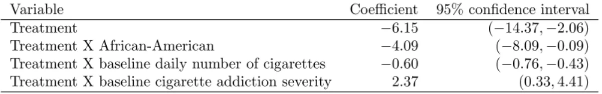
To get an estimate of SATE, we fit a linear model for the outcome that includes treatment condition and all the baseline covariates in Table 1. Consistent with findings by Reid and colleagues, we find a sig-nificant average decrease of ten cigarettes a day as a result of the treatment. We then explore treatment effect heterogeneity, considering models with the same variables (as main effects) plus covariate-treatment interactions. For model selection, we use stepwise regression with forward selection and backward elimi-nation, minimizing the Akaike information criterion. The model selected, presented in Table 2, includes interaction terms of treatment with African-American race cateogory, baseline number of cigarettes per day, and with baseline cigarette addiction severity. Specifically, African-American participants and participants who smoked a larger number of cigarettes per day at baseline experienced a larger reduction, and those with higher baseline addiction score experienced a smaller reduction, in cigarettes smoked per day.
A key problem with trying to genearlize the RCT results to the target population is that the baseline cigarette addiction severity score is a treatment effect moderator, but its target population distribution is unknown, because this variable is not available from the NSDUH. The methods described in this paper can be used to generate TATE estimates accounting for possible distributions of cigarette addiction severity in the target population. In the RCT, the mean of this variable is 4.05 (on a 1 to 5 scale). We assume that the mean cigarette addiction severity score in the target population is somewhere between 3 and 5, and let this sensitivity parameter vary over this range. Applying the outcome-model-based method described in section3.1.1, we have TATE ranging from−9.87, 95% CI (−12.51,−7.23) (corresponding to mean baseline addiction score 3) to−5.13, 95% CI (−7.98,−2.28) (corresponding to mean baseline addiction score 5).
Table 1: Baseline characteristics of the RCT (n=200) and target population (n=934) samples Target
RCT population
Demographics
Male gender: number (%) 105 (52.5) 587 (62.8) Race/ethnicity: number (%)
White 73 (36.5) 764 (81.8)
African-American 51 (25.5) 67 (7.2)
Hispanic 61 (30.5) 58 (6.2)
Multiple 15 (7.5) 45 (4.8)
Age in years: mean (SD) 42.3 (9.6) 36.9 (12.3) Years of education: mean (SD) 11.5 (2.1)
Employment: number (%)
Full-time 49 (24.5)
Part-time or student 25 (12.5) Retired or unemployed 126 (63.0)
Primary substance abuse
Primary substance of abuse: number (%)
Opiates 113 (56.5)
Cocaine 39 (19.5)
Alcohol/other 48 (24.0)
Severity of primary substance abuse: mean (SD) 0.76 (1.04)
Cigarette smoking and addiction
Daily number of cigarettes: mean (SD) 21.2 (11.3) 17.6 (8.4) Number of smoking years: mean (SD) 26.4 (9.9)
Number of quit attempts: mean (SD) 5.2 (12.6) Urine cotinine: mean (SD) 1209 (667) Addiction severity score: mean (SD) 4.05 (0.78) Withdrawal scale: mean (SD) 1.68 (0.98) SD = standard deviation.
Table 2: Treatment effects from the outcome model with interaction terms Variable Coefficient 95% confidence interval Treatment −6.15 (−14.37,−2.06) Treatment X African-American −4.09 (−8.09,−0.09) Treatment X baseline daily number of cigarettes −0.60 (−0.76,−0.43) Treatment X baseline cigarette addiction severity 2.37 (0.33,4.41)
This model also includes all covariates in Table1as main effects.
and generalized boosted models) and two sets of variables (moderators only and moderators plus other co-variates), we find that the weights generated from the logistic sample membership based on the combination of moderators and covariates observed in both samples (race, baseline cigarettes per day, age and gender) result in the best balance, for the moderators as well as the other covariates. Specifically, these weights reduced the standardized mean differences (between the target population sample and the RCT sample) for all race categories, age and gender to under 0.05; and reduced that for baseline daily number of cigarettes from 0.43 before weighting to 0.15 after weighting.
Using these weights, we fit the same outcome model with interactions to the weighted RCT sample; results are presented in Table3. The coefficients of the interaction terms are similar to those from the unweighted model in Table 2, but their confidence intervals are wider due to the weighting. Applying the
Table 3: Treatment effects from the weighted outcome model with interaction terms Variable Coefficient 95% confidence interval Treatment −3.70 (−17.13,9.72) Treatment X African-American −4.49 (−8.11,−0.87) Treatment X baseline daily number of cigarettes −0.55 (−0.82,−0.27) Treatment X baseline cigarette addiction severity 1.77 (−1.77,5.30)
This model was fit to RCT data weighted to adjust for the differential distribution of race, gender, age and baseline daily number of cigarettes between the two samples. The
model includes all covariates in Table1as main effects.
Figure 2: Results of the outcome-model-based and weighted-outcome-model-based sensitivity analyses with the data application.
3.0 3.5 4.0 4.5 5.0
−15
−10
−5
0
sensitivity parameter: mean addiction score in target population
T
A
TE (95% confidence bound)
outcome−model−based sensitivity analysis
weighted−outcome−model−based sensitivity analysis
outcome-model-based sensitivity analysis, we have TATE ranging from−8.36, 95% CI (−12.50,−4.23) (cor-responding to mean baseline addiction score 3) to −4.83, 95% CI (−8.76,−0.90) (corresponding to mean baseline addiction score 5).
Figure2includes the ranges of TATE with confidence bounds from both the sensitivity analyses presented here. These ranges are below zero, suggesting that this smoking cessation intervention, if applied to the target population, would result in smoking reduction. These results are generally consistent with the RCT findings, but give us more confidence in what the effects would be among the target population of cigarette smokers among people seeking alcohol/drug use treatment in the US.
6
Discussion
there are variables that moderate treatment effect, but some of those variables (V) are not available from the data they have for the target population. For this case, we offer an outcome-model-based method, a method fully based on weighting, and a weighted-outcome-model-based method which combines elements of the first two. The two methods based on the outcome model are relatively straightforward and only requires specifying a plausible range for the mean of V in the target population; the weighting-based method is complicated and thus is recommended only for the case with binary moderators.
The second situation is when researchers are concerned that there may be treatment effect heterogeneity that is not detected given the observed variables in the RCT, and ask what that implies about TATE. Here we consider a composite variableU that represents the remaining effect moderation factors after accounting for the observed moderators (and possibly other covariates). For this case, we offer a bias-formula-based method and a weighting-plus-bias-formula-based method. With both methods, we vary two parameters, one representingU’s association with being in the RCT, the other representing its moderation effect, and determine how TATE estimates change as a function of these parameters.
In this paper, we consider the RCT and the target population samples as disjoint sets. The proposed methods, however, are easily adapted to the situation where the RCT sample is a subset of the target population sample. In that caseS = 1 denotes being in the RCT, but all individuals (withS= 1 orS= 0) are in the target population sample. All quantities regarding the target population are not conditioned on
S = 0. The weighting procedures involve modeling S using the target population sample (which includes RCT subjects), and weighting RCT subjects by the inverse of their probability of being in the RCT.
There are several directions for future extension of these sensitivity analyses. First, these methods apply when we do not have outcome data for the target population. There are, however, situations where the outcome under control or a combination of outcome under control and treatment for different individuals is observed in the target population. Currently, methods exist that use target population outcome data under control, but only for generalization where all data, including moderating variables, are observed [Kern et al.,
2016]. The proposed methods could be adapted to incorporate target population outcome data.
Second, the proposed methods that use weighting are based on a specific method of adjusting treatment effect estimates for the differential distribution of a moderator—adjustment by weighting. Another adjust-ment strategy is to fit a flexible model of the outcome as a function of treatadjust-ment, covariates and interaction terms, and either impute potential outcomes for individuals in the target population as the basis to esti-mate TATE, or estiesti-mate treatment effects for covariate strata and average these estiesti-mates using the target population covariate distribution [seeKern, Stuart, Hill, and Green,2016, for example]. Future work should investigate ways to extend the sensitivity analysis procedures we present here to that approach.
Third, the proposed methods do not cover the case where researchers are concerned about a specific vari-able (e.g., parents’ education attainment) that is known or suspected (based on prior evidence) to moderate treatment effect, but is not measured by the RCT. Methods forU do not apply as the moderator in this case is a specific variable, not the remaining composite moderator. This situation is related to our first situation with a specific moderator V, except that this variable is not measured in the RCT. Future investigation is needed to extend our first set of proposed methods to this situation, perhaps using a combination of additional assumptions and external information about this variable.
Fourth, the proposed outcome-model- and bias-formula-based methods assume a linear model for the potential outcomes. In the case of a binary outcome, for example, this means assuming treatment affects the outcome on the risk difference scale. Recent work byDing and VanderWeele[2015] shows that for a binary outcome, effects measured on the odds ratio scale tend to be less heterogenous than on the risk difference (and also risk ratio) scale. One of our next steps is to adapt these sensitivity analysis methods to effect scales that are less heterogeneous for specific outcomes, for example odds ratio for a binary outcome and rate ratio for a count outcome.
To conclude, in this paper we have presented methods for assessing sensitivity of results regarding gen-eralizability of treatment effects to effect heterogeneity on unobserved characteristics. These methods are helpful to researchers and policy makers who are interested in the effect of a treatment for a certain popu-lation, given the common situation that not all effect moderators are measured both in the RCT and in the target population.
References
Onyebuchi a Arah, Yasutaka Chiba, and Sander Greenland. Bias formulas for external adjustment and sensitivity analysis of unmeasured confounders. Annals of epidemiology, 18(8):637–46, 2008. doi: 10. 1016/j.annepidem.2008.04.003.
Stephen R. Cole and Elizabeth A. Stuart. Generalizing evidence from randomized clinical trials to target populations: The ACTG 320 trial. American Journal of Epidemiology, 172(1):107–15, jul 2010. doi: 10.1093/aje/kwq084.
J. Cornfield, W. Haenszel, E. C. Hammond, A. M. Lilienfeld, M. B. Shimkin, and E. L. Wynder. Smoking and lung cancer: Recent evidence and a discussion of some questions. Journal of the National Cancer Institute, 22:173–203, 1959.
Peng Ding and Tyler J. VanderWeele. Generalized Cornfield conditions for the risk difference. Biometrika, 101(4):971–977, 2014. doi: 10.1093/biomet/asu030.
Peng Ding and Tyler J. VanderWeele. The differential geometry of homogeneity spaces ccross effect scales. ArXiv: 1510.08534v2. 2015.
Peng Ding and Tyler J. VanderWeele. Sensitivity analysis without assumptions. Epidemiology, 27(3):368– 377, 2016. doi: 10.1097/EDE.0000000000000457.
Joseph L Gastwirth, Abba M Krieger, and Paul R Rosenbaum. Dual and simultaneous sensitivity analysis for matched pairs. Biometrika, 85(4):907–920, 1998.
Joel B Greenhouse, Eloise E Kaizar, Kelly Kelleher, Howard Seltman, and William Gardner. Generalizing from clinical trial data: A case study. The risk of suicidality among pediatric antidepressant users. Statistics in Medicine, 27:1801–1813, 2008. doi: 10.1002/sim.
S Greenland. Basic methods for sensitivity analysis of biases. International Journal of Epidemiology, 25(6): 1107–1116, 1996. doi: 10.1093/ije/25.6.1107.
Guanglei Hong. Ratio of mediator probability weighting for estimating natural direct and indirect effects. Proceedings of the American Statistical Association, Biometrics Section, pages 2401–2415, 2010.
Holger L. Kern, Elizabeth A. Stuart, Jennifer L Hill, and Donald P. Green. Assessing methods for generalizing experimental impact estimates to target samples. Journal of Research on Educational Effectiveness, 9(1): 103–127, 2016. doi: 10.1080/19345747.2015.1060282.
Robert B Olsen, Larry L Orr, Stephen H Bell, and Elizabeth A Stuart. External validity in policy evaluations that choose sites purposively. Journal of Policy Analysis and Management, 32(1):107–121, 2013. ISSN 15206688. doi: 10.1002/pam.21660.
Malcolm S Reid, Bryan Fallon, Susan Sonne, Frank Flammino, Edward V Nunes, Huiping Jiang, Eva Kuoniotis, Jennifer Lima, Ron Brady, Cynthia Burgess, Eric Pihlgren, Louis Giordano, Aron Starosta, James Robison, and John Rotrosen. Smoking cessation treatment in community-based substance abuse rehabilitation programs. Journal of Substance Abuse Treatment, 35(1):68–77, 2008.
P R Rosenbaum. Sensitivity analysis for certain permutational inferences in matched observational studies. Biometrika, 74:13–26, 1987.
Paul R Rosenbaum and Donald B Rubin. Assessing sensitivity to an unobserved binary covariate in an observational study with binary outcome. Journal of the Royal Statistical Society, 45(2):212–218, 1983a. Paul R Rosenbaum and Donald B Rubin. The central role of the propensity score in observational studies
Sebastian Schneeweiss. Sensitivity analysis and external adjustment for unmeasured confounders in epidemi-ologic database studies of therapeutics. Pharmacoepidemiology and Drug Safety, 15:291–303, 2006. doi: 10.1002/pds.1200.
Elizabeth A Stuart and Anna Rhodes. (In press). Generalizing treatment effect estimates from sample to population: A case study in the difficulties of finding sufficient data. Evaluation Review.
Elizabeth A Stuart, Stephen R Cole, Catherine P Bradshaw, and Philip J Leaf. The use of propensity scores to assess the generalizability of results from randomized trials. Journal of the Royal Statistical Society: Series A (Statistics in Society), 174(2):369–386, 2011. doi: 10.1111/j.1467-985X.2010.00673.x.
Elizabeth A. Stuart, Catherine P. Bradshaw, and Philip J. Leaf. Assessing the generalizability of ran-domized trial results to target populations. Prevention Science, 16(3):475–485, 2015. doi: 10.1007/ s11121-014-0513-z.
Ryoko Susukida, Rosa M Crum, Elizabeth A Stuart, Cyrus Ebnesajjad, and Ramin Mojtabai. Assessing sample representativeness in randomized controlled trials: Application to the National Institute of Drug Abuse Clinical Trials Network. Addiction, 2016. doi: 10.1111/add.13327.
E. Tipton. Improving generalizations from experiments using propensity score subclassification: Assump-tions, properties, and contexts. Journal of Educational and Behavioral Statistics, 38(3):239–266, 2013. doi: 10.3102/1076998612441947.
Tyler J Vanderweele and Onyebuchi a Arah. Bias formulas for sensitivity analysis of unmeasured confounding for general outcomes, treatments, and confounders. Epidemiology, 22(1):42–52, 2011. doi: 10.1097/EDE. 0b013e3181f74493.
Herbert I Weisberg, Vanessa C Hayden, and Victor P Pontes. Selection criteria and generalizability within the counterfactual framework: Explaining the paradox of antidepressant-induced suicidality? Clinical Trials, 6(2):109–118, 2009. doi: 10.1177/1740774509102563.
Acknowledgements
TQN is supported by NIDA grant T32DA007292 (PI: Renee M. Johnson). EAS and CE are supported by NSF grant DRL-1335843. We thank Ryoko Susukida and Ramin Mojtabai for their kind support for our search for an appropriate data example.