Gonzalez_unc_0153D_16174.pdf

S

M

C

D

C

Robert M. Gonzalez

A dissertation submitted to the faculty of the University of North Carolina at Chapel Hill in par-tial fulfillment of the requirements for the degree of Doctor of Philosophy in the Department of

Economics.

Chapel Hill 2016

Approved by:

Klara Peter

Patrick Conway

Erica Field

David Guilkey

c

ABSTRACT

ROBERT M. GONZALEZ: Social Monitoring and Corruption in Developing Countries. (Under the direction of Klara Peter)

This dissertation studies the impact of social monitoring–monitoring of government officials by ordinary citizens–on institutional corruption. Specifically, I study a monitoring initiative in which citizens used cell phones to report instances of fraud during the 2009 Afghan presidential election. Since implementation of the program required cell phone coverage, I combine cover-age maps with unique data on the geographic location and fraud levels of polling centers across Afghanistan to determine: (i) the effect of coverage on fraud, and (ii) whether social monitoring is the main corruption-deterring mechanism among several competing channels. Using a spatial regression discontinuity (RD) design along the cell phone coverage boundary, I find considerable evidence that cell phone-based participation deters corrupt behavior. Polling centers inside cell phone coverage areas report up to a 26 percent drop in the share of fraudulent votes relative to cen-ters outside. Analyses of the effect of coverage on election-related violence and the tribal composi-tion of villages suggest that the observed declines in fraud cannot be attributed to these alternative channels. From a policy perspective, these results illustrate how a widespread technology, namely cell phones, can exert a positive externality on institutional development via corruption deterrence.

ACKNOWLEDGMENTS

This dissertation was made possible by an incredible group of mentors: Patrick Conway, Erica Field, David Guilkey, Klara Peter, and Tiago Pires. I owe my deepest gratitude to my advisor Klara Peter for her unconditional support and guidance. Emulating her dedication and work ethic has made me a better researcher. I thank Patrick Conway for always providing a thoughtful critique. I am deeply indebted to Erica Field for believing in me and for instilling in me, through her teachings and collaboration, a profound passion for the field of Development Economics. David Guilkey is one of the best teachers I have had in my life. I thank him for laying the foundation of my knowledge of Econometrics. Lastly, I thank Tiago Pires for dedicating countless times to read and review my work, but above all, for being a friend and always being there to listen.

I am also grateful to have found great support from individuals outside of my committee. I specially thank Donna Gilleskie for her always thoughtful advice and for making me a better writer and economist. I thank Helen Tauchen for both, insightful comments on my work and for helping me navigate the stressful graduate school process. I am indebted to faculty and fellow students in the UNC Applied Micro group for listening and commenting on my work from its very early stages.

TABLE OF CONTENTS

LIST OF TABLES . . . vii

LIST OF FIGURES . . . viii

1 Introduction . . . 1

2 Background . . . 7

2.1 The 2009 Afghan Election . . . 7

2.2 The Audit and Recount . . . 9

3 Theoretical Framework . . . 11

3.1 The Transmitter’s Problem . . . 11

3.2 The Election Official’s Problem . . . 12

3.3 The Candidate’s Problem . . . 13

4 The Effect of Coverage on Fraud . . . 16

4.1 Data and Variables . . . 16

4.1.1 Measures of fraud . . . 16

4.1.2 Cell phone coverage . . . 17

4.1.3 Polling Center Characteristics . . . 18

4.2 Empirical Framework . . . 21

4.2.1 Regression Discontinuity Design (RD) . . . 21

4.2.2 Validity of the RD Identifying Assumptions . . . 25

4.3 Results . . . 31

4.3.1 Graphical Analysis . . . 31

4.3.2 One-Dimensional RD . . . 32

4.3.3 Boundary RD . . . 35

4.4 Robustness Checks . . . 38

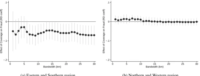
4.4.1 Boundary Sensitivity . . . 39

4.4.2 Bandwidth Choice and Polynomial Order . . . 40

4.4.3 Sensitivity of Results to Inclusion of Covariates . . . 41

5 Alternative Channels of Fraud . . . 43

5.1 Election-related Insurgent Violence . . . 43

5.2 Voter’s Affinity . . . 47

6 Conclusion and Discussion . . . 51

A The Audit and Recount Process . . . 53

B Model Extensions . . . 55

B.1 Nonlinear Reporting Cost Function . . . 55

B.2 Free-riding and Fraud Reporting . . . 55

B.3 The Voter’s Problem . . . 56

B.4 Two Candidates . . . 57

C Additional Figures and Tables . . . 61

LIST OF TABLES

4.1 Mean Comparison for Various Polling Center Characteristics . . . 26

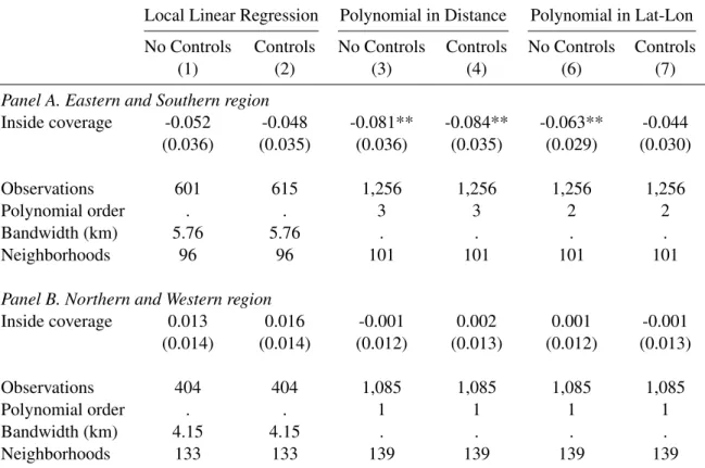
4.2 Average Effect of Mobile Coverage on Category C+ Fraud (Scalar RD) . . . 34

4.3 Averaged Conditional Treatment Effects (Category C+ fraud) . . . 38

4.4 Sensitivity of Results to the Addition of Baseline Covariates . . . 42

C.1 Sample and Imputations . . . 69

C.2 Mean Comparison for Various Polling Center Characteristics . . . 70

C.3 Tribes and Tribal Confederations (Southeast Afghanistan) . . . 72

LIST OF FIGURES

2.1 Total Votes and Vote Percentage Received by Top Two Candidates . . . 10

4.1 Mobile 2G Coverage and Polling Centers . . . 19

4.2 Histograms and Densities of the Forcing Variable . . . 30

4.3 Binned Averages for Category C+ fraud (RD plot) . . . 32

4.4 Spatial Distribution of Boundary Treatment Effects ( Category C+ fraud) . . . 36

4.5 Distribution of Boundary Treatment Effects ( Category C+ fraud) . . . 38

4.6 Sensitivity of Results to Bandwidth Choice (Category C+ fraud) . . . 40

4.7 Sensitivity of Results to Polynomial Order (Category C+ fraud) . . . 41

5.1 Insurgent Attacks on Election Day . . . 44

5.2 Spatial Distribution of Boundary Treatment Effects for Various Indicators of Violence 47 5.3 Major Tribal Confederations, Southeast Afghanistan . . . 49

5.4 Spatial Distribution of Boundary Treatment Effects: Ghilzai Pashtun village . . . . 50

C.1 Binned Averages for Various Covariates (Covariate RD Plots) . . . 61

C.2 Afghan Provinces and Regions . . . 64

C.3 Polling Center Density Estimates . . . 64

C.4 All Casualties (Jan, 2009 - Sept, 2009) . . . 65

C.5 Afghan villages, 2012 . . . 65

C.6 Tribal Map, Kandahar Province . . . 66

C.7 Sample Reporting Cost Function . . . 67

LIST OF ABBREVIATIONS

2G Second Generation

ACTE Averaged Conditional Treatment Effects

AIMS Afghanistan Information Management Services

CTE Conditional Treatment Effects

ECC Electoral Complaints Commission

GIS Geographic Information System

GPS Global Positioning System

GSM Global System for Mobile Communications

IEC Independent Election Commission

MISTI Measuring Impacts of Stabilization Initiatives

NASA National Aeronautics and Space Administration

RD Regression Discontinuity

SRTM Shuttle Radar Topography Mission

CHAPTER 1

INTRODUCTION

Corruption is widely presumed to have a large detrimental effect on economic growth. There is evidence that corruption decreases competition and investment, dampens government revenue, and obstructs the delivery of government services (Mauro (1995), Svensson (2005), Olken and Pande (2012)).1 One theory is that corruption flourishes in settings in which citizens are particularly dis-enfranchised. This has motivated policy interventions to strengthen community efforts to engage in monitoring of public officials as a means of combating corruption.

In theory, bolstering grassroots monitoring may be more effective in reducing corruption than increasing external monitoring efforts, particularly at very high levels of corruption where auditors can readily be bought out.2 _{Meanwhile, social monitoring may have little potential when} com-munity members lack a means of directly punishing corrupt officials or face immediate threats of retribution. Thus far, the empirical evidence has been mixed. Olken (2007) and Banerjee, Banerji, Duflo, Glennerster, and Khemani (2010) find little support for the idea that increasing community monitoring results in better behavior of public officials, while Bjorkman and Svensson (2009) find that government performance improves significantly when community members engage in active surveillance. One key ambiguity is that the intervention found to be effective took a very inten-sive (and expeninten-sive) approach to fostering community participation, leaving open the question of whether scalable community monitoring efforts have the potential to make a difference.

This paper provides evidence that they do. I show that a simple approach to strengthening

1_{Corruption in Afghanistan, the country studied in this paper, is so pervasive that in 2013, Transparency}

Interna-tional ranked it as the world’s most corrupt country (Transparency InternaInterna-tional 2013), while American authorities argue that corruption, and not the Taliban, is the main existential threat to this country (Riechmann 2014).

2_{Throughout the paper I conceptualize social monitoring as a mechanism by which ordinary citizens can better}

social monitoring capacity via cell phone hotlines can be highly effective in reducing corruption. Hotlines create a direct means of reporting fraud through a widely available medium – mobile phones.3 The advent of cell phones in the developing world make this approach particularly ger-mane. Mobile connectivity rates have increased exponentially in the developing world over the past decade, giving rise to a host of potential interventions that rely on cell phones as the primary medium for citizens to monitor and report corrupt behavior.4

I investigate the impact of social monitoring on corrupt behavior in the context of a United Nations (U.N.)-led monitoring initiative that created election fraud hotlines to facilitate fraud re-porting by ordinary citizens during the 2009 Afghan presidential election. Since implementation required cell phone coverage, I identify the causal effect of social monitoring by exploiting geo-graphic variation in the areas where social monitoring was feasible based on cell phone coverage availability. Using a spatial regression discontinuity (RD) design that compares polling centers within a close distance of the cell phone coverage boundary, I examine the effect of mobile phone coverage – and hence the potential threat to a misbehaving official induced by greater social mon-itoring – on election fraud.

The empirical analysis employs several novel data sources, including (1) detailed coverage maps based on the location of cell phone towers of the two largest mobile service providers in Afghanistan;5(2) data on the precise location of polling centers collected by International Security Assistant Force (ISAF) inspection teams shortly after the election;6 and (3) polling center level data on various measures of election fraud collected by a U.N.-sponsored audit shortly after the election.

My results indicate that cell phone coverage reduces corruption, and social monitoring is the

3_{According to the International Telecommunication Union (ITU), the cell phone penetration rate in Afghanistan}

was close to 40 subscribers per 100 people in 2009. By 2013, this number had risen to 71 (ITU 2015).

4_{For a detailed description of the history and growth of ICT-based electoral monitoring refer to Schuler (2008).}

5_{I obtain these data fromCollins Bartholomew, which represents the GSMA, an association of major GSM mobile}

service providers around the world. Cell phone service providers supply coverage data directly to the GSMA.

6_{Geolocation data were provided by the Afghan Independent Election Commission (http://www.iec.org.af)}

primary mechanism through which this occurs. For polling centers within a 5 to 6 kilometer bandwidth around the coverage boundary, the share of fraudulent votes in centers inside cover-age areas is about 26 percent lower relative to centers outside. The results are robust to several choices of bandwidth and polynomial order. To assess the validity of the RD design, I investigate whether other polling center characteristics change discontinuously at the boundary. In particular, I compare 28 electoral, geographic, socioeconomic, and demographic indicators for villages and settlements where polling centers are located. The results indicate a smooth transition across the coverage boundary and thus little evidence that changes in fraud at the boundary are explained by changes in these indicators. To the best of my knowledge, this is the first study to provide evidence on the impact of cell phone coverage on institutional corruption.

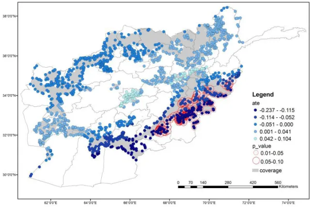
To explore the spatial heterogeneity of the results, I modify and implement a recently-developed boundary RD design that estimates treatment effects at various points along the two-dimensional coverage boundary.7 _{Since the method recovers a distribution of treatment effects along the} bound-ary, one can determine the areas or sections of the boundary where fraud is more responsive to social monitoring. The results suggest significant spatial heterogeneity in the effect both across and within regions of Afghanistan. Economically and statistically significant drops in fraud at the coverage boundary are present in the eastern and southern regions of the country whereas aver-age impacts in the northern and western regions are close to zero in magnitude and statistically insignificant.

Fraud may respond to cell phone coverage for reasons other than social monitoring. I use an illustrative theoretical model to motivate which channels to explore. In particular, I specify a classical supply and demand model where votes can be bought legally (via advertising, campaign promises, etc.) or illegally. In the case of illegal/fraudulent votes, corruption takes the form of collusion between polling center managers (suppliers of votes) and the corrupt candidates (de-manders of votes). The price of fraudulent votes is a function of social monitoring.8 Given the

7_{I employ a modification of the boundary RD method proposed by Imbens and Zajonc (2011).}

high incidence of election-related violence, the price of legal votes is a function of both voters’ affinity towards the candidates and the likelihood that the polling center is attacked by insurgents. Higher levels of expected violence require a higher price to guarantee that constituents vote. Cov-erage enters the model as a shifter in the probability of social monitoring and, hence, a shifter in the equilibrium quantity of fraudulent votes. However, the price of legal votes, and hence the equilibrium level of fraud, may also shift with coverage if the likelihood of insurgent attacks or voters’ affinity depends on coverage.9 _{Therefore, these two channels may lead to changes in the} equilibrium level of fraud that mimic the social monitoring effect.

First, I examine whether political violence by insurgent groups, which is strongly related to both cell phone coverage (Shapiro and Weidmann 2013) and electoral fraud (Callen and Weidmann 2013), confounds the social monitoring effect. I replicate the spatial RD analysis using recently declassified data on daily insurgent and IED attacks, along with data on civilian and military casu-alties around election day.10 _{Using the boundary RD design, I test whether the violence outcomes} change discretely at points in the coverage boundary where I observe significant changes in fraud as well. Results suggest that the treatment effects of coverage on violence are generally small in magnitude and statistically insignificant for most points in the boundary. This has key implications for the identification of the social monitoring effect since drops in fraud at the boundary cannot be explained by significant drops in violence outcomes. With this in mind, a secondary, yet important contribution of this paper is to advance our understanding of the relationship between cell phone access and insurgent violence.

Second, given the importance of tribal loyalty in Afghan society, I also test directly whether the boundary effects are confounded by discrete changes in the tribal composition of villages, a strong predictor of party affiliation.11 _{To explore this possibility, I georeference detailed tribal}

9_{For instance, if the likelihood of violence or voters’ affinity drops with coverage, legal votes become less costly.}

Thus the candidate substitutes fraudulent with legal votes.

10_{Data on IED attacks are obtained from Shaver and Wright (2015) and refer to SIGACTs or Significant Actions.}

These data are collected directly by the military and constitute the official database of insurgent attacks. Data on civilian and military casualties are provided by the Worldwide Incident Tracking System (WITS 2009).

11_{This might be the result, for instance, of cell phone providers giving preference to certain ethnic groups by}

maps collected by the Culture and Conflicts Studies program containing information on the geo-graphic distribution of more than 50 tribes and ethnic groups across Southeastern Afghanistan.12 I then combine the georeferenced maps with village location data from the Measuring Impacts of Stabilization Initiatives project (MISTI 2013) to construct village-level indicators of primary tribe and tribal confederation for almost 18,000 villages. I replicate the boundary RD analysis for portions of the boundary where there seem to be changes in the number of villages belonging to the same tribal confederation as the main candidates. I show that, while there is some evidence of changes in the tribal structure of villages at certain points along the boundary, these changes cannot explain the observed drops in fraud as there is no substantial overlap in the boundary points where both tribal affiliation and fraud change sharply.

This paper contributes to a growing effort to understand the effectiveness of grassroots moni-toring on illegal behavior within the realm of election fraud. Callen and Long (2015) implement a field experiment where individuals record photographs of the total vote tally at randomly selected polling centers during the 2010 Afghan parliamentary election. This monitoring technology, how-ever, is conceptually different from the one I study in this paper as it does not necessarily rely on cell phone coverage. Further, the monitoring is performed by a select group of individuals rather than all voters. Aker, Collier, and Vicente (2014) explore the impact of an SMS hotline during the 2009 Mozambican election, a monitoring technology that is very similar to the Afghan setting. However, while they show convincing evidence that the hotline lowers fraud levels, it is not clear whether this result would hold in a fragile security environment like Afghanistan. Prior to the election, the Taliban issued several warnings targeting polling centers and voters while on election day the number of attacks exceeded the 2009 daily average by a factor of seven.13 _{In such cases,} election-related violence hampers monitoring incentives as individuals fear retaliation or are sim-ply unable to witness fraud if not present at the polling centers. The fact that I find significant drops

expanding coverage into their locations.

12_{The Culture and Conflicts Studies program is part of the Naval Postgraduate School.}

13_{Figures calculated by author using SIGACTs data obtained from Shaver and Wright (2015). The average number}

in fraud at the coverage boundary suggests that monitoring technologies that offer some degree of plausible deniability to potential whistleblowers can be effective even in settings characterized by extreme political violence.14

This study is also novel in providing rigorous evidence on the role of information and com-munications technologies (ICT) on improving information transfer and social monitoring capacity. This is a particularly important contribution given the rapid expansion in mobile services expe-rienced in the developing world throughout the last decade.15 _{More generally, the results in this} paper show how commonly available communication devices, such as cell phones, can exert a positive externality on institutional development. In that sense, the results add to a rapidly advanc-ing literature on the effectiveness of ICT-based policies on improvadvanc-ing transparency and economic development outcomes in general (e.g., Jensen (2007), Aker (2010), and Aker et al. (2014)).

Lastly, from an empirical standpoint, this paper contributes to the literature on spatial and, more specifically, geographic RD (e.g., Imbens and Zajonc (2011), Keele and Titiunik (2013)). A literature that is rapidly growing as advances in GPS technology are increasing the availability of micro-level geospatial data. More importantly, however, is that it illustrates an empirical frame-work that can be used by other studies trying to uncover heterogeneous effects of mobile phone coverage on any outcome variable using a spatial framework. Further, the possibility of obtaining spatially heterogeneous effects along a geographic boundary has key policy implications as it can guide agencies in the design of localized anti-corruption policies.

The paper is structured as follows: Chapter 2 provides a background of the Afghan 2009 presi-dential election as well as the nationwide audit that followed shortly afterwards. Chapter 3 presents the theoretical framework. Chapter 4 describes the empirical method and reports results of the ef-fect of coverage on fraud. Chapter 5 explores alternative channels of fraud. Lastly, Chapter 6 concludes.

14_{See Chassang and Padro-i-Miquel (2014) for a detailed treatment on the importance of plausible deniability to}

incentivize monitoring and to avoid side-contracting between monitors and misbehaving agents.

15_{In the case of Afghanistan, for instance, the number of mobile subscribers rose from 1.7 million in 2006 to around}

17.1 million in 2012. This translates into a mobile penetration (number of subscribers per 100 inhabitants) of 6.27 in 2006 and 63.3 in 2012

CHAPTER 2

BACKGROUND

This chapter provides a detailed description of the 2009 Afghan presidential election and of the audit and recount process that took place shortly after the election.

2.1 The 2009 Afghan Election

The 2009 Afghan presidential election marked the second election after the toppling of the Tal-iban regime in 2001. Fraud allegations during the 2004 presidential election led to the creation of the Electoral Complaints Commission (ECC) precisely to investigate and adjudicate fraud related complaints for the upcoming 2009 presidential election. This constituted the first time in Afghan history that a formal channel for individuals to report electoral complaints was created. In addition to adjudication of complaints, the ECC was given the power to issue audits, recounts, and runoff elections if necessary (Electoral Complaints Commission 2010). To improve transparency and guarantee independence from the executive power, three of the five appointed ECC commission-ers (including the chairman) were international experts directly appointed by the United Nations Representative of the Secretary General. The two Afghan commissioners were selected from the Afghanistan Independent Human Rights Commission and the Supreme Court(National Democratic Institute 2010).

to the ECC in case a follow-up investigation would take place. The ECC, however, guaranteed this information was not to be disclosed. These hotlines were widely publicized through a public out-reach program that included television and several radio advertisements in both Pashto and Dari.1 Similarly, instances of violence, intimidation at the polling center, and corruption in general could be reported to the 119 Afghan corruption hotline led by the European Union Police Mission in Afghanistan (EUPOL) and relatively known by the Afghan population.2 _{Private organizations also} encouraged the use of cell phones to report instances of fraud. For example, in the weeks prior to the election, Pajhwok News, a major independent news agency in the country, along with other international NGOs, enabled several hotlines. In addition the agency deployed around 80 reporters around the country who were instructed to use their mobile phones to text and call in incidents of violence and fraud (Himelfarb 2010).

Allegations of fraud during the 2009 Afghan election were widespread.3 According to ECC’s chairman Grant Kippen, the agency received more than 3,300 complaints with close to 80 per-cent of these complaints received during the polling and counting period (Electoral Complaints Commission 2010). In terms of the types of complaints, most complaints–about 47 percent–dealt with polling and counting irregularities, followed by complaints on intimidation, and violence at the center (about 26 percent). The remaining types of complaints were distributed between: ac-cess to stations (11 percent), missing election materials at the center (4 percent), and other types (12 percent). This degree of citizen participation represented a major improvement from the 2004 presidential election when no formal channel to file claims existed. A direct implication of this was the implementation of a nationwide audit that is discussed in detail in the following section.

1_{More information on the hotlines as well as the public outreach program can be found at the ECC’s official website}

www.ecc.org.af

2_{According to a 2012 UNDP survey cited by the Ministry of Interior Affairs (MOIA), about 80-90 percent of the}

Afghan population has some familiarity with the police hotline. This information was obtained by the author through an interview with MOIA representatives.

3_{Refer to Panels (b), (c), and (d) in Appendix Figure C.8 for examples of typical fraudulent activities.}

2.2 The Audit and Recount

Election day took place on August 20, 2009. Eighteen days after the tallying of votes began; the ECC ordered a nationwide audit of polling stations after initial investigations of the received complaints revealed clear evidence of widespread fraud.4 The audit called for the investigation of polling stations reporting unusually high turnout and an unusually high majority of votes for a single candidate. Specifically, the audit-triggering criteria were: (1) stations in which 600 or more votes were cast, (2) stations in which one candidate received 95 percent or more of the total votes cast, and (3) stations satisfying both (1) and (2). The ECC referred to each of these categories as Category A, B, and C, respectively.5

The motivation for these criteria lied primarily in the particular design of the election and the unusual pattern of reported total votes per station. In particular, polling station managers were pro-vided with a ballot book containing exactly 600 empty ballots (Electoral Complaints Commission 2010).6 However, a significant number of stations reported totals of exactly 600 or more votes cast. This was particularly unusual given the overall low turnout across the country resulting from the fragile security environment (Khadhouri 2010). Such discrepancies in reported turnout can be clearly seen in Figure 2.1a which shows a histogram of total votes cast per station for the top two candidates. Notice the pronounced jump in the frequency of total votes cast at exactly 600 for candidate Hamid Karzai in particular.7 The incidence of stations where a candidate obtained more than 95 percent of the total vote share was equally unusual. Note in Figure 2.1b that a substantially high number of stations (with more than 100 total votes cast) had exactly 100 percent vote share

4_{For reference, a polling station is a physical location within a polling center. In the sample studied, the average}

number of polling stations per center is about 4 with some centers having up to 20 stations.

5_{To be more specific the ECC defined a total of six categories, however, given the similarity between some of the}

categories I reduce them to three aggregate categories. Refer to Appendix A for a more detailed explanation of the audit categories.

6_{Refer to Panel (a) of Appendix Figure C.8 for a sample ballot booklet.}

7_{Also notice similar, although not as pronounced, peaks at various multiples of 50 starting with 200. See Beber}

for a single candidate (particularly Karzai).

0 200 400 600 800 1000

Frequency

0 100 200 300 400 500 600 700 800 900 1000 Total votes per polling station

Karzai Abdullah

(a) Total votes (per polling station)

0 500 1000 1500

Frequency

0 .2 .4 .6 .8 1

Percentage of votes received by candidate Karzai Abdullah

(b) Percentage votes received (per polling station)

Figure 2.1: Total Votes and Vote Percentage Received by Top Two Candidates

Notes:Frequency of total votes received by the top two candidates at the station level. Sample restricted to stations

where candidates obtained more than zero votes. Bar width is 1. In panel (b), sample is restricted to stations where a candidate obtained a positive share and to stations were 100 or more total votes were cast. Bar width is 0.01.

The ECC classified 3,376 stations, or nearly 15 percent of all stations, as potentially fraudulent (i.e., falling in one of the three fraud categories mentioned above). Ultimately, the ECC performed a partial audit of all suspect stations given the need to determine, in a timely manner, whether a runoff election was needed. Particularly, 10 percent of the qualifying stations were randomly selected for a thorough investigation. From the inspected stations, the ECC created a “fraud co-efficient” for each of the three categories described above. In essence, the fraud coefficients are the percentage of votes found to be fraudulent out of the total votes inspected within the category. Some indicators of fraud were: ballot boxes with broken or tampered seals, uniform markings in most ballots, discrepancies in tally sheets and box totals, etc.

On October 18, nearly two months after election day, the ECC released the results of the audit. Once suspect votes were eliminated from the count, Hamid Karzai’s vote share dropped from 54.6 to 49.67 percent, while the vote share of his main challenger, Abdullah Abdullah, went from 27.8 to 30.59 percent. In lieu of the results, the ECC ordered an immediate runoff election. However, the runoff election did not take place as main challenger Abdullah withdrew from the race.

CHAPTER 3

THEORETICAL FRAMEWORK

The objective of this chapter is twofold: (i) to present a theoretical model that illustrates the link between cell phone coverage and electoral fraud, and (ii) to define channels, other than the social monitoring effect, that may equally affect fraud through coverage. I consider the problem of a candidate determining the purchase of fraudulent and legal votes at a polling center. In the case of fraudulent votes, I follow Callen and Long (2015) by assuming that the candidate pays an upfront price to an election official in charge of a polling center. This price takes into account the possibility that the center is audited as a result of complaints received from individuals at the polling center (i.e., social monitoring). With this in mind, social monitoring enters the model as a shifter in the price of fraudulent votes.1 _{I refer to the individuals reporting fraud as transmitters. The price of} legal votes takes into account the risk of violence that the voters face at the polling place. Higher levels of expected violence require a higher price. Lastly, given the prices of fraudulent and legal votes, the candidate then chooses an optimal level of each to purchase subject to his available campaign funds.

3.1 The Transmitter’s Problem

Consider a polling center servingn voters. Furthermore assume that there exists a nationwide phone hotline to report electoral fraud. Given the widespread use of cell phones (as opposed to fixed-line phones) in the developing world and Afghanistan in particular, suppose individualiuses a cell phone if he decides to report fraud. Reporting fraud carries a physical cost c(D) where

D indicates the accessibility of the medium (cell phones) used to report fraud. In the context of this study D is an indicator for whether the polling center is located in an area with cell phone

1_{In section (3.3) I show that it also has a direct impact on the utility of the candidate as fraudulent votes are dropped}

coverage.2 _{Specifically, let the cost of reporting fraud equalcif the center is on an area with cell} phone coverage (i.e.,D= 1) and¯cotherwise with¯c > c.3

Furthermore, assume that reporting fraud gives i a utility gainλi that can be interpreted as a

“warm glow” parameter ori’s satisfaction from his pro-social behavior. The individual’s net payoff from reporting fraud is therefore given byλi−c(D). He will then decide to report fraud if:

λi ≥c(D) (3.1)

Assumingλi is distributed among voters at the center with probability functionG(λ)then the

probability of an individual making a report given coverage statusDis given byρ(D) = 1−G(D).4

3.2 The Election Official’s Problem

The candidate purchases fraudulent votes from an election official overseeing polling centerj.5 The price of these votes has to guarantee the official’s compliance to sell them.6 _{This price takes} into account the probability that the center is audited as a result of reports by ordinary individuals (i.e., social monitoring). Assume the candidate and the official have perfect information over the distribution ofλiand thus assess that the number of submitted fraud reportsrfollow a random

pro-cess with probability function H(r;n, ρ(D))that takesρ(D)andn as parameters.7 _Furthermore,

2_{In realityDshould indicate whether there is coverage in the area where the individual decides to report fraud (the}

polling center, his house, etc.). This information is unavailable hence I only consider coverage at the polling center. This implicitly assumes that the call to report fraud is made right at the center. However, since centers were located within settlements, it is likely that any calls are made within the “catchment area” of the center so that using the center as a reference in determining coverage should not greatly affect the analysis of the model.

3_{Without loss of generality, I assume that the reporting cost on the non-coverage side ¯c is constant, however,}

this cost might increase as polling center are further away from the coverage boundary. Refer to Appendix B for a discussion of an alternative specification of the reporting cost function that uses a smooth, non-linear function on the non-coverage side.

4_{G(.)is actually a function ofc(D), which in turn, is a function ofD. Refer to Appendix B for an extension of}

Equation 3.1 that considers the possibility of free-riding when reporting fraud.

5_{Although there are other methods for committing fraud, ballot stuffing and manipulation of total counts by officials}

seemed to be the most prevalent for of fraud during the 2009 Afghan election (see Callen and Weidmann (2013))

6_{The offered price must be so that the official’s incentive compatibility constraint binds.}

7_{A possible parameterization forH(.)is a Poisson distribution with the mean rate given byN ρ. In such case, the}

assessed probability that centerjis audited can be written as:P r(r≥¯r) =π(¯r, ρ, N) = 1−P¯r−1

r=0

(N ρ)r_{exp(−N ρ)}

r! .

assume that the center is audited if the number of reportsrexceeds a predetermined thresholdr¯so that the probability that the center is audited is given by:

π(¯r;n, D) = 1−H(¯r;n, ρ(D)) (3.2)

Letting vf, pf, andF denote the number of fraudulent votes, their price, and a marginal fine

respectively, I follow Callen and Long (2015) by assuming that the official faces a lottery in which he expects to be caught with probabilityπ, receive fraud revenuespfvf net of a total finevfF or

succeed with complementary probability1−π and pocket all fraud revenues instead.8 Assuming that the official is an expected income maximizer then the minimum price per fraudulent vote that guarantees compliance to sell fraudulent votes is given by the expression:

π(pfvf −vfF) + (1−π)pfvf = 0

pf =πF (3.3)

where π is obtained from Equation 3.2 and it is assumed that the official receives an offer from only one of the candidates (i.e., payoff from non-compliance is zero).9

3.3 The Candidate’s Problem

The candidate must decide how many votes (both legal and fraudulent) to buy from each center

j. Assume that the auditing agency can differentiate between fraudulent and legal votes so that, once audited, any fraudulent votes are dropped and the candidate only receives legal votesvl. In

case where the center is not audited the candidate simply keeps all votes vl +vf. I consider the

price of legal votes vl to be a function of a parametera that characterizes each village’s affinity

towards the candidate. Villages where the candidate is liked require a lower legal price per vote

8_{I assume that once a fraudulent center is audited, the candidate and polling center manager are penalized.}

There-fore I do not consider any “concealment technology” as in Cremer and Gahvari (1994)

9_{I rely on this assumption to simplify the analysis but also because the pattern observed in the data suggests that}

to entice constituents to vote.10 _{Further, since elections in conflict zones are often characterized} by violence, I also consider the price of legal votes to be a function of an exogenous probability

δthat a violent event takes place at polling center j and as a result the village receives a negative

payoffP. This consideration is particularly important in the Afghan context as the Taliban issued several warnings targeting polling centers and voters on election day (Gall (2009), Filkins (2009)). With this in mind, I define the price of legal votes aspl =f(δ, P, a)with ∂f_∂δ(.) >0, ∂f_∂P(.) >0, and

∂f(.)

∂a <0.

11

Given the assessed probability of an audit in Equation 3.2 and assuming that the candidate has quasilinear preferences over votes, then the maximization problem of the candidate is given by:

max

vl,vf

πvl+ (1−π)

vl+vfα

subject to pfvf +plvl ≤E

where fraudulent votes enter non-linearly (with α ≤ 1) to capture the possibility that fraudulent and legal votes are not perfect substitutes andEis some campaign endowment of the candidate.12 The solution to the problem above provides an optimal relationship between fraudulent votes and their pricepf.13 Substituting the expressions for pricespf andplin order to obtain the equilibrium

level of fraud gives:

vf =

α(1−π)·f(δ, P, a)

πF

_1−α1

(3.4)

Given expressions 3.2 and 3.4 the main prediction of this model is that: Given an increase in the audit probabilityπdue to coverage availability (i.e.,D = 1in Equation 3.2), then the equilibrium

10_{This legal price of votes can be interpreted as advertising costs, campaigning expenditures, etc.}

11_{Refer to Appendix B.3 for an extension of the model that derives an expression for the legal price of votes.}

12_{The quasilinear specification deviates from Callen and Long (2015) perfect substitutes specification. The appeal}

of the quasilinear specification is that it avoids a prediction where the candidate simply substitutes to all fraudulent or all legal votes as soon as the relative price deviates from 1. The studied sample shows a combination of fraudulent and legal votes for the most part not corner solutions like the ones obtained from a perfect substitutes specification.

13_{Recall that the quasilinear specification of the candidate’s utility implies that there might exist a corner solution}

where the candidate only consumes fraudulent votes. More specifically,vf = pEf ifm≥α

−1_pα fE

1−α_{. I consider the}

interior solution only because polling centers with a share of fraudulent votes equaling 1 were rare.

fraud levelvf decreases. Notice, however, that the effect of social monitoring is one among others

that explain fraud. To see this more clearly, I rewrite expression 3.4 by separating the different components of fraud:

vf = 

      

α· 1−π π

| {z }

Social monitoring

effect · 1

F

|{z}

Penalty effect

·f( δ, P

|{z}

Violence effect

, a

|{z}

Candidate affinity

effect

)



      

1 1−α

(3.5)

I highlight three key results. First, fines lower fraud. Second, an increase in the likelihood or magnitude of violence (given byδ andP respectively) increases the price of legal votes and as a result increases fraud by making fraudulent votes less expensive relative to legal votes. I refer to this effect as theviolence effect. Notice, however, that violence might also lead to fraud even in polling centers where the candidate is liked (i.e., areas with higha) since the price of legal votes might be too high (i.e.,f(δ, P, a)is still high) and thus the candidate must substitute legal votes for fraudulent ones.14 _{With this in mind, the main purpose of this paper is to empirically disentangle} the social monitoring effect.

14_{This is a key result considering that fraud was widespread in areas were Karzai had strong support which were}

CHAPTER 4

THE EFFECT OF COVERAGE ON FRAUD

This chapter describes the data and variables used in the empirical analysis. Further, it presents the empirical framework used to determine the effect of cell phone coverage on electoral fraud. The chapter concludes by presenting the results obtained from the estimation as well as several alternative specifications designed to assess the robustness of the results.

4.1 Data and Variables

I describe three key pieces of information: a measure of electoral fraud, a measure of acces-sibility to the medium used to report fraud, in this case a cell phone, and other variables used to assess the validity of the RD design.

4.1.1 Measures of fraud

I use the list of polling stations that were subject to the audit and the ECC fraud categories to define various measures of fraud. These measures constitute the primary outcome variables for most of the paper. I first aggregate the six fraud categories used by the ECC into three broader categories: Category A (stations with 600 or more votes cast),Category B(stations in which one candidate received 95 percent or more of the total votes cast), andCategory C(stations satisfying categoriesAandBabove).1 _{For each of these categories, I define the primary measure of fraud as} the polling center level vote share of stations qualifying in each of the categories. More specifically, given a polling centercwith a total ofsstations of whichn ≤squalify for categoryj ∈ {A, B, C}

above, then the measure of type j fraud at center cis given by the total number of votes in the n

suspect stations divided by the total votes cast in centerc. To ease notation, I simply refer to them as Category j fraud for the remaining of the paper. Lastly, I use the data on stations that were disqualified, due to complaints, prior to the audit to define an additional fraud category: the vote

share of both, disqualified stations and stations qualifying inCategory C. I refer to this measure as

Category C+fraud.

Note that although the measures defined above are referred to as “measures of fraud”, the fact that a station qualifies for one of the categories does not necessarily imply that fraud was committed in this station. One may have, for instance, stations with unusually high voter turnout rates or with unusually strong preferences for one specific candidate. With this in mind, one should interpret this measure as a signal or proxy of fraud. These proxies, however, provide a precise signal on actual fraud given the context and design of the election. For instance, in the case ofCategory C fraud, more than 96 percent of the ballots inspected in stations satisfying this category were actually found to be fraudulent (Electoral Complaints Commission 2010). For convenience, however, I will refer to the constructed measures above as fraud measures for the remainder of the paper.

4.1.2 Cell phone coverage

Cell phones are the primary medium of communication in Afghanistan since fixed line phones are relatively scarce.2 _{To determine areas with cell phone coverage and, hence, where the} monitor-ing initiative could be implemented in principle, I use GSM (2G) coverage maps directly provided by cell phone operators to the GSM Association and distributed by Collins Bartholomew.3 The coverage maps indicate areas receiving 2G coverage based on the spatial distribution of cell phone towers across Afghanistan. Specifically, coverage data are in the form of a map raster or grid file indicating cells where signal strength is at least−100 decibel-milliwatts (dBm). This the typical

minimum received signal power in GSM wireless networks, or broadly speaking, the threshold indicating the ability to make a call (Figueiras and Frattasi 2010). Figure 4.1a shows the 2G cov-erage raster file overlaid on a topographical map of Afghanistan. Shaded areas indicate areas with

2_{The number of mobile subscribers in Afghanistan rose from 1.7 million in 2006 to around 17.1 million in 2012.}

This translates into a mobile penetration (number of subscribers per 100 inhabitants) of 6.27 in 2006 and 63.3 in 2012. To put these numbers in perspective, the number of fixed line phone subscribers, for example, was only 110,000 in 2012, even less than the number of Internet users (Hamdard 2012).

3_{GSM is the type of cellular technology used by the Afghan cell phone companies in my sample. The GSM}

a signal strength of at least −100 dBm. Within coverage areas, however, Collins Bartholomew

does not provide information on how the strength of coverage varies. In the case of Afghanistan,

Collins Bartholomewprovides information on two of the largest operators, MTN and Afghan Wire-less (AWCC). These two operators encompass about 46 percent of all cell phone subscriptions in Afghanistan with more than 8 million subscriptions combined (Hamdard 2012).

The lack of data on other providers may be a source of concern since some non-covered areas may be wrongly classified as covered. However, a detailed inspection of cell phone tower locations in 2012 using maps provided by the Afghan Telecommunication Regulatory Authority (ATRA) suggests significant overlap in tower locations and service areas between MTN, AWCC and other operators. For the case of smaller operators (Etisalat, Wasel, and Afghan Telecom) the tower locations are entirely contained within the coverage areas of MTN and AWCC (Afghan Telecom-munication Regulatory Authority 2012).4 An additional source of concern may be the possibility of operators over-reporting coverage areas. This might result if operators desire to overstate their service areas for marketing purposes or to mislead competitors, for example. However, coverage data submissions by operators are considered to be a service to the GSM Association. Operators provide data at no cost which then the GSM Association uses to assess the state of the technol-ogy and to sell it as a way of raising funds for the agency to operate. With this in mind, the data are restricted to the general public and require a contractual agreement to purchase and use for research. Therefore, it seems unlikely that operators have an incentive to misreport coverage in such cases. Section 4.3 offers a detailed description on the implications of missing operators and over-reporting of coverage areas in terms of the empirical strategy.

4.1.3 Polling Center Characteristics

To better assess the validity of the RD design, I collect data on electoral outcomes, polling centers’ physical characteristics, and geographic, economic, and demographic indicators for areas around polling centers. Further, I obtain data on the latitude and longitude of polling centers from an IEC-led nationwide inspection of each polling center that took place less than a year after

4_{The earliest available information on cell phone tower locations is June, 2012.}

(a) Mobile 2G Coverage, 2009

(b) Mobile 2G Coverage and Polling Centers

Figure 4.1: Mobile 2G Coverage and Polling Centers

Notes:Shaded areas represent availability of 2G GSM cell phone coverage for two largest cell phone providers in

the 2009 presidential election. The purpose of the inspection was to assess the security status and accessibility of designated polling centers for the upcoming September, 2010 parliamentary election. The assessments were conducted jointly by ISAF and Afghan National Security Force teams. Each assessment contained four pieces of information: a polling center name and code, an MGRS grid providing the exact geographic location of the polling center, and a road accessibility status. Using the coordinates, I overlay the centers on the cell phone coverage map to determine each center’s coverage status. Figure 4.1b depicts the spatial distribution of polling centers along the coverage areas.

To create a sample containing the fraud measures per center along with the geographic location of the centers, I merge the 2009 fraud data with the 2010 center assessment data described above. The data are merged based on the polling center code and name. In cases where the codes matched but the names did not (100 cases), the match was done based on the names only. The total sample consists of 6,160 polling center observations for which 5,904 (95.8 percent) have coordinates ob-tained directly from the 2010 assessment. For the remaining 256 centers coordinates were imputed as follows: 169 (2.7 percent) used the centroid coordinates of the village or settlement where the center was located, 81 (1.3 percent) used the coordinates of the center with the identifier code clos-est to it and lastly 6 (0.1 percent) simply used the coordinates of the district capital where the center was located. Appendix Table C.1 provides a detailed description of the sample and imputations used.

I use the released electoral results to obtain additional election-related outcomes: the number of expected voters prior to election day, the total votes cast at the center, the total number of stations per center, the voter turnout rate, and the percentage received by the two main candidates.5 These data are complemented with pre-election data published by the IEC on polling center type (school, mosque, or other) along with the share of stations within a center designated to women and Kuchis.6

5_{The results data are publicly accessible at: www.iec.org.af/results 2009/}

6_{Kuchis are a group of Pashtun nomads.}

I use GIS resources to capture geographic and economic development characteristics of the area where each center is located. Information on exogenous geographic characteristics, namely polling center elevation and slope, is obtained from NASA’s Shuttle Radar Topography Mission (SRTM30) (National Aeronautics and Space Administration and the National Geospatial Intelligence Agency 2000). I calculate distances from polling centers to primary and secondary roads, district hospitals, basic health centers, and primary, secondary, and seasonal rivers using vector files collected in 2005 by the Afghanistan Information Management Service (AIMS) and obtained from the Empirical Studies of Conflict Project (AIMS 2005).7

Lastly, demographic data on the population and ethnic composition around the location of the polling center comes from the Measuring Impacts of Stabilization Initiatives (MISTI) project sponsored by US Agency for International Development (USAID). The MISTI project (MISTI 2013) includes geographic coordinates and compiles demographic data from various data sources between the years 2012 and 2013 for more than 45,000 villages across Afghanistan.8 _{Using these} data, I create variables indicating the population size and the language spoken (“Pashto”, “Dari”, and “Other”) in the village or settlement where the polling center is located.

4.2 Empirical Framework

This section presents the spatial RD framework used to estimate the effect of cell phone cover-age on fraud. It also describes and tests the validity of the identifying assumptions.

4.2.1 Regression Discontinuity Design (RD)

Note from Figure 4.1a that: (1) cell phone coverage is a discontinuous function of latitude and longitude, and (2) changes from coverage to non-coverage areas define a two-dimensional boundary along the latitude-longitude space. With this in mind, I employ a spatial regression discontinuity (RD) design that takes advantage of the discontinuity in polling centers’ cell phone access to estimate the effect of cell phone coverage on various election fraud outcomes. I present results using two approaches. First, I exploit the two-dimensional nature of the coverage boundary

7_{I consider river proximity to be a measure of development since a large portion of the Afghan population depends}

on agriculture as a mean of subsistence.

to estimateconditional treatment effectsat various points along the treatment boundary following Imbens and Zajonc (2011).9 Second, I follow the usual approach in the literature by specify-ing a one-dimensional forcspecify-ing variable, namely the distance to the closest point in the coverage boundary.10 This is the equivalent of subtracting the cutoff value from the forcing variable in the one-dimensional design and then using this transformed forcing variable to estimate a single, boundary-wide average effect.

Broadly speaking, the first approach estimates treatment effects using observations within a neighborhood of a specific point in the treatment boundary. This exercise is then repeated for various points along this boundary thus providing a distribution of these effects along this dimen-sion. However, since there are not enough observations within several neighborhoods to allow for consistent estimation of the conditional treatment effects, I propose a modification that uses all available observations. More specifically, let Cand B = bd(C) denote the cell phone coverage

area and its boundary respectively (i.e., shaded areas and the corresponding boundary between shaded and non-shaded areas in Figure 4.1a). LetX denote the latitude and longitude vector of a polling center. With this in mind, polling center j receives treatment assignment (i.e., covered) if its corresponding coordinate vector xj = (longitudej,latitudej) falls within the coverage area

C. Letbi with i = 1, . . . , I denote the coordinate vector of pointion the treatment boundary B

(represented by the colored points in Figure 4.4). Furthermore, letNh(bi)denote a neighborhood

of sizehkm around this point withN_h+(bi)andNh−(bi)denoting the subset of this neighborhood

that falls on the coverage and non-coverage sides of the boundary respectively. As shown in Im-bens and Zajonc (2011), the conditional treatment effect at pointbi, denoted asτ(bi)is therefore

given by:

τ(bi) = lim

X→bi

Evf|X∈Nh+(bi)

− lim

X→bi

Evf|X∈Nh−(bi)

(4.1)

9_{Although there are multiple studies exploring RD methods with a multidimensional forcing variable (e.g., Reardon}

and Robinson (2010), Papay, Willett, and Murnane (2011), Wong, Steiner, and Cook (2010), Keele and Titiunik (2013)), we mostly follow the notation and terminology in Imbens and Zajonc (2011).

10_{See Holmes (1998), Black (1999), Kane, Riegg, and Staiger (2006), Lalive (2008), and Dell (2010) for examples}

of papers employing an RD design with distance to the treatment threshold as the forcing variable.

wherevf is a measure of electoral fraud. I estimate τ(bi)using Local Linear Regression, which

has better boundary properties than other nonparametric estimators (Fan (1992), Fan and Gijbels (1996)) and has been shown to provide a consistent estimate of the treatment effect in an RD setup (Hahn, Todd, and van der Klaauw (2001), Porter (2003), discussed in Lee and Lemieux (2010)). More specifically, I estimate:

vf,ij =γ+βDij +X0ijα+DijX0ijδ+ Ωj+ij (4.2)

for centers withinhkilometers of the coverage boundary11and wherevf,ijdenotes a fraud measure

for polling center j in neighborhood i, Dij is an indicator equaling one if the center lies within

the coverage area, Xij is the geographic coordinate of center j in neighborhood i, and Ωj is a

neighborhood fixed effect. I choosehoptimally as in Imbens and Kalyanaraman (2012). Lastly, to comply with the Boundary Positivity assumption discussed in Imbens and Zajonc (2011), I restrict the sample to only neighborhoods with at least one polling center on each side of the coverage boundary.12

From Equation 4.2, under certain conditions, a consistent estimator for τ(bi) (i.e., the causal

effect of coverage on election fraud outcomes) is given by:

ˆ

τ(bi) = ˆβ+b0iˆδ (4.3)

Such conditions are discussed in detail in the following section. In order to evaluate the treatment effect at various points in the boundary, I follow Imbens and Zajonc (2011) by choosing a number of evenly spaced boundary pointsbi that cover the boundary reasonably well.

11_{This is the equivalent of using a rectangular kernel with bandwidthh. I rely on this simple kernel since Lee and}

Lemieux (2010) argue that kernel choice has little impact in practice therefore simple kernels (i.e., rectangular) can be used for convenience. The appeal of choosing a rectangular kernel is therefore that, since all observations receive a constant weight, the estimation simply reduces to an unweighted linear regression.

12_{Boundary Positivity requires the existence of observations near the boundary in order to identify the treatment}

effect in the multidimensional RD setting. More specifically, Boundary Positivity requires that for allbi and >0,

I highlight two points regarding the modification proposed above: first, estimation of the con-ditional treatment effects follows from using the actual levels of the forcing variable (i.e., latitude and longitude) rather than the normalized levels (i.e., the distance to the boundary) as it is usually done in the literature. Simply put, this is the equivalent of notsubtracting the threshold from the forcing variable in the one-dimensional case. From the estimation Equation 4.2, this guarantees that the RD polynomialX0_ijα+DijX0ijδdoes not collapse to zero as the forcing variable converges

to the treatment boundary. This, in turn, guarantees an estimate of the treatment effect that depends on a given value of the boundary (i.e, bi). Second, notice that Equation 4.2 uses all observations

within a windowh around the boundary rather than only the observations within a neighborhood of a chosen pointbi, which in most applications might not yield a large enough sample size.

As discussed in Imbens and Zajonc (2011) and using the estimated conditional treatment effects from Equation 4.3, I estimate a boundary average effect,τ, as:

ˆ

τ =

PI

i=1τˆ(bi)·fˆ(bi)

PI

i=1fˆ(bi)

(4.4)

where fˆ(.) is the estimated bivariate density of polling centers’ coordinate vectors evaluated at boundary pointsbi.13 Following the notation described above, expression 4.4 provides an estimate

of the average effectτ given byR_x∈

Bτ(x)f(x| X ∈B)dx =

R

x∈Bτ(x)·f(x)dx

R

x∈_Bf(x)dx

. In subsequent discussions of results, I refer to the estimate in Equation 4.4 as theaveraged conditional treatment effects.

In the case of the one-dimensional approach, I estimate various specifications of the equation below:

vf,ij =γ+βDij +g(Xij) + Ωj+ij (4.5)

where the RD polynomialg(Xij)and sample restrictions vary with each specification.

Specif-ically, I present results for three specifications. First, a Local Linear Regression with g(Xij) =

13_{Appendix Figure C.3 provides an illustration of estimates of fˆ(.). I estimate the bivariate density via kernel}

density estimation using theKernel Densitytool in ArcGIS Spatial Analyst.

α·distij +δDij ×distij where distij denotes the Euclidean distance between polling center j

and the closest point on the coverage boundary and the estimation sample is restricted to polling centers falling within a bandwidth around the coverage boundary.14 Following a parametric ap-proach, the remaining specifications use all observations on either side of the coverage boundary, however, I allow a more flexible form for the RD polynomial by using higher order polynomials in distance to boundary and latitude and longitude, respectively. For instance, the RD polyno-mial of order K in the case where distance to the boundary is the forcing variable is given by

g(Xij) = K P

k=1

αk·distkij+δkDij×distkij. The optimal order of the chosen polynomial specification

is determined using Akaike’s criterion as in Black, Galdo, and Smith (2007) and suggested in Lee and Lemieux (2010). RD coefficientβ gives the causal effect of cell phone coverage on fraud for areas in close proximity to the coverage boundary.

4.2.2 Validity of the RD Identifying Assumptions

Identification ofτ(bi)requires a key assumption: potential outcome functionsE[vf(1)|X]and

E[vf(0)|X]must be continuous at pointbiin the treatment boundary.15 Simply put, polling center

characteristics (including unobservables) must transition smoothly across the treatment boundary. This assumption allows for centers in the non-coverage side to serve as a valid counterfactual for centers in the coverage side.

14_{The bandwidth is chosen optimally as in Imbens and Kalyanaraman (2012)}

Table 4.1 assesses the validity of the design by comparing electoral outcomes, geographic, economic, and demographic characteristics for centers on each side of the coverage boundary. In addition, it investigates how the primary fraud outcome measure varies across the boundary relative to other polling center characteristics. Columns (1) and (4) report the mean for polling centers within cell phone coverage areas for bandwidths of 10, and 5 kilometers, respectively. Columns (2) and (5) report the mean for centers in non-coverage areas. Columns (3) and (6) report the clustered standard error of the difference in means between covered and non-covered centers.16 I highlight two important results. First, note that differences across the boundary for the fraud outcome variable remain economically and statistically significant as the bandwidth decreases.17 Second, and most importantly in terms of design validity, notice that unlike the fraud measure, most differences in polling center characteristics become relatively small and statistically insignificant as the bandwidth decreases. To offer a more rigorous assessment, Column (7) presents the results from an RD analysis that estimates Equation 4.5 within a 5-kilometer bandwidth using each of the specified covariates in Table 4.1 as the outcome variable.18 _{Similar to the mean difference results,} the RD exercise shows that, unlike the fraud measure, center characteristics transition smoothly across the boundary for the most part. In all, 24 (out of the 28 baseline characteristics tested) result in statistically insignificant differences between covered and non-covered centers.

Polling center elevation, slope, and distance to the closest primary road are notable exceptions. Cell phone coverage depends on topographical features, thus it is plausible that coverage drops in areas with significant changes in elevation and slope. Similarly, primary road access is affected by the ruggedness of the terrain. In spite of these changes across the boundary, section 4.4 shows that the main RD results in section 4.3 are not sensitive to the inclusion of these covariates. For a better

16_{Standard errors are clustered at the boundary neighborhood level. Refer to section 4.3.3 for a detailed description}

of how boundary neighborhoods are defined. Additionally, Appendix Table C.2 shows the results in Table 4.4 using Conley (1999) standard errors. Note that the results do not differ greatly in terms of the type of clustering used.

17_{Note that the results exhibit a high degree of spatial variation with centers in the Southeast showing significant}

differences while differences in the Northwest region are indistinguishable from zero. I explore this result in more detail in Section 4.3

18_{More specifically, Column (6) uses a cubic polynomial in distance to the boundary as the specification of Equation}

4.5. The bandwidth choice of 5 kilometers is to allow for comparability with the results from Columns (4) and (5).

depiction of the continuity of baseline covariates across the coverage boundary, refer to Appendix Figure C.1 which presents RD plots for continuous 5-kilometer distance bins for all covariates in Table 4.1.

To further assess the validity of the identifying assumption, I perform McCrary (2008) test for breaks in the density of the forcing variable at the treatment boundary. A noticeable jump in the number of polling centers on only one side of the boundary may indicate endogenous assignment of polling centers which would invalidate the identifying assumption.19 _{In the context of this} study, however, endogenous sorting of centers close to the boundary is not a cause of concern since polling center locations were determined primarily by the location of settlements rather than cell phone coverage. In addition, locations were determined entirely by the U.N.-led Independent Elections Commission (IEC), thus, manipulation of the process by potentially corrupt candidates is unlikely.

Figure 4.2a shows a histogram of the distance between polling centers and the closest point in the coverage boundary for a 4-kilometer window around this boundary. Figure 4.2b shows the results from McCrary (2008) test for discontinuities in the density of the forcing variable (distance to the boundary). “Negative” and “positive” distances denote distances for centers in non-coverage and coverage areas, respectively. A zero distance (represented by the solid vertical line) indicates the coverage boundary. Each bin has a width of 250 meters. Both figures clearly show that the density does not change discontinuously across the boundary suggesting that, for a narrow window around the coverage boundary, there seems to be no manipulation when locating polling centers. Figures 4.2c and 4.2d perform the same analysis for the distance between villages and the cover-age boundary. This latter test is particularly important since the IEC located polling centers based on settlements and thus center locations may be endogenously selected (although indirectly) if the number of villages changes abruptly with coverage. Note, however, that similar to the polling cen-ter density, there is no evidence that the density of villages significantly jumps across the coverage boundary.

19_{Also referred to as “manipulation of the forcing variable” in the RD literature. See Lee (2008), McCrary (2008),}

The absence of selective sorting of villages near the coverage boundary is institutionally plau-sible. Afghanistan experienced a period of rapid expansion in cell phone coverage throughout the second half of the 2000’s. Mobile penetration (number of subscribers per 100 inhabitants) rose from 6.27 in 2006 to 63.3 in 2012 (Hamdard 2012). With this in mind, the incentives for house-holds to move to a village that has coverage are very low when coverage might soon reach that household’s village.

0 20 40 60 80 100

Frequency

−4000 −2000 0 2000 4000

Distance to boundary

(a) Distance to coverage boundary (polling centers)

0

.0001

.0002

.0003

.0004

.0005

−5000 0 5000

(b) McCrary’s (2008) test (polling centers)

0 200 400 600 800 1000

Frequency

−4000 −2000 0 2000 4000

Distance to boundary

(c) Distance to coverage boundary (villages)

0

.0001

.0002

.0003

.0004

−5000 0 5000

(d) McCrary’s (2008) test (villages)

Figure 4.2: Histograms and Densities of the Forcing Variable

Notes: ”Distance to boundary” refers to the distance between a polling center (Panels a and b) and village (Panels c

and d) to the closest point in the coverage boundary. Distance is measured in meters. Bin width of 160 meters. The distance to boundary (forcing variable) is normalized so that “negative” values of distance give the distance of polling centers/villages in non-coverage areas.

4.3 Results

This section begins by describing the results from a graphical analysis of the outcome variables. It then proceeds with a description of the results from the one-dimensional and boundary RD de-signs described in Section 4.2.1. Given the inherent differences across the Southeast and Northwest regions of Afghanistan, I present all results in this section separately by region.20 Lastly, section 4.1 describes four alternative measures of fraud, however, to present results that are both parsimo-nious and informative, all results in this section use the polling center share of votes classified in Category C+ fraud as the outcome variable.21

4.3.1 Graphical Analysis

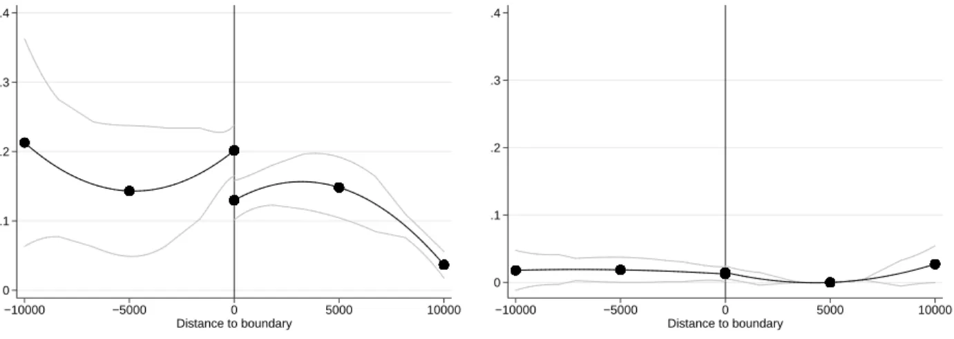
I begin by graphically analyzing the relationship between electoral fraud and cell phone cov-erage using RD plots of the outcome variable. Figures 4.3a and 4.3b plot the avcov-erage share of Category C+ fraud for polling centers falling within 5-kilometer distance bins for the Southeast and Northwest regions, respectively. Solid dots represent the binned averages. Negative values of distance indicate polling centers in non-coverage areas. The solid line trends give the predicted values from a regression of the variable of interest on a second degree polynomial in distance to the boundary. The window of analysis is 15 kilometers on each side of the boundary and I estimate these regressions separately on each side.

Figure 4.3a shows that within a narrow window around the coverage threshold, the average level of fraud drops sharply for centers located on the coverage side. The average share of Cate-gory C+ fraud for centers within 5 kilometers of the boundary is around 7 to 8 percentage points lower on the coverage side. This compares to an average share of around 20 percent observed in centers on the non-coverage side within that same distance window. Further, average fraud lev-els are consistently higher on the non-coverage side and exhibit a declining trend on the coverage

20_{I define the regions based on the International Security Assistance Forces (ISAF) regional commands}

classifi-cation specified in the Measuring Impacts of Stabilization Initiatives (MISTI) dataset (MISTI 2013). ISAF divided Afghanistan into six regional command centers: Central (Kabul), East, North, South, Southwest, and West. I collapse the regions into Southeast (East, Central, South) and Northwest (North, West, and Southwest). Refer to Appendix Figure C.2 for a depiction of the two regions.