Diwei Zheng, Li Yan and Yu Wang
College of Computer Science and Technology, Nanjing University of Aeronautics and Astronautics, Nanjing,China
Spatial Index for Uncertain Time
Series
A search for patterns in uncertain time series is time-expensive in today's large databases using the currently available methods. To accelerate the search process for uncertain time series data, in this paper, we explore a spatial index structure, which uses uncer-tain information stored in minimum bounding rectan-gle and ameliorates the general prune/search process along the path from the root to leaves. To get a better performance, we normalize the uncertain time series using the weighted variance before the prune/hit pro-cess. Meanwhile, we add two goodness measures with respect to the variance to improve the robustness. The extensive experiments show that, compared with the primitive probabilistic similarity search algorithm, the prune/hit process of the spatial index can be more effi-cient and robust using the specific preprocess and vari-ant index operations with just a little loss of accuracy.
ACM CCS (2012) Classification: Mathematics of computing → Probability and statistics → Statistical paradigms → Time series analysis
Information systems → Information retrieval → Re-trieval models and ranking → Similarity measures
Keywords: time series, spatial index, uncertainty, varying distance threshold
1. Introduction
Time series widely exists in various application fields such as GIS [6], stock market [16], as-tronomy [33], [37], medical application [36], etc. With the development of modern tech-nology and applications, the requirements of dealing with time series dramatically increases. There are several examples of processing time series data. In medical application [36],
re-al-time health timestamp data are used to detect patients' health condition. In the stock market [16], time series data are used to predict the val-ues of the index in upcoming days. In GIS [6], a recognition system is proposed for time series data through acoustic emission. More recently, time series are used for modeling coronal mass ejection in [33], [37], which are analyzed by clustering and visualization [34], [35].
With massive time series data available, an ef-ficient process for searching a specific pattern from the database is clearly becoming more and more essential. A lot of effort has been devoted to working with time series and some essential issues have been investigated, such as probabi-listic range queries [13], [19], similarity match for uncertain time series [2], [7], [9], [11], pat-tern detection for uncertain data [18], and so on. Among these issues, one of the common requirements is to efficiently find probabilisti-cally approximate matches from a collection of data items for a given query item.
implicitly or explicitly represented by geome-try metrics including distance, margin and area [24].
Uncertainty extensively happens in the real world and has been studied in [1]–[4], [7], [9], [11], [12], [14], [15], [17], [18]. Instead of storing a single value at each timestamp in the classical time series, each timestamp can be modeled as a range of possible bucket or a variable with noise that is linked with a proba-bility density function (pdf). In contrast to the deterministic time series, similarity queries for the uncertain one is more uncertain due to the underlying noise of data objects. As a result, the returned answers are always probably approxi-mately correct, with probability 1 – δ indicating degrees in which they meet the query.
Traditional time series with a large size is fac-ing an overhead in efficiency, let alone the un-certain time series. For the massive data set consisting of the uncertain time series, match-ing or searchmatch-ing is not simple, since we need to consider a huge number of noisy items taking along some probability information. Taking the probability information into consideration sig-nificantly increases the time cost in similarity metric calculation [3]. In addition, the existing classical time series models cannot properly cooperate with uncertain information. Hence, a lot of effort has been carried out for the uncer-tain time series in several indirect ways, such as transforming the original question into classical deterministic models [19], [31], modifying tra-ditional measurements or proposing new mea-surements [2], [3], [9], [17] and optimization operations [15].
Uncertain data management has been studied in the context of databases and now it resurges anew with the development of modern technol-ogy and applications. Due to the efficient algo-rithm for the ideal data object without noise, it is indispensable to carefully reconstruct the structure to embed uncertain information. We strive to develop faster-searching methods to search a database consisting of a plenty of time series. Although the spatial index (e.g.,
R*-trees) can be used to search approximation
queries, this approach exploits two assump-tions: the first one is that data sequences and query sequences all have the same length; the second one is that the sequences are all
defi-nite. The probabilistic approach to processing similarity queries over uncertain data streams, namely (PROUD) [2] and the novel distance measure DUST [3] are both time-expensive methods since the prune/hit process involves integral calculation over the pdf. The traditional spatial index methods simply ignore the noise behind the item and do not take advantage of variance in each timestamp at all. This causes a heavy accuracy loss in final results.
In this paper, we explore a spatial index struc-ture in connection with the uncertainty entries. Based on the PROUD, we plug and exploit the variance in minimum bounding rectangle (MBR) which is a directory for speeding up search process in the spatial index and refine the general prune/search process along the path from the root to leaves. To keep a better approximation in metric measures defined in a Euclidean distance, we propose a new prepro-cess method with weighted variance for uncer-tain times series. At the same time, we improve the robustness of the index using the variance in each MBR. Our contributions in this paper are summarized as follows:
1. We accommodate uncertain information in the classical spatial index R*-tree and show that the key to the combination is the uncertain monotonic direction of the dis-tance threshold.
2. We investigate how to use the variance of uncertainty information to make less visits to deeper nodes, which will evidently im-prove the index robustness.
3. We propose a heuristic method with the variance taken into consideration to prune the candidates of the time series in which each time stamp has different random vari-ance.
The rest of this paper is organized as follows. In Section 2, we give a brief description of the related work for the uncertain time series. Sec-tion 3 presents the model and the algorithm
PROUD proposed in [2] for the uncertain time
series. We present how to combine uncertain-ties with a classical index to efficiently search and construct a variant spatial index in Section 4. The experiments are presented in Section 5. We finally conclude the paper in Section 6.
and process time-sequenced data. Efficient que-ries contain two vital steps, as shown in Figure 1.
1. Preprocess. In the real world, we are al-ways stuck in a dilemma of balancing ac-curacy and efficiency. This question is a complex overhead when the length of the series is too long to efficiently calculate a metric. Thus, several methods (e.g., Wave-let decomposition [26] and Discrete Fouri-er transform (DFT)) were proposed to ex-tract the features of series and reduce the original dimension to a new space, which has the least loss in retrieving values. In essence, the operation of dimension reduc-tion is to map the points in a space with higher dimension into a lower dimensional space which is spanned by only a few new orthogonal vectors.
2. Index. After the preprocess in which every value of the timestamp is mapped into a new space, each time series can be corre-spondingly regarded as a point in this new space. It is clear that the spatial index can be constructed with those points. Based on some classical index structures such as
R*-tree, X-tree, S-tree and so on, the target
measurement can be directly calculated by coefficients in the index or implicitly ob-tained by retrieval values. Note that most of the existing work is focused on exact data without noise. The assumption with the noise absent is hardly adaptable to the physical environment which always con-tains uncertainties.
2.3. Index for Managing Uncertain Time Series
To rapidly deal with the large sequences with limited computation source, summarization methods for data streams have been
consid-2. Related Work
2.1. Uncertain Time Series and Querying
There has been plenty of work on representing and querying uncertain data. However, only a few parts of them address querying and index-ing uncertain time series data. So far, there are two kinds of the proposed models for uncertain time series. The first one views the timestamp as a bucket used to record the historical values and the second one, called a pdf-based model, regards each timestamp as a variable with a ran-dom error noise. On the basis of the set, the no-tion of uncertain time series was formalized and two novel and essential types of range queries over uncertain time series were proposed in [1]. However, the number of combination choices for the series is exponential and must be re-fined by the boundaries proposed in [1]. In [2],
PROUD, which is based on the Central Limit
Theorem, was presented in the pdf-based model and offered a flexible control through distance or probability thresholds defined by users. The experiments in [2] showed exactly a trade-off between false alarms and false drops controlled by the user-defined distance and probability. In [3], the notion of the measurement for the un-certain time series was generalized, in which, based on several properties, more probabili-ty statistical information (e.g., totally various
pdfs) were accommodated. In each timestamp, the measurement named DUST was quantified by approximately comparing the probabilities using the inequation
(
)
(
1,)
(
(
2,)
)
.P DIST X Y ≤ε >P DIST X Y ≤ε
In [9], [17], the relationship between two se-ries was explored through the correlation sta-tistics. And with a preprocess, the relationship was used to convert the correlation threshold into the distance threshold. Finally, they used the measurement on both pdf-based model and multiset-based model in experiments and showed a flexible result of the measurement.
2.2. Index Method for Classical Time Series
With a large number of time series data avail-able, there have been several efforts to model
Preprocess Index
OriginalData Search
ered. However, for uncertain time series, few proposed indexes can be used for uncertain sta-tistics.
The first effort was regarding uncertain time se-ries as cloaked time sese-ries based on a synopsis model in which each time stamp only knows the mean and deviation of the variance. The pattern match query was redesigned to work togeth-er with this model. Due to the dimensionality curse, a more efficient algorithm was proposed to construct the index with extra statistics such as mean and variance. Based on the framework proposed in [20], a more flexible measurement was offered in [2] by using the cumulative distribution function (cdf), which controls the false/true alarms or false/true drops. Aiming to efficiently prune unqualified series, a Haar
decomposition index was used in [2]. The mea-surement can be directly calculated from the decomposed values in the index. However, it only focuses on the update operation for infinite stream data in a limited memory source. It can get more flexibility but without great efficiency improvement in the prune process.
Note that using the methods like feature ex-traction or decomposition based on different models or different assumptions, index struc-ture should be explicitly or implicitly modified to adapt to the uncertainty information. In this paper, we propose a spatial index which can be generalized to expand the content of MBR
and uses the uncertain parameter to update the structure.
It is clear that the preprocess such as dimension reduction, normalization, etc. can enhance the performance of index. However, as we can see, there is no great progress in the index and the classical index still keeps an original state even when we face a greatly different data object. So far, the study about the preprocess for uncer-tain time series receives a lot of attention while the optimization is ignored. In this paper, we present an optimized spatial index R*-tree for the uncertain time series, as well as a modified preprocess which cooperate with uncertainty information.
3. Preliminaries
In this section, we introduce the model used for uncertain time series as well as the algorithm
PROUD based on the model in [2]. Although
the multi-based model proposed in [1] can be also indexed abruptly, the exponential number of the combination is time-costly and the op-timization method in [1] can only be taken at the level of the leaves. So, we use a continuous model for uncertain time series and develop a variant index based on this model.
3.1. Continuous Model
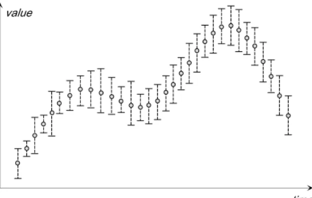
An uncertain time series ˆSu is a time series that may contain uncertainty at each time point. Given a time point j, the value of the uncertain time series at j is denoted by S jˆu
[ ]
and is rep-resented as follows [20][ ]
ˆu uj uj.
S j =d +e
Here duj is the true data value and euj is the
arbi-trary error. An uncertain time series is illustrat-ed in Figure 2.
The above model of uncertain time series re-gards a timestamp as a variance and the pruned framework deals with the probability statistics. A measurement based on the probability func-tion is explored in [2], which transforms the question into a cumulative distribution func-tion (cdf). With a generation notion about the measurement for uncertain time series, a nov-el measurement quantifying the uncertainty is proposed in [3], which will degenerate to the Euclidean distance when the distance is large enough relative to the error.
3.2. PROUD
We define ˆSref as a reference series with un-certainty and ˆSu as one of the items with noise stored in the database. Both kinds of series con-sist of the random variable in each time series. Given the definition of
(
ˆref,ˆu)
(
ˆref[ ]
ˆu[ ]
)
2,i
Dst S S =
∑
S i S i−searching solves the probabilistic problem with user defined distance threshold r and probabili-ty threshold τ∈ (0,1] [2]
(
(
)
)
2 ˆref,ˆu .Pr Dst S S ≤r ≥τ
(1)
PROUD [2] addresses an efficient judge
in-equation which is transformed from the origi-nal question for selecting candidates utilizing the property of cumulative distribution.
According to the Central Limit Theorem, the distance between ˆSref and ˆSu namely
(
ˆref, ˆu)
Dst S S is treated as a joint variable with
a corresponding mean and variance
(
ˆref, ˆu)
(
(
ˆref,ˆu) (
, ˆref, ˆu)
)
.Dst S S N E S S Var S S
(2) Note that the cdf of a normal distribution can be expressed in terms of the well-known error function. Given the mean μ and the deviation σ
of a random variable X with a normal distribu-tion, its cdf can be formalized as follows:
(
)
Ö ,( )
12 1 .2
x
P X x µ σ x erf σ µ
−
≤ = = +
(3) Finally, the cumulative distribution of the vari-able modeled by a pair of time series X and Y
can be defined as:
(
)
(
)
(
) (
)
(
)
(
)
2 ˆ ,ˆ
ˆ , ˆ ˆ , ˆ
1 1 .
2 2 ˆ , ˆ
ref u
ref u ref u
ref u
Pr Dst S S r
Dst S S E S S
erf
Var Dst S S
≤
−
= +
(4)
Since the monotonicity of ϕ increases, the can-didates for the uncertain time series can be eventually transformed into the following in-equation.
(
)
(
(
(
(
)
)
)
)
(
)
2
1
ˆ , ˆ ˆ ,ˆ
ˆ ˆ
2 ,
2 2 1 .
ref u
norm ref u
ref u
r E Dst S S
r S S
Var Dst S S
erf− τ r limit
− =
≥ − = −
(5) Here, r-limit is a normalized threshold for the matching process. The error ratio is defined as the number of incorrect candidates divided by all candidates and the miss ratio is defined as the correct candidates divided by all correct candidates. Experiments in [2] show a flexible trade-off between the error ratio and the miss ratio through the user-defined distance thresh-old and probability threshthresh-old.
4. Index Construction with
Uncertainty
In this section, we propose a novel approach to index the uncertain time series based on
PROUD. Resulting from the uncountable
mea-surement in PROUD, the first step is to give a measurable distance such as Euclidean and keep the same solution space compared to the prim-itive question. Then we find the correlation be-tween the index structure and the measurement, with respect to the two user-defined thresholds. In the experiment, we find the limitation of the index for uncertain time series, especially for the one with the large noise. Hence, it is neces-sary to give a preprocess and optimization op-eration for the matching process.
4.1. Index Construction for Uncertain Time Series
We use a synopsis model with the PROUD
scheme. Although there is a Haar decomposi-tion on the PROUD, the index concentrates on the single stream data prune process and does not make use of the any relationship between two time series. We define ˆSref as a reference
series with uncertainty and ˆSu as a series with YDOXH
WLPH
ered. However, for uncertain time series, few proposed indexes can be used for uncertain sta-tistics.
The first effort was regarding uncertain time se-ries as cloaked time sese-ries based on a synopsis model in which each time stamp only knows the mean and deviation of the variance. The pattern match query was redesigned to work togeth-er with this model. Due to the dimensionality curse, a more efficient algorithm was proposed to construct the index with extra statistics such as mean and variance. Based on the framework proposed in [20], a more flexible measurement was offered in [2] by using the cumulative distribution function (cdf), which controls the false/true alarms or false/true drops. Aiming to efficiently prune unqualified series, a Haar
decomposition index was used in [2]. The mea-surement can be directly calculated from the decomposed values in the index. However, it only focuses on the update operation for infinite stream data in a limited memory source. It can get more flexibility but without great efficiency improvement in the prune process.
Note that using the methods like feature ex-traction or decomposition based on different models or different assumptions, index struc-ture should be explicitly or implicitly modified to adapt to the uncertainty information. In this paper, we propose a spatial index which can be generalized to expand the content of MBR
and uses the uncertain parameter to update the structure.
It is clear that the preprocess such as dimension reduction, normalization, etc. can enhance the performance of index. However, as we can see, there is no great progress in the index and the classical index still keeps an original state even when we face a greatly different data object. So far, the study about the preprocess for uncer-tain time series receives a lot of attention while the optimization is ignored. In this paper, we present an optimized spatial index R*-tree for the uncertain time series, as well as a modified preprocess which cooperate with uncertainty information.
3. Preliminaries
In this section, we introduce the model used for uncertain time series as well as the algorithm
PROUD based on the model in [2]. Although
the multi-based model proposed in [1] can be also indexed abruptly, the exponential number of the combination is time-costly and the op-timization method in [1] can only be taken at the level of the leaves. So, we use a continuous model for uncertain time series and develop a variant index based on this model.
3.1. Continuous Model
An uncertain time series ˆSu is a time series that may contain uncertainty at each time point. Given a time point j, the value of the uncertain time series at j is denoted by S jˆu
[ ]
and is rep-resented as follows [20][ ]
ˆu uj uj.
S j =d +e
Here duj is the true data value and euj is the
arbi-trary error. An uncertain time series is illustrat-ed in Figure 2.
The above model of uncertain time series re-gards a timestamp as a variance and the pruned framework deals with the probability statistics. A measurement based on the probability func-tion is explored in [2], which transforms the question into a cumulative distribution func-tion (cdf). With a generation notion about the measurement for uncertain time series, a nov-el measurement quantifying the uncertainty is proposed in [3], which will degenerate to the Euclidean distance when the distance is large enough relative to the error.
3.2. PROUD
We define ˆSref as a reference series with un-certainty and ˆSu as one of the items with noise stored in the database. Both kinds of series con-sist of the random variable in each time series. Given the definition of
(
ˆref,ˆu)
(
ˆref[ ]
ˆu[ ]
)
2,i
Dst S S =
∑
S i S i−searching solves the probabilistic problem with user defined distance threshold r and probabili-ty threshold τ∈ (0,1] [2]
(
(
)
)
2 ˆref,ˆu .Pr Dst S S ≤r ≥τ
(1)
PROUD [2] addresses an efficient judge
in-equation which is transformed from the origi-nal question for selecting candidates utilizing the property of cumulative distribution.
According to the Central Limit Theorem, the distance between ˆSref and ˆSu namely
(
ˆref, ˆu)
Dst S S is treated as a joint variable with
a corresponding mean and variance
(
ˆref, ˆu)
(
(
ˆref,ˆu) (
, ˆref, ˆu)
)
.Dst S S N E S S Var S S
(2) Note that the cdf of a normal distribution can be expressed in terms of the well-known error function. Given the mean μ and the deviation σ
of a random variable X with a normal distribu-tion, its cdf can be formalized as follows:
(
)
Ö ,( )
12 1 .2
x
P X x µ σ x erf σ µ
−
≤ = = +
(3) Finally, the cumulative distribution of the vari-able modeled by a pair of time series X and Y
can be defined as:
(
)
(
)
(
) (
)
(
)
(
)
2 ˆ ,ˆ
ˆ , ˆ ˆ , ˆ
1 1 .
2 2 ˆ , ˆ
ref u
ref u ref u
ref u
Pr Dst S S r
Dst S S E S S
erf
Var Dst S S
≤
−
= +
(4)
Since the monotonicity of ϕ increases, the can-didates for the uncertain time series can be eventually transformed into the following in-equation.
(
)
(
(
(
(
)
)
)
)
(
)
2
1
ˆ , ˆ ˆ ,ˆ
ˆ ˆ
2 ,
2 2 1 .
ref u
norm ref u
ref u
r E Dst S S
r S S
Var Dst S S
erf− τ r limit
− =
≥ − = −
(5) Here, r-limit is a normalized threshold for the matching process. The error ratio is defined as the number of incorrect candidates divided by all candidates and the miss ratio is defined as the correct candidates divided by all correct candidates. Experiments in [2] show a flexible trade-off between the error ratio and the miss ratio through the user-defined distance thresh-old and probability threshthresh-old.
4. Index Construction with
Uncertainty
In this section, we propose a novel approach to index the uncertain time series based on
PROUD. Resulting from the uncountable
mea-surement in PROUD, the first step is to give a measurable distance such as Euclidean and keep the same solution space compared to the prim-itive question. Then we find the correlation be-tween the index structure and the measurement, with respect to the two user-defined thresholds. In the experiment, we find the limitation of the index for uncertain time series, especially for the one with the large noise. Hence, it is neces-sary to give a preprocess and optimization op-eration for the matching process.
4.1. Index Construction for Uncertain Time Series
We use a synopsis model with the PROUD
scheme. Although there is a Haar decomposi-tion on the PROUD, the index concentrates on the single stream data prune process and does not make use of the any relationship between two time series. We define ˆSref as a reference
series with uncertainty and ˆSu as a series with YDOXH
WLPH
noise stored in the database. Both kinds of se-ries consist of the random variable in each time-stamp. In [2], a pruned algorithm is explored by using the inequation rnorm
(
Sˆref,Sˆu)
≥ −r limitfor the candidates satisfying the following filter inequation:
(
)
(
)
(
) (
)
(
)
(
)
2 ˆ ,ˆˆ , ˆ ˆ , ˆ
1 1 .
2 2 ˆ ,ˆ
ref u
ref u ref u
ref u
Pr Dst S S r
Dst S S E S S
erf
Var Dst S S
≤ − = + (6) To construct the spatial index with Euclidean
distance, we delve further into the algorithm
PROUD to transform this uncountable
mea-surement into a monotonic and consecutive form. In particular, under the assumption of the same distribution of timestamp in a time se-ries for the sake of simplicity, the prune func-tion can be changed as the following equafunc-tion, which is a vital transformation for equal justice of candidates.
(
)
(
)
(
)
(
)
(
)
(
)
(
)
( )
(
)
(
)
( )
(
)
(
)
( )
(
)
2 2 1 2 2 2 1 2 2 2 2 2 1 2 2 2 2 ˆ , ˆˆ , ˆ ˆ ,ˆ
4
0 4
0 2
. . 4 0, 1,
4 , ref u ref u ref u len r i i i len r r i i i r len r i i i r
Pr Dst S S r limit
r E Dst S S
r limit
Var Dst S S
r
limit
r len
b b ac
a
s t b ac a
b r limit
c r le
τ
µ µ
σ σ µ µ
σ σ µ µ σ σ = = = ≤ − ≥ − ⇒ ≥ − ⇒ − + − + − − − + ≤ − + − ⇒ ≤ − ≤ − ≥ = = − + = − +
∑
∑
∑
( )
(
2 r 2)
n σ + σ
(7)
where E Dst S
(
(
ˆref,Sˆu)
)
and Var Dst S(
(
ˆref,Sˆu)
)
are expanded and calculated in [2]. As we can see, the derivation explores the possibility of transforming an uncertain uncountable mea-surement into an exact monotonic form for dy-namic progress. The last inequation turns out that PROUD can be changed as a Euclidean dis-tance for the variance. Also, Wavelet
Summari-zation is proposed in [2] for online stream data
decomposition in a dynamic environment. It is focused on how to retain the vital coefficient in a limited memory source and on efficient summarization by keeping from extracting the coefficients from the index structure. Howev-er, they do not take into consideration the rela-tionship of uncertain information between two random time series. On the contrary, we make full use of the uncertain information in each se-ries by the inequation (7). As we can see, the required operation for the uncertain time series changes as a deterministic requirement for the series that consists of the means. However, the distance thresholds for these series are different from each other. The monotonic property must be shown as follows:
( ) (
)
(
( )
)
( )
2
2 2 2 2
2 2 -r r
VarThd r limit len r r limit
σ σ σ
σ σ = − + + − + (8)
( )
(
)
( )
(
)
(
)
(
( )
)
( )
(
)
(
( )
)
(
)
(
)
(
( )
)
( )
2 2 2 2 2 2 22 2 2 2
2
2 2 2
2 2
2 2 2 2
-2 -- -2 -r r r r r r dVarThd d
r limit len
r limit len r
r limit r limit len r
r limit len r
σ σ
σ σ
σ σ σ σ
σ σ
σ σ σ σ
− + = − + + + − + + − − + + + (9) with a valid user-defined probability thresh-old τ in [0,1], as well as the value of r-limit
in −4 2,4 2. Since the length is always greatly larger than 4 2, which is a very triv-ial condition, the varying distance threshold is
monotonically decreasing along σ when τ ≥ 0.5.
Most of the time, the length of the sequence is larger than the limited r-limit. Then we can as-sume that the coefficient r-limit – len is always a negative. With those sign assumptions, we can judge the monotonic property for σ, which is described in the following theorem.
Theorem 1. The function ( )f x =a x b ax c− +
with a < 0, 4 2− ≤ ≤b 4 2, c ≥ 0, x ≥ 0 is a
negative if b > 0 or x b c a a b> 2 / ( ( − 2)) and a positive if 0≤ ≤x b c a a b2 / ( ( − 2)).
The theorem is simple and here we ignore the concrete detail of its proof, which is present in the appendix. We present a corresponding ex-ample of the varying threshold in Figure 3.
In our actual application, we define a =
r-limit2 – len, b = r-limit and c = r2, x = σ2 +
(σr)2. Therefore, according to Theorem 1, with
the case τ > 0.5, we have r-limit > 0 and the
Var-Threshold is monotonically decreasing with σ2
+ (σr)2. However, if r-limit ≤ 0 namely τ ≤ 0.5,
there are two monotonical directions which are divided by b2c/(a(a – b2)) named critical point.
When the critical point is located in the range
[σmin, σmax] in an MBR, we must check both σmin
and σmax for the minimum threshold and
calcu-late the maximum threshold by critical point using b2c/(a(a – b2)).
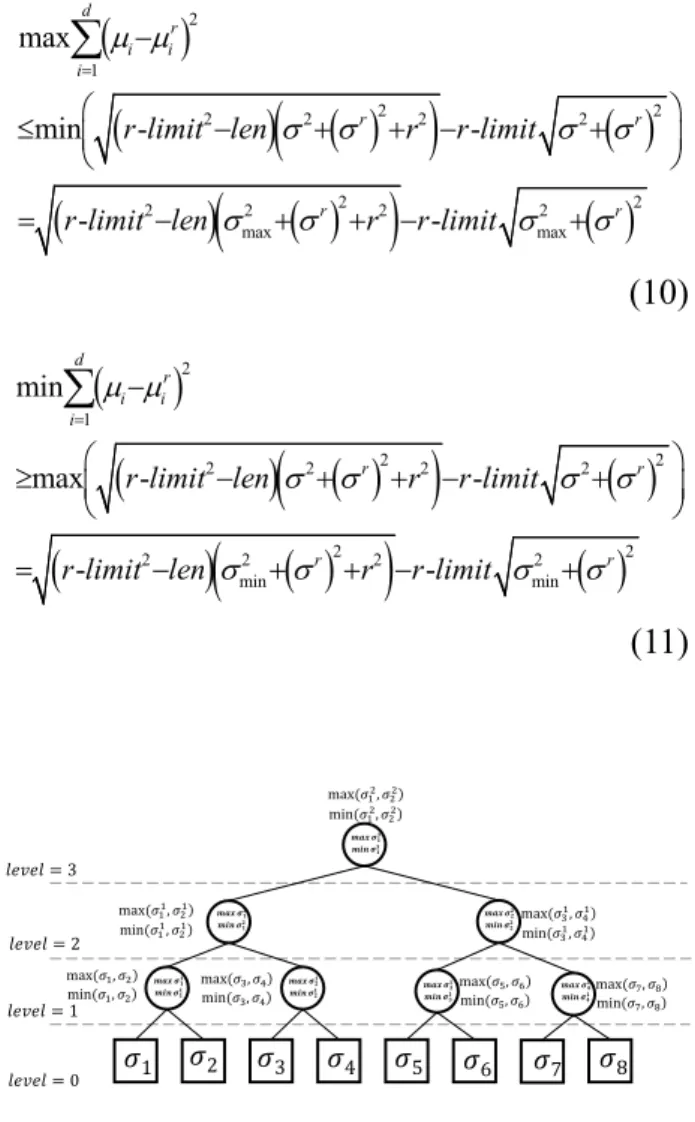
Finally, an MBR in Figure 4 can be judged di-rectly if it satisfies one of the following inequa-tions:
(
)
(
) ( )
(
)
( )
(
)
(
( )
)
( )
2 1 2 22 2 2 2
2 2
2 2 2 2
max max
max
min -
-- -d r i i i r r r r
r limit len r r limit
r limit len r r limit
µ µ
σ σ σ σ
σ σ σ σ
= − ≤ − + + − + = − + + − +
∑
(10)(
)
(
) ( )
(
)
( )
(
)
(
( )
)
( )
2 1 2 22 2 2 2
2 2
2 2 2 2
min min
min
max -
-- -d r i i i r r r r
r limit len r r limit
r limit len r r limit
µ µ
σ σ σ σ
σ σ σ σ
= − ≥ − + + − + = − + + − +
∑
(11)All leaf entries included in an index node sat-isfying the first inequation must be the candi-dates because no VarThd in all entries included in the MBR could be larger than their parent nodes. Therefore, the distance of leaf nodes to
μref covered by children entries must satisfy the
first inequation, whereas those satisfying the second inequation must be pruned. Also, both extreme distances must be in the corners of the
MBR, which means the complexity of finding max and min distances is O(N), where N is the dimension of the point.
0 10 20 30 40 50 60 VarThd ı2
Figure 3. Varying threshold.
ሺߪଵଶǡ ߪଶଶሻ
ሺߪଵଶǡ ߪଶଶሻ
ࢇ࢞Ԝ࣌
Ԝ࣌
݈݁ݒ݈݁ ൌ ͵
݈݁ݒ݈݁ ൌ ʹ
݈݁ݒ݈݁ ൌ ͳ
݈݁ݒ݈݁ ൌ Ͳ
ሺߪଵଵǡ ߪଶଵሻ
ሺߪଵଵǡ ߪଶଵሻ
ࢇ࢞Ԝ࣌
Ԝ࣌
ሺߪଷଵǡ ߪସଵሻ
ሺߪଷଵǡ ߪସଵሻ
ࢇ࢞Ԝ࣌
Ԝ࣌
ሺߪଵǡ ߪଶሻ
ሺߪଵǡ ߪଶሻ
ࢇ࢞Ԝ࣌
Ԝ࣌ ሺߪଷǡ ߪସሻ
ሺߪଷǡ ߪସሻ
ሺߪହǡ ߪሻ
ሺߪହǡ ߪሻ
ࢇ࢞Ԝ࣌
Ԝ࣌ ሺߪǡ ߪ଼ሻ
ሺߪǡ ߪ଼ሻ
ࢇ࢞Ԝ࣌
Ԝ࣌
ߪͳ ߪʹ ߪ͵ ߪͶ ߪͷ ߪ ߪ ߪͺ
ࢇ࢞Ԝ࣌
Ԝ࣌
Figure 4. MBR with σ.
r-limit = 2, len = 40, σr = 1, r = 50
0 10 20 30 40 50 60 VarThd ı2
noise stored in the database. Both kinds of se-ries consist of the random variable in each time-stamp. In [2], a pruned algorithm is explored by using the inequation rnorm
(
Sˆref,Sˆu)
≥ −r limitfor the candidates satisfying the following filter inequation:
(
)
(
)
(
) (
)
(
)
(
)
2 ˆ ,ˆˆ , ˆ ˆ , ˆ
1 1 .
2 2 ˆ ,ˆ
ref u
ref u ref u
ref u
Pr Dst S S r
Dst S S E S S
erf
Var Dst S S
≤ − = + (6) To construct the spatial index with Euclidean
distance, we delve further into the algorithm
PROUD to transform this uncountable
mea-surement into a monotonic and consecutive form. In particular, under the assumption of the same distribution of timestamp in a time se-ries for the sake of simplicity, the prune func-tion can be changed as the following equafunc-tion, which is a vital transformation for equal justice of candidates.
(
)
(
)
(
)
(
)
(
)
(
)
(
)
( )
(
)
(
)
( )
(
)
(
)
( )
(
)
2 2 1 2 2 2 1 2 2 2 2 2 1 2 2 2 2 ˆ , ˆˆ , ˆ ˆ ,ˆ
4
0 4
0 2
. . 4 0, 1,
4 , ref u ref u ref u len r i i i len r r i i i r len r i i i r
Pr Dst S S r limit
r E Dst S S
r limit
Var Dst S S
r
limit
r len
b b ac
a
s t b ac a
b r limit
c r le
τ
µ µ
σ σ µ µ
σ σ µ µ σ σ = = = ≤ − ≥ − ⇒ ≥ − ⇒ − + − + − − − + ≤ − + − ⇒ ≤ − ≤ − ≥ = = − + = − +
∑
∑
∑
( )
(
2 r 2)
n σ + σ
(7)
where E Dst S
(
(
ˆref,Sˆu)
)
and Var Dst S(
(
ˆref,Sˆu)
)
are expanded and calculated in [2]. As we can see, the derivation explores the possibility of transforming an uncertain uncountable mea-surement into an exact monotonic form for dy-namic progress. The last inequation turns out that PROUD can be changed as a Euclidean dis-tance for the variance. Also, Wavelet
Summari-zation is proposed in [2] for online stream data
decomposition in a dynamic environment. It is focused on how to retain the vital coefficient in a limited memory source and on efficient summarization by keeping from extracting the coefficients from the index structure. Howev-er, they do not take into consideration the rela-tionship of uncertain information between two random time series. On the contrary, we make full use of the uncertain information in each se-ries by the inequation (7). As we can see, the required operation for the uncertain time series changes as a deterministic requirement for the series that consists of the means. However, the distance thresholds for these series are different from each other. The monotonic property must be shown as follows:
( ) (
)
(
( )
)
( )
2
2 2 2 2
2 2 -r r
VarThd r limit len r r limit
σ σ σ
σ σ = − + + − + (8)
( )
(
)
( )
(
)
(
)
(
( )
)
( )
(
)
(
( )
)
(
)
(
)
(
( )
)
( )
2 2 2 2 2 2 22 2 2 2
2
2 2 2
2 2
2 2 2 2
-2 -- -2 -r r r r r r dVarThd d
r limit len
r limit len r
r limit r limit len r
r limit len r
σ σ
σ σ
σ σ σ σ
σ σ
σ σ σ σ
− + = − + + + − + + − − + + + (9) with a valid user-defined probability thresh-old τ in [0,1], as well as the value of r-limit
in −4 2,4 2. Since the length is always greatly larger than 4 2, which is a very triv-ial condition, the varying distance threshold is
monotonically decreasing along σ when τ ≥ 0.5.
Most of the time, the length of the sequence is larger than the limited r-limit. Then we can as-sume that the coefficient r-limit – len is always a negative. With those sign assumptions, we can judge the monotonic property for σ, which is described in the following theorem.
Theorem 1. The function ( )f x =a x b ax c− +
with a < 0, 4 2− ≤ ≤b 4 2, c ≥ 0, x ≥ 0 is a
negative if b > 0 or x b c a a b> 2 / ( ( − 2)) and a positive if 0≤ ≤x b c a a b2 / ( ( − 2)).
The theorem is simple and here we ignore the concrete detail of its proof, which is present in the appendix. We present a corresponding ex-ample of the varying threshold in Figure 3.
In our actual application, we define a =
r-limit2 – len, b = r-limit and c = r2, x = σ2 +
(σr)2. Therefore, according to Theorem 1, with
the case τ > 0.5, we have r-limit > 0 and the
Var-Threshold is monotonically decreasing with σ2
+ (σr)2. However, if r-limit ≤ 0 namely τ ≤ 0.5,
there are two monotonical directions which are divided by b2c/(a(a – b2)) named critical point.
When the critical point is located in the range
[σmin, σmax] in an MBR, we must check both σmin
and σmax for the minimum threshold and
calcu-late the maximum threshold by critical point using b2c/(a(a – b2)).
Finally, an MBR in Figure 4 can be judged di-rectly if it satisfies one of the following inequa-tions:
(
)
(
) ( )
(
)
( )
(
)
(
( )
)
( )
2 1 2 22 2 2 2
2 2
2 2 2 2
max max
max
min -
-- -d r i i i r r r r
r limit len r r limit
r limit len r r limit
µ µ
σ σ σ σ
σ σ σ σ
= − ≤ − + + − + = − + + − +
∑
(10)(
)
(
) ( )
(
)
( )
(
)
(
( )
)
( )
2 1 2 22 2 2 2
2 2
2 2 2 2
min min
min
max -
-- -d r i i i r r r r
r limit len r r limit
r limit len r r limit
µ µ
σ σ σ σ
σ σ σ σ
= − ≥ − + + − + = − + + − +
∑
(11)All leaf entries included in an index node sat-isfying the first inequation must be the candi-dates because no VarThd in all entries included in the MBR could be larger than their parent nodes. Therefore, the distance of leaf nodes to
μref covered by children entries must satisfy the
first inequation, whereas those satisfying the second inequation must be pruned. Also, both extreme distances must be in the corners of the
MBR, which means the complexity of finding max and min distances is O(N), where N is the dimension of the point.
0 10 20 30 40 50 60 VarThd ı2
Figure 3. Varying threshold.
ሺߪଵଶǡ ߪଶଶሻ
ሺߪଵଶǡ ߪଶଶሻ
ࢇ࢞Ԝ࣌
Ԝ࣌
݈݁ݒ݈݁ ൌ ͵
݈݁ݒ݈݁ ൌ ʹ
݈݁ݒ݈݁ ൌ ͳ
݈݁ݒ݈݁ ൌ Ͳ
ሺߪଵଵǡ ߪଶଵሻ
ሺߪଵଵǡ ߪଶଵሻ
ࢇ࢞Ԝ࣌
Ԝ࣌
ሺߪଷଵǡ ߪସଵሻ
ሺߪଷଵǡ ߪସଵሻ
ࢇ࢞Ԝ࣌
Ԝ࣌
ሺߪଵǡ ߪଶሻ
ሺߪଵǡ ߪଶሻ
ࢇ࢞Ԝ࣌
Ԝ࣌ ሺߪଷǡ ߪସሻ
ሺߪଷǡ ߪସሻ
ሺߪହǡ ߪሻ
ሺߪହǡ ߪሻ
ࢇ࢞Ԝ࣌
Ԝ࣌ ሺߪǡ ߪ଼ሻ
ሺߪǡ ߪ଼ሻ
ࢇ࢞Ԝ࣌
Ԝ࣌
ߪͳ ߪʹ ߪ͵ ߪͶ ߪͷ ߪ ߪ ߪͺ
ࢇ࢞Ԝ࣌
Ԝ࣌
Figure 4. MBR with σ.
r-limit = 2, len = 40, σr = 1, r = 50
0 10 20 30 40 50 60 VarThd ı2
4.2. Search Strategy
In a recurrence processing that starts from the root of the index, we check all its children and determine if they satisfy one of the above in-equations. It is shown that the time complexity of visiting all nodes in the index is O(1) under the best condition and nearly O(alogb n ) under the
worst condition. If the height of the index is 1, the searching is degenerated into an ordered searching with the worst time complexity of
O(n). Compared with the time for calculating the measurement for two uncertain time series (especially in high dimensions), the visiting time takes up a few parts, meaning that in a global view, the index performance taking ad-vantages outweighs taking disadad-vantages most of the time.
We summarize the searching in Algorithm 2. Given a target series ˆSref and a root R of the
R*-tree index, the time series which are
prepro-cessed in advance, a distance threshold r, and a probability threshold τ, Algorithm 2 outputs a set of all candidates in which the probabili-ties that the distances of these candidates to the target reference series exceed r, is less than τ. First, we start with searching for a path from the root of the index and then compare each pair σmin, σmax in MBRs included in the node.
We check whether the inequation (10) or (11) is satisfied. If the inequation (10) is satisfied, we can directly get the leaves covered by this node. If the inequation (11) is satisfied, we just stop the deeper search along the path from this node. Otherwise, we have a deeper visit in the lower level.
4.3. Random Variance
Given the uncertain time series with the same variance, we construct the leaf entries includ-ing the same minimum and maximum σ valued variance at each timestamp. We can see that the forms of σ boundaries in each MBR are similar to each other. It means that we can heuristically treat the leaf entry as a point that includes the min and max σ in a time series. The following inequation (12) shows the correctness of this heuristic method but it may not be efficient be-cause sometimes the approximation is sensitive to the large amount of noise.
With the max σ, this normalized distance will be minimum. If this minimum distance is larger than the maximum threshold, it satisfies (10), which means that the judge function in the leaf entry is the same as in the internal node of the index. Therefore, we can treat the leaf entry with random σ as internal node hit/pruned by (10)/(11).
( )
(
)
(
)
( )
(
)
(
)
( )
(
)
(
)
( )
(
)
(
)
( )
(
)
(
)
( )
(
)
(
)
2 2 2 2 max max 1 2 2 2 max max 1 2 2 2 2 1 1 2 2 2 1 2 2 2 2 min min 1 2 2 2 min min 1 4 4 4 len r r i i i len r r i i ilen r len r
i i i i
i i
len r r
i i i i
i len r r i i i len r r i i i r len r r len
σ σ µ µ
σ σ µ µ
σ σ µ µ
σ σ µ µ
σ σ µ µ
σ σ µ µ
= = = = = = = − + × + − + − − + + − ≤ + − − + × + − ≤ + −
∑
∑
∑
∑
∑
∑
∑
(12)4.4. Optimization for Random Variance
The result of experiments with random variance time series has shown that the time cost of pro-cessing is close to the one shown by PROUD
for the approximation of the variance. Since
σ has a large variance, the index will hardly
meet the filter equations and always search in leaf entries. For a closer approximation, sever-al preprocesses can be considered. The prepro-cess such as Discrete Fourier transform (DFT) or Moving Average (MA) dimension reduction operation is carried out. Different preprocess-es focus on different targets. DFT focuses on selecting high frequencies and is inefficient for white noise. It merely carries out the dimension reduction by centralizing the energy on several dimensions with high frequency. The MA makes use of the relation of adjacent timestamps for a better approximation for noisy series with prob-abilistic information.
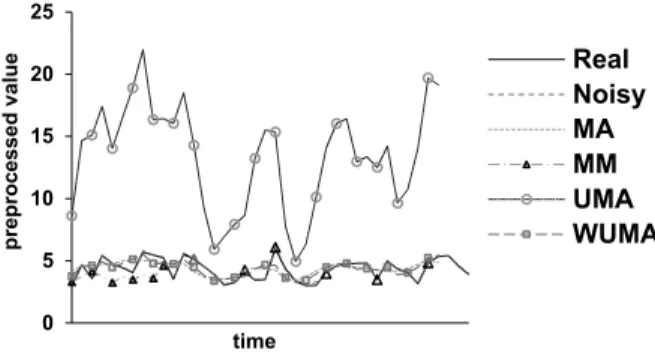
In this paper, we apply a soft preprocess based on MA like [15]. In [15], an Uncertain Moving Average (UMA) is presented to accommodate σ
in a traditional preprocess. There are two kinds of MA for uncertain time series in [15]. The first one is to simply use mathematic average and the second one is based on the exponential func-tion. Both of them are weighted the values by σ
at each timestamp. This means that it is useful for uncertain time series with random σ and the values with larger σ offer less contribution to the final average. For the sake of simplicity, it is assumed that the whole series has the same σ
for presenting the Euclidean distance between
UMA values by classical MA values.
Since
1 , 1
2 1
i w
UMA k
i
k i w k
x
x w + σ i m
= −
= ≤ ≤
+
∑
(13)with a window width w and variance σk
cor-responding to k-th timestamp influences the values sensitively by σk and may change
exces-sively the primitive xk, here we present a new
preprocess named weighted variance uncertain moving average, based on [15].
2 1 , 1 1 i w WUMA k
i i w k
k i w
j j i w
x σ x i m
σ + + = − = − =
∑
≤ ≤∑
(14)It shows that with a larger σ, the values con-tribute less reliable distances to the real original distance. A larger distance with a smaller σ tells us that this stamp is greatly possible to have large real distance and hence greatly contrib-ute to the real distance which will be essential when comparing it with an original threshold. Meanwhile, it keeps a light scale on the primi-tive value.
Suppose that the time series has the same vari-ance in each timestamp, then we have
(
)
1
2 1
i w
WUMA UMA
i k i
k i w
x x x
w σ
+
= −
= =
+
∑
(15)It explores the relationship between xiWUMA
and xiUMA. Compared with UMA, there will
be no difference in performance with a series consisting of the same variance in each time-stamp. Moreover, we normalized the xi with the
weighted σ which will not dramatically affect measurement and hence keep a closer approxi-mation about the sum of all primitive measure-ments. The mean and variance for the normal-ized timestamp are shown in Figure 5.
(
)
(
)
2 31 , 1
1
1 1 , 1
1
i w
WUMA k
i i w
k i w k j
j i w
i w WUMA
i i w
k i w k j
j i w
w
E x i m
Var x i m
σ σ σ σ + + = − = − + + = − = − = ≤ ≤ = ≤ ≤
∑
∑
∑
∑
(16)Algorithm 1. GetCoveredLeaves.
Input: root N of sub tree
Output:LEqueue
1. initialize: Create queue; N ⇒ queue
2. whilequeue is not emptydo
3. cN ⇐ queue
4. fori = 1, ..., cN.childNumdo
5. ifcN.level = 0 then
6. cN.Child[i] ⇒ LEqueue
7. else
8. cN.Child[i] ⇒ queue
9. end if
10. end for
11. end while
push
pop
push
push
Algorithm 2. Search.
Input: root R of R*-tree, ˆ
ref
S target uncertain time series, r distance treshold, τ probability treshold
Output:candidates
1. initialize:
2. Create queue
3. R ⇒ queue
4. r-limit ← 2erf–1(2τ – 1)
5. judge the monotonical property 6. whilequeue is not emptydo
7. cN ⇐ queue
8. fori = 1, ..., cN.childNumdo
9. calculate minimum/maximum tresholds 10. if minimum distance > maximum treshold then
11. //pruned
12. else if maximum distance < minimum treshold then
13. GetCoveredLeaves ⇒ candidates
14. else
15. cN.child[i] ⇒ queue
16. end if
17. end for
18. end while pop push
push


![Figure 9. Preprocess with synthetic data.(b) dratio ∈ [0.1,2.0] 00,20,40,60,811,2 0,1 0,2 0,3 0,4 0,5 0,6 0,7 0,8 0,9err/miss ratioPROUD-ERRIJPROUD-MISSINDEX-ERRINDEX-MISS](https://thumb-us.123doks.com/thumbv2/123dok_us/8037539.2128293/13.1785.966.1537.1830.2210/figure-preprocess-synthetic-dratio-ratioproud-errijproud-missindex-errindex.webp)

