Background-Foreground Segmentation
Based on Dominant Motion Estimation
and Static Segmentation
Yu Huang, Dietrich Paulus, Heinrich Niemann
Chair for Pattern Recognition, Dept. of Computer Science University of Erlangen-N¨urnberg, Erlangen, Germany
This paper addresses the problem of image segmentation using motion and luminance information. We use the dominant motion model to calculate both the background and foreground motion in a robust estimation framework and then combine it with the result of static segmentation using the watershed algorithm to segment the foreground from the background. In this paper, the previous pixel-based(or over a small neighborhood)motion measure is
replaced by the patch-based motion measure in motion segmentation. Experimental results are given to show the efficiency of our method.
Keywords: dominant motion, robust estimation, static segmentation, watershed
1. Introduction
The segmentation of image sequences into re-gions or ‘objects’ has received a large attention in recent years. Applications like object track-ing, video coding and structure from motion can benefit from a meaningful segmentation. But it is by now not solved being a chicken-and-egg problem.
The methods of motion segmentation can be grouped into two broad classes(Sawhney, 1996).
One class solves the problem by letting mul-tiple models simultaneously compete for the description of the individual motion measure-ments (Wang, 1994), and the other excavates
the multiple models sequentially by solving for a dominant model(Irani, 1994). For the former
method, difficulties occur at determination of the number of models or uncertainty of mixture models. The latter may confront puzzles in the case of absence of dominant motion, and it yet lacks competition amongst the motion models.
In this paper, we discuss the dominant motion-based method used for background and fore-ground segmentation. In Sect. 2, we present related works and background. In Sect. 3, the dominant motion estimation method described in(Black, 1996)is outlined, and its combination
with static segmentation using the watershed algorithm is presented. Finally experimental results are reported in Sect. 4 and concluding remarks are given in Sect. 5.
2. Background
The dominant motion model-based method used for segmention, compared to the multiple model competition method, is more efficient because it does not need to consider how many objects occur in the scene and looks simpler from its al-gorithmic form. It is valid for some application fields, for example, background/foreground
seg-mentation.
In the use of dominant motion model, one of the key steps is determination of the dominant object. It is a region or object corresponding to the dominant motion. (Black, 1996)put
for-ward a dominant motion estimation method in a simulated annealing framework, but it can-not give a clean region segmentation since the motion measure of each pixel is individually computed only. (Irani, 1994)also use the
3. Patch-based dominant motion segmentation
In this paper we combine the static segmentation with the dominant motion model. Here over-segmentation is needed in the process of static segmentation in order to make pixels in each subregion having the similar motion. There are some current methods available for this task, for example, the watershed algorithm, the pixel-based region growing and the quadtree split-merge method etc. In this paper, we choose the watershed algorithm. Based on the static segmentation result, we replace the pixel-based motion measure with the proposed patch or region-based motion measure to make a clear segmentation of the dominant motion region.
3.1. The SOR method for dominant motion estimation
Before we present our approach, the Simulta-neous-Over-Relaxation(SOR) method(Black,
1996) for dominant motion estimation is
de-scribed simply. First, the interframe motion is defined as
f(x t+1)= f(x;u(x;a) t) (1)
where f(x t)is the brightness function in time
instantt,x = (x y) is coordinate of the image
pixel, and u(x;a)is the motion vector. We
as-sume the affine flow model(6 parameters) for
the dominant object
u(x;a)=
u(x y)
v(x y)
=
a0+a1x+a2y
a3+a4x+a5y
(2)
where a = (a0 a1 a2 a3 a4 a5)
T are the
pa-rameters of the affine model. This model is valid when the depth variance is small enough com-pared with the depth from the camera. Domi-nant motion estimation is formulated as the fol-lowing robust M-estimator,
min u v ED=
X
(x y)2R
ρ(ufx+v fy+ ft σ) (3)
here theρ – function is chosen as the Geman-McClure function(Black, 1996),
ρ(x σ)=
x2 x2
+σ
2 (4)
withσ as the scale parameter, and fx, fy, ft as partial derivatives of brightness function with respect tox,yandt. The SOR iteration update equations are
a(n+1)
i =a
(n)
i ;ω
@ED
Tai@ai
(5)
withω = 1:995(0< ω <2),Tai as the upper
bound of the second-order partial derivatives, i. e.
Tai @ 2E D @a 2 i
: (6)
The algorithm begins by constructing the Gaus-sian pyramid (we make three levels). At the
coarse level motion is initially set to zero. The number of iterations is chosen as 10. When the estimated parameters are interpolated into the next level, these parameters are used to warp the first image to the second one. In the cur-rent level only the change in the paramenters is estimated in the iterative update scheme. The SOR method lowers the scale parameter
σ according to the formula σn+1
= 0:95σn.
The effect is similar to the simulated anneal-ing method. We set initially σ as 25p
3 and finallyσ (its lower bound)as 15
p
3. Once the dominant motion is estimated the outlying mea-surements are determined by checking the value
fxu
+ fyv+ ft
τ, here τ = σ= p
3. These outlier pixels can be used to determine the next dominant motion parameters.
3.2. Watershed technique of static segmentation
The watershed technique is one of the classics in the field of topography. It regards the gradi-ent magnitude image as a landscape where the brightness values correspond to the elevation. Areas where a rain drop would drain to the same minimum are denoted as catchment basins, and the lines separating adjacent catchment basins are called dividing lines or watersheds.
We obtain the watersheds of the gradient image applying the method in (Vincent, 1991)
filling all the catchment basins, starting from the basin that is associated to the global min-imum. While two catchment basins tend to merge, a dam is built. The process results in partitioning of the image in many catchment basins, of which the borders define the water-sheds. A severe drawback to the computation of watershed images is oversegmentation. Here, though, we need oversegmentation in this proce-dure, but too small partitioned subregions will reduce the accuracy of the following motion labeling process, especially on those poor tex-tured regions. (Vincent, 1991)suggests
modi-fying the gradient function so that the resulting catchment basins correspond only to the desired objects. They put forward two types of methods to realize it, one is region growing, another is utilization of some knowledges on the images studied. Here we use: 1. Prefiltering (mean
value filtering in the 33 neighborhoods) to
allevaite the random noise; 2. After finding the watersheds, the adjacent catchment basins
(4-neighborhoods searching) are further
itera-tively merged (normally the number of
itera-tions is 10)based on thresholding the difference
between two adjacent subregions’ mean values.
3.3. Motion measure
We use the static segmentation to get small re-gions and then determine each region’s motion
measure from MAE(Mean Absolute Error) of
difference between the warped image and the origin image, i. e.
Mi j = X
x2Ri
f
(x t+1);f
Wj
(x t)
=Ci (7)
where fWj
(x t) is the warped image of f(x t)
using thejth dominant motion parameters,Ciis the pixel number in the subregionRi. If we only consider the two dominant motion models in the scene, like the background and foreground seg-mentation, we set j as 2, as for i = 1 2 :::N (Nis the number of regions after static
segmen-tation).
We make the segmentation of the second frame because the motion measure is calculated from its difference with the warped frame. Here we consider two motion models, so directly com-paring the results of (7)and choosing the
mo-tion label j corresponding to the minimal one. Then, we can segment the foreground from
background. If the background is static, i. e. the camera is not moving, we can realize the moving detection too.
4. Results of experiments
We realize the method in C on a SGI work-station. We did experiments with different im-age sequences, mainly considering whether the camera was moving or not. The segmentation from two consecutive images required about 35 seconds, half of time is for static segmentation.
4.1. Static camera
First we give results from two consecutive im-ages in a gait sequence, shown in Fig. 1(a)and
(b). The camera is static, and the person in
the corridor just begins to walk. Image size is 384x256. Fig. 1(c) and (d) shows the
water-shed segmentation results(with the overlapped
region boundaries)before and after merging
ad-jecent regions. Fig. 1(e)and(f) give the
fore-ground segmentation results with the method in
(Black, 1996)and our proposed method on the
same input images respectively. Although in Fig. 1(e) it locates the foreground but cannot
output a clear region. In Fig. 1(f), there exists
some errors in the upper left and right corners of images, they are caused by the calculation error of the motion measure in those subregions warped out of the image. The estimated affine motion parameters are in table 1.
4.2. Moving camera and moving objects
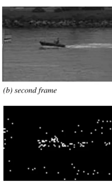
Then the results from two consecutive frames of the standard MPEG ‘Coast Guard’ image se-quence in Fig. 2(a) and (b) are given too, in
which a small boat is moving while the camera is panning. Image size is 352x240. The fig-ures’ location arrangement of Fig. 2 is the same as Fig. 1. From Fig. 2(e) we can find that the
result under natural outdoors scenes using the method in(Black, 1996) can not group
a1] a2] a3] a4] a5]
Foreground 5:176360 0:013673 0:025182 2:629096 0:012113 0:001330
Background 0:197737 ;0:000941 0:000573 0:010358 ;0:000561 0:001848
Table 1.Affine parameters in “gait” images.
(a)first frame (b) second frame (c) watershed segmentation before merging
(d) watershed segmentation after merging (e) dominant (white) pixels (f) dominant motion segmentation
Fig. 1.Gait sequence.
a0] a1] a2] a3] a4] a5]
Foreground ;0:513183 0:002020 ;0:007339 ;0:124831 ;0:003332 0:019044
Background 0:907186 ;0:001687 ;0:004894 0:066219 ;0:000159 0:000222
Table 2.Affine parameters in “Coast guard” images.
(a)first frame (b) second frame (c) watershed segmentation before merging
(d) watershed segmentation after merging (e) dominant (white) pixels (f) dominant motion segmentation
5. Conclusion
We report a motion segmentation method, which combined the static segmentation using the wa-tershed algorithm and the dominant motion mo-del. We replace the pixel-based motion measure with the patch-based motion measure. From given experiment results, we show the method efficiency. In future, we will consider the tem-poral coherence or motion prediction in the motion segmentation from the entire sequence. Meanwhile, we will test its validity in the tasks of posture or gesture recognition.
Acknowledgement
This research is partially supported by Alexan-der von Humboldt foundation.
References
1] BLACKM. J.(1996), The robust estimation of
mul-tiple motions: parametric and piecewise-smooth flow fields,CV & IP, 63(1): 75–104.
2] IRANIM.(1994), Computing occluding and
trans-parent motions, Int. J. Computer Vision, 12(1):
5–16.
3] SAWHNEYH. (1996), Compact representations of
videos through dominant and multiple motion esti-mation,IEEE T-PAMI, 18(8): 814–830.
4] VINCENTL.(1991), Watersheds in digital spaces: a
efficient algorithm based on immersion simulations,
IEEE T-PAMI, 13(6): 583–589.
5] WANGJ.(1994), Representing moving images with
layers,IEEE T-IP, 3(5): 625–638.
Received:October, 2000
Accepted:November, 2000
Contact address:
Yu Huang Dietrich Paulus Heinrich Niemann Chair for Pattern Recognition Dept. of Computer Science University of Erlangen-N¨urnberg 91058, Erlangen, Germany e-mail:[email protected]
DR. YUHUANGwas born in the PR China. He got his B.S. Degree in 1990 at the Dept. of Information & Control Engineering, Xi’an Jiaotong University, Xi’an city, PR China, M.S. degree in 1993 at the Depart-ment of Electrical Engineering, Xidian University, Xian city, PR China, and PhD degree in engineering in 1997 at the Institute of Information Science, Northern Jiaotong University, Beijing, PR China. From April 1997 to April 1999, he was assistant professor and postdoctoral fellow at the Dept. of Computer Science & Technology, Tsinghua Univer-sity, Beijing, PR China. In Sept. 1999 he entered Chair for Pattern Recognition, University of Erlangen-N¨urnberg, Erlangen, Germany, as a research fellow of Prof. H. Niemann, supported by Alexander von Humboldt Foundation. His interests include motion-based segmenta-tion, video indexing, vision-based HCI and Augmented reality.
DR.-ING. DIETRICH PAULUS received his Bachelor Degree in com-puter science from the University of Western Ontario, London, Canada
(1983). He graduated(1987)and received his PhD Degree(1991)and
Habilitation(2000)at Universit¨at Erlangen–N¨urnberg, Germany. He
is presently a senior reseacher(Akademischer Oberrat)in the field of
image pattern recognition and is head of the vision group. He teaches courses in computer vision and applied programming for image pro-cessing. He has written and edited several books and proceedings, in particular on pattern recognition and image processing in C++.
HEINRICHNIEMANNreceived the B.Sc. degree in electrical engineering and the PhD degree from Technical University Hannover in 1966 and 1969, respectively. During 1966/67 he was a graduate student at the
University of Illinois, Urbana. From 1967 to 1972 he was with Fraun-hofer Institut f¨ur Informationsverarbeitung in Technik und Biologie, Karlsruhe, working in the field of pattern recognition and biological cybernetics. During 1973 – 1975 he was teaching at Fachhochschule Giessen in the department of Electrical Engineering. Since 1975 he has been Professor of Computer Science at the University of ErlangenN¨urn-berg, since 1988 he is also head of the research group ‘Knowledge Processing’ at the Bavarian Research Institute for Knowledge Based Systems(FORWISS)where he also was on the board of directors for
six years. During 1979 – 1981 he was dean of the Engineering Faculty of the University.