Knowledge vs. Simulation for Bidding in Tarok
Domen Marinˇciˇc, Matjaž Gams, Mitja Luštrek Department of Intelligent Systems
Jožef Stefan Institute
Jamova 39, SI-1000 Ljubljana, Slovenia
[email protected], [email protected], [email protected]
Keywords:computer games, Bayesian networks, simulation, tarok
Received:
Two approaches for bidding in games are presented: knowledge-based approach and simulation-based approach. A general knowledge-based decision model for bidding in games with its strategy encoded in a Bayesian network was designed. A program for playing four-player tarok was implemented incorporating a specialised instance of the decision model and a simulation module for bidding. Both approaches were compared. The knowledge-based decision model was further compared to human experts, showing that it performs on par with them.
Povzetek: V ˇclanku predstavljamo in primerjamo dva pristopa k reševanju problemov licitiranja v igrah: pristop s predznanjem in pristop s simulacijo.
1 Introduction
Bidding is a part of various card games, for example bridge, poker, tarok and whist. Before the actual card play, players offer to play more and more difficult types of games with the one making the most ambitious offer choosing the type that will be played. Bidding involves exchange of informa-tion between partners (e.g. in bridge) or not (e.g. in tarok or poker). The winner of bidding is the one who actually scores in the game. Since bidding requires the prediction of the final outcome of each type of a game, it is in a way more difficult than card play itself.
In this paper we present and compare two approaches to bidding in tarok [9]: knowledge based-approach and simulation-based approach. For the purpose of compari-son and evaluation we developed the Tarok7 program [10] for four-player tarok. The program uses both (i) an imple-mentation of a decision model based on Bayesian networks and (ii) simulation for bidding. We also examined the pro-gram’s performance under different bidding strategies, and compared it with human experts.
The paper is organized as follows. Rules of bidding in general and in four-player tarok and the most common ap-proaches to bidding in computer games are presented in Section 2. An overview of related work is given in Sec-tion 3. Complexity of different games with bidding is dis-cussed in Section 4. The decision model is described in Section 5. Section 6 presents bidding with simulation as it is performed by Tarok7 program. Section 7 describes the comparison of the two approaches and evaluation of the de-cision model compared to human experts. A conclusion is presented in Section 8.
2 Bidding in Games
In bidding, players bid in a sequence divided into rounds. In one round each player makes one bid. Each bid must be higher than the previous one. Bidding is finished when all players but one pass i.e. do not continue with higher bids. The remaining player is called the declarer. With each type of bid a particular type of game is associated: the higher the bid, the greater the difficulty and the score of the game. The game that corresponds to the last bid of the declarer is played after bidding. These rules hold for most card games such as bridge or tarok. From the strategic point of view, a player has to determine the most difficult type of game which he expects to be able to win according to his strength.
Infour-playertarok, one of the most common games in central Europe, a declarer can play against the other three players teamed together, or choose one partner, depending on his last bid. Teams of players are formed after bidding, which means that players do not know their partners at bid-ding time. Bids influence formation of teams, and set the type of game to be played after bidding. Each type of game has a score bonus which is positive when the declarer wins and negative when he loses. There are 13 types of bids in four-player tarok. We describe 7 of them; others are played rarely. Bonuses are written in parentheses; the higher the bonus, the higher the bid:
Player The hands of cards
GEORGE T:13, 11, 10, 8, 3,1 H:K, Q, 4 C:8 S:B, 9 RINGO T:19, 17, 12, 5, 2 H:C C:K, B, 10 D:C S:K, 8 PAUL T:22,21, 20, 18, 9, 6, 4 D:K, B, 1, 2, 3
JOHN T:16, 15, 7 H:B, 2 C:Q, C D:Q, 4 S:Q, 10, 7
Table 1: The hands of cards.
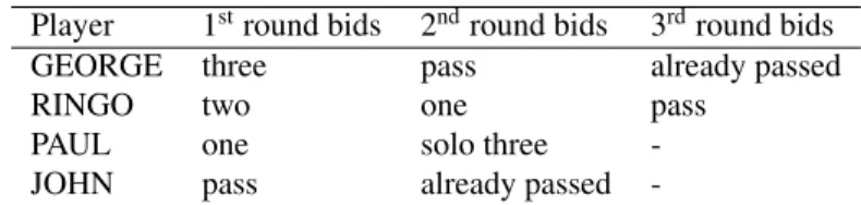
Player 1stround bids 2ndround bids 3rdround bids
GEORGE three pass already passed
RINGO two one pass
PAUL one solo three
-JOHN pass already passed
-Table 2: An example of bidding.
– solo three (40), solo two (50), solo one (60), solo zero (80): the corresponding number of cards is exchanged with talon. The declarer plays alone.
An example of bidding in a four-player tarok game is presented in Table 2. The hands of all players are presented in Table 2. The symbolT stands for trumps called taroks, Hstands for hearts,Cfor clubs,Dfor diamonds andSfor spades. AbbreviationsK, Q, CandBmean the cards king, queen, cavalier and boy respectively.
In the example bidding, Paul holds the strongest cards followed by Ringo and George with John having the weak-est hand. Bidding begins with George, who bids ‘three’, which is obligatory for the first bidder. Ringo bids higher choosing ‘two’. Paul raises to ‘one’. John passes. At the beginning of round two George passes also. Ringo esti-mates that his advantage over Paul is high enough, so he continues bidding. Since his first bid was before Paul’s first bid, the rules of tarok allow him to continue with the same bid as Paul. Paul decides that he can play a solo game and raises to ‘solo three’. In the third round Ringo passes also, which ends the bidding. Paul becomes the declarer. Note that the described bidding for all players was performed by our Tarok7 program.
The strategy of a bidder is to choose the most appropri-ate bid according to the strength of his hand and the esti-mated strength of his partners and opponents. Generally, the types of games associated with high bids require the bidder to have a higher advantage over the opponents to win the game. The strength of the opponents can be esti-mated from their previous bids. Another important task for the bidder is to find an appropriate level of risk. Prior esti-mates of the quality of other players from previous games must also be considered.
In general, there are two ways of solving bidding prob-lems: knowledge-based and simulation-based approaches. In knowledge-based systems prior human knowledge serves as the basis for decision making. A knowledge base can be represented by a hand-crafted set of bidding rules, a decision structure built manually or with help of various
machine learning algorithms. Simulation-based systems use game search. A bid determines the type of game to be played. When a bidder has to make a decision, the system internally simulates several games for each bid. Simulation yields expected final scores for each bid and the bid which leads to the best score is chosen by the bidder.
The advantages of knowledge-based systems are in their better explicability. Decisions of simulation-based systems usually cannot be easily understood and consequently these systems are difficult to modify. Another advantage is the speed of the decision process. In highly complex non-perfect information games simulation-based systems con-sume a lot of time. Since the amount of time to make a decision is limited in real games, usually the number of simulated games has to be reduced. This directly affects the quality of decision making.
On the other hand it is a lot easier to build a simulation-based system, because no knowledge acquisition and im-plementation is needed. The game program that plays the part of the game following bidding itself can be used as a simulation engine. A system using simulation is not con-fined to hard-coded knowledge and can adapt to new oppo-nents easily. Simulation can also find solutions which were not foreseen by the designer of a knowledge-based system.
3 Related Work
is Bridge Baron, described in [15], where authors do not discuss bidding. There are also some other programs for playing bridge such as Quick bridge [12] and Q-plus bridge [13]. Due to their commercial nature it is not know publicly how they work.
Whistis also a card game that includes bidding. [7] de-scribes a program for playing whist that uses game search for card play. Experiments to perform bidding with simula-tion have been performed. The author reports poor results so bidding was not included in the program. Two further examples of programs for playing whist, both commercial, are Bid Whist [2] and Nomination Whist [11].
Betting inpokeris also a form of bidding. Poki, a pro-gram for playing poker described in [1] bases its decisions on simulation aided by statistical modelling of opponents. The program Monash BPP [8] uses Bayesian networks to represent (i) the relationships between current hand type, (ii) final hand type after the five cards have been dealt and (iii) the behaviour of the opponent. Thus the posterior probability of winning a game is obtained. The approach to playing poker that has had most success lately is approxi-mating game-theoretic optimal strategies. It is used by both PsOpti [3], the successor of Poki, and GS2 [4].
Another game that includes bidding is three-player
tarok. Silicon tarokist, a program for three-player tarok de-scribed in [9, 16], also employs simulation for bidding.
4 Complexity of Games with
Bidding
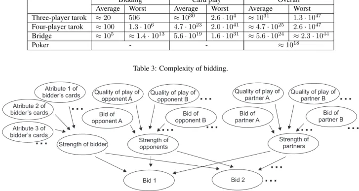
Average and worst-case complexity of different games are presented in Table 4. In general, complexity is measured by the number of possible courses of a game. Tarok and bridge are split into two parts: bidding and card play. We consider card play in tarok to include the part of the game imme-diately following bidding: choosing a partner (four-player tarok only), exchanging cards with talon, announcements and counter-announcements. A game of poker is treated as a whole.
Theaverage complexity of biddingin four-player tarok and bridge was approximated by the average number of real-game choices to the power of the average length of bidding process. The source of data for all the categories, average and worst-case, for three-player tarok is [9]. The source of data for four-player tarok were several hundreds of games played by the Tarok7 program, while for bridge we examined several tens of games played at World Cham-pionships in Montreal, Canada in 2002 [17].
Theworst-case complexity of biddingwas calculated by taking into account all bids allowed by the rules. We cal-culated the worst-case complexity of bidding in bridge and four-player tarok with a special-purpose program. Bidding is most complex in bridge and least complex in three-player tarok.
Thecomplexity of card playin four-player tarok was cal-culated according to the same principles as in three-player
tarok. The average complexity was again computed from several thousands of games of Tarok7 program, while the worst-case complexity was calculated by constructing such hands of cards that yield the largest number of possible courses of card play allowed by the rules. The source of figures for bridge is [15]. Card play is most complex in three-player tarok and least complex in bridge.
The overall complexityof a game is the product of the complexity of bidding and card play. The least complex game according to [1] is poker.
Since we are dealing with imperfect information games, simulation is even more difficult than the figures in Ta-ble 4 suggest. In bridge this is somewhat alleviated by the fact that one player’s cards are visible to all others. In four-player tarok, there is even more uncertainty at the time of bidding since the declarer’s partner is only re-vealed during card play. In addition, the complexity of card play in tarok is significantly higher than the complexity of card play in bridge and the overall complexity of poker. Since using simulation for bidding means that several en-tire games have to be played out, this approach, while suc-cessful in bridge and poker, might not be suitable for tarok. A knowledge-based approach might be more appropriate than simulation.
5 Decision Model for Bidding Using
Bayesian Networks
5.1 Bayesian Networks
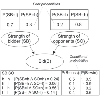
Figure 1: An example Bayesian network.
com-Bidding Card play Overall
Average Worst Average Worst Average Worst
Three-player tarok ≈20 506 ≈1030 2.6·104 ≈1031 1.3·1047 Four-player tarok ≈100 1.3·106 4.7·1023 2.0·1041 ≈4.7·1025 2.6·1047 Bridge ≈105 ≈1.4·1013 5.6·1019 1.6·1031 ≈5.6·1024 ≈2.3·1044
Poker - - ≈1018
Table 3: Complexity of bidding.
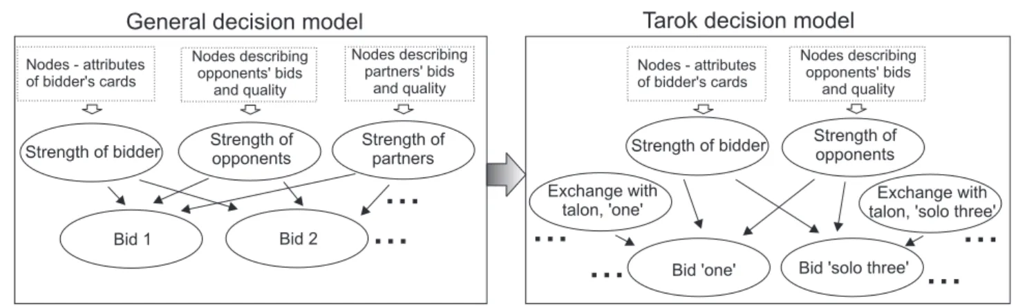
Figure 2: Decision model for bidding using Bayesian network.
monly used when dealing with probabilistic events [14, 6]. An example in Figure 5.1 illustrates an application of Bayesian networks in bidding. The network represents a particular situation from bidding, where the bidder has to decide whether a certain bid is suitable, i.e. whether it is ex-pected to win the game associated with the bid or not. The bidder estimates his strength and the strength of the oppo-nents. The top-level nodes represent the bidder’s knowl-edge about his strength and the strength of the opponents. The bottom-level node represents the expected final result of the game.
With each node one random variable is associated. Each of the variablesSBandSOcan have two values: ‘high’ (h) and ‘low’ (l). The variableBcan have the valueswinand
loss. For example, in our case the bidder estimates that the opponents’ strength is high with probability 0.8. The links between the nodes determine the way the probabilistic vari-ables are conditionally related. In the conditional probabil-ity table (CPT), there are the conditional probabilities that quantify the relation between the random variables. They are set by the designer of the network, and together with the structure of the network reflect the general knowledge about bidding. At the time of bidding decision, prior prob-abilities in top level nodes are set according to the current state of the game and the probabilities of loss and win are computed by Equation 1.
If loss is more probable than win, this bid should not be chosen. In this particular case the probability of a win would be 0.37, which indicates that the bid might not be sensible.
P(B=win) =P(B=win|SB =h, SO=h)
·P(SB=h∧SO=h) +P(B=win|SB =l, SO=h)
·P(SB=l∧SO=h)
+P(B=win|SB =h, SO=l)
·P(SB=h∧SO=l) +P(B=win|SB =l, SO=l)
·P(SB=l∧SO=l)
(1)
5.2 Description of the Model
The knowledge-based decision model for bidding is pre-sented in Figure 5.1. The top-level nodes represent the state of the game at the moment when a player has to make a bid. The mid-level nodes semantically integrate the attributes in the top-level nodes. They are not strictly necessary, but they make the network more compact and easier to design. Each bottom-level node represents one of possible bids and therefore the type of game associated with that bid. The random variables associated with the bottom-level nodes represent the final scores of the game.
P(B=vb) = (2)
X
j1=1...n1,...,jk=1...nk
P(vb|M1=vMj11, . . . , Mk=vMkjk )P(M1=vjM11). . . P(Mk=vMkjk )
P(N =pa) = 0, P(N =l) = 0, P(N =h) = 1. Proba-bilities of the other top-level nodes are set in the same way. Posterior probabilities of the values in the bottom-level nodes are calculated according to the inference rules of Bayesian networks. The values of the bottom-level nodes are assigned discrete numeric values ranging from -1 to 1. Expectations of probability distributions of bottom-level nodes are calculated. The bid that is associated with the highest expectation is chosen. If all expectations are nega-tive, pass is the reasonable choice. The algorithm for deter-mining the optimal bid with the Bayesian network is pre-sented in Figure 5.2
The particular structure of the Bayesian network allows us to use an adapted version of general inference rules. Let vb be a value of a bottom-level node B. LetM =
{M1, M2, ..., Mk}be the set ofkparent nodes of the node
B. LetVmi={v1Mi, ..., vniMi}be the set ofnivalues of the parent nodeMi.P(B =vb)is then calculated by Equation (2). Probabilities of mid-level nodes are calculated recur-sively with the same formula.
5.3 Tuning the Decision Process
The model incorporates three essential factors of bidding decisions: (i) the strength of players (in the mid-level nodes, which summarise bidder’s cards and previous bids of other players), (ii) the values of the types of the games associated with bids and (iii) the level of risk. The second and the third factor are incorporated in the probability dis-tributions in the CPTs of the bottom-level nodes.
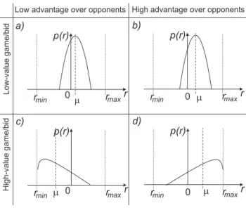
Figure 4: Four basic cases of probability distributions in the bottom-level nodes.
Figure 5.3 illustrates how the model deals with the fac-tors (i) and (ii) with four simple cases regarding the advan-tage of a bidder over his opponents (low/high; i) and the game value (low/high; ii). Each of the probability density functions represents the discrete probability distribution in a bottom-level node, as calculated in the decision process. To make the example more informative we present it using continuous values, although discrete values are used in the real model.
On the horizontal axisrthere are expected game scores. The lower and the upper score limits are denoted byrmin and rmax. Probability density functions associated with these scores are on the vertical axes and are denoted by
p(r). The expectations are denoted byµ. Note that this is only a schematic representation of probability distribu-tions and that actually the following equation would have to hold:
Z rmax
rmin
p(r)dr= 1
Two decision situations are depicted in Figure 5.3. In the left column, the bidder and his partner are slightly stronger or at least not much weaker than the opponents; in the right column the bidder estimates that together with the partner they possess much better cards than the opponents. In both situations the bidder can choose a low-value bid where low negative or positive scores are expected, a high-value bid with high scores expected or pass.
The bidding decision is performed in two steps: First, a particular situation, e.g. ‘Low advantage’ is determined. Then,µfor the low-value bid (a) andµfor the high-value bid (b) are computed. The bidder will evidently choose the bid corresponding to higher value of µ. Ifµis negative, pass is the reasonable choice.
Over multiple games, e.g. in the course of a tournament, new information is obtained to change the bidder’s strategy. This can be easily modelled by modifying the probability distributions in the CPTs of the bottom-level nodes, making bidding more or less aggressive. An example in Figure 5.3 shows two distributions, encouraging less (a) or more (b) risky bidding.
* B: {BID1, BID2,..., BIDn}
* Expect: array [1..n]
* #Array of expectations of probability distributions for each bid
* PostrProb(value)
* #Function calculates the posterior probability of a value
*
* Set values of top-level nodes
* foreach BIDi ∈ B
* foreach value of BIDi
* Expect[BIDi]:= v · PostrProb(value) + Expect[BIDi]
*
* if ∃ BIDi ∈ B such that Expect[BIDi]>0
* choose BIDi: ∀ BIDj ∈ B: Expect[BIDi] >= Expect[BIDj]
* else
* pass
Figure 3: The optimal bid algorithm with Bayesian network.
Figure 6: Bidding decision model for four-player tarok.
Figure 5: Modelling of risk.
5.4 Implementation of the Model for
Four-Player Tarok
To evaluate the decision model we derived a special imple-mentation of it for bidding in four-player tarok as presented in Figure 5.4. Only mid-level and bottom-level nodes are presented in detail. The tarok decision model is part of Tarok7 program.
The top-level nodes are presented as groups (‘Nodes-attributes of bidder’s cards’,...). In the tarok decision model
on the right side of Figure 5.4, these nodes represent con-crete attributes of bidder’s cards and previous bids of other players.
In four-player tarok partners and opponents are not known at the time of bidding. This makes modelling part-ners’ and opponents’ strength more difficult. To simplify the decision process we have decided to omit the nodes de-scribing bids of partners in the tarok decision model. The strength of other players is thus reflected in the nodes de-scribing opponents.
The node ‘Strength of bidder’ can have five values rang-ing from ‘very low’ to ‘very high’. The node ‘Strength of opponents’ can have the values ‘low’ and ‘high’. Imme-diately after bidding, exchange of cards with talon - a set of six cards - is performed by the bidder. Seven special-purpose nodes ‘exchange with talon X’ were added to the model related to exchanging cards with talon. They can have values ‘not suitable’, ‘suitable’, ‘very suitable’. These nodes do not influence the bidder’s strength directly.
SOB SOP EW T P(HD) P(MD) P(MW) P(HW)
VL H S 70 30 0 0
VL H VS 65 35 0 0
L L NS 50 39 11 0
L L S 45 43 12 0
L L VS 40 47 13 0
L H NS 65 34 1 0
L H S 60 38 2 0
L H VS 55 42 3 0
M L NS 55 10 5 30
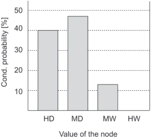
Table 4: CPT of the node ‘Bid solo three’.
Figure 7: Graphical representation of a conditional proba-bility distribution.
win’. In order to calculate expectations of scores for each bid, the values are assigned the numbers -1, -1/3, +1/3 and 1, respectively. In total in the tarok decision model there are seven nodes of the type ‘exchange with talon X’ and seven bottom-level nodes representing bids. Only two of each type are presented in Figure 5.4.
In Table 5.4 we present a part of the CPT of the node ‘Bid solo three’. The first three columns represent con-ditions ‘Strength of bidder’, ‘Strength of opponents’ and ‘Exchange with talon’ with their possible values. The other four columns represent the conditional probabilities of the values of the node expressed in percentages. A simplified way of understanding, for example, of the fifth row of this CPT would be: if strength of the bidder is low, strength of the opponents is also low and exchange of cards with talon is very suitable, then the probability of a high de-feat, moderate dede-feat, moderate win and high win are 40%, 47%, 13% and 0%, respectively. The first 4 and the last 17 rows of the CPT with values of the conditionSOB ‘VL’, ‘M’, ‘H’ and ‘VH’ are missing. The conditional probabil-ity distribution for the fifth row is presented graphically in Figure 5.4. This is a concrete example of the case which is presented schematically in Figure 5.3 c).
6 Simulation
Another approach to bidding is simulation. To estimate whether a bid is suitable, the bidder internally simulates
the part of the game following bidding assuming that he won the bidding and the type of game associated with his bid is played. The problem is that the bidder does not know the cards of the other players. In the case of known cards of the other players it would theoretically be possible to generate all the possible moves for each of the other play-ers and build the whole game tree. The final outcome of each bid could then be determined exactly. However, such an approach is practically impossible due to far too many possibilities.
Monte Carlo method makes simulation reasonably effi-cient, meanwhile retaining its statistical significance. Sev-eral games are internally simulated by the bidder, all start-ing at the end of biddstart-ing assumstart-ing that the bid under con-sideration was successful. Each game the other players are dealt a randomly selected set of cards excluding those in the bidder’s hand. Over many games a statistically signifi-cant distribution of cards can be achieved. The more games are simulated, the more representative are the results.
In the program Tarok7 we also implemented simulation for bidding decisions. The bidder simulates other players using the same strategy he does. Since simulation is time consuming, we combined it with the tarok decision model described in Section 5.2. The bidder first uses the tarok decision model to calculate the expectations of the game scores for each bid allowed by the rules. Then the bidder runs a simulation of 10 games for those 3 bids which ap-peared the most promising according to the decision model. The bid that yields the best results in simulation is chosen at the end. If all bids result in a negative average score, pass is the reasonable choice for the bidder. In Figure 6 the simulation algorithm is depicted.
7 Evaluation
For evaluation purposes we used the Tarok7 program. Bid-ding was implemented with the tarok decision model de-scribed in Section 5.2. Card play was realised with the min-imax algorithm [10]. We performed three tests described in the following sections.
7.1 Bidding with Simulation
In this test we compared our knowledge-based decision model and simulation at bidding. The basis for compari-son of the approaches was their impact on the final game score. The test was performed with four computer play-ers: one of them was normal, while the other three were perfectly informed players (PIP). A PIP in our case uses the same playing strategy as the normal player, but during card play he can see the cards of the other players. Thus, he actually plays a perfect information game and therefore provides a stable reference point. The player observed in the test was the normal player compared to the PIP imme-diately succeeding it in the order of card play.
* B: {BID1, BID2,..., BIDn}
* InitExp: array [1..n];
* FinalExp: array [1..3];
* tarok_dec_model(params. of current game state);
* # Function returns expectations for all possible bids
* simulate_game(bid)
* # Function simulates one game. It returns weighted
* # game score in the interval [-1,1]
*
* InitExp:= tarok_dec_model(params. of curr. game state)
* Bsim ⊂ B such that
* |Bsim| = 3 and
* ∀BIDi ∈ Bsim, ∀BIDj ∈ B-Bsim: InitExp[BIDi]>=InitExp[BIDj]
*
* foreach BIDi ∈ Bsim
* foreach [1..10]
* FinalExp[BIDi]:= simulate_game(BIDi)/10 + FinalExp[BIDi]
*
* if ∃BIDi ∈ Bsim such that FinalExp[BIDi]> 0
* choose BIDi: ∀BIDj ∈ Bsim: FinalExp[BIDi]>=FinalExp[BIDj]
* else
* pass
Figure 8: Simulation algorithm.
First the tarok decision model was used to calculate the ex-pectations of the game scores for each possible bid. Then, simulations of 10 games for the three most promising bids were run. From the results of the simulation another set of game score expectations was calculated. The results of simulation and the decision model were then combined to yield the final decision.
Let us illustrate these calculations with an example. Sup-pose that the decision model yielded the following game score expectations (µm): 0.15, 0.25, 0.28, 0.30, -0.1, -0.3 and -0.8 for the bids ‘three’, ‘two’, ‘one’, ‘solo three’, ‘solo two’, ‘solo one’ and ‘solo zero’, respectively. Note that the value -1 means the highest possible defeat and the value 1 the highest possible win. Then simulations were run for the bids ‘two’, ‘one’ and ‘solo three’, which resulted in expec-tations (µs) 0.28, 0.31 and 0.25. Expectationsµmandµs were then combined with a special coefficientkswhich de-termined the weight of simulation in the decision process. The greater the coefficient, the greater the influence of the simulation. Final expectationsµwere then calculated by the formula: µ = ksµs+ (1−ks)µmLetksin our case be 0.7. This means that the bidder chose the bid ‘one’ with the greatest final expectationµ= 0.30.
In Table 7.1 we present the results of the test. We con-ducted five experiments. In experiment A simulation was not included and 30,000 complete games, bidding and card play were played. In each of the other experiments only 1,000 complete games were played, because simulation is a time consuming process. In each experiment we chose a different value forkswhich is written in the first row. This
Experiment A B C D E
ks 0 0.25 0.5 0.75 1
pc−ph 2.0 2.2 3.4 3.7 3.6
Table 5: Simulation in the decision process at bidding.
way we changed the influence of simulation. In the second row is the measure of quality of play which we calculated the following way: for each experiment we determined two values: (i) the average number of points per game achieved by the normal playerphand (ii) the PIP immediately suc-ceeding the normal playerpc. The measure of the quality of the normal player is the differencepc−ph. The smaller the difference, the better the play.
When comparing results of experiment A to the result of any other experiment, standard error equals approximately 1. We can thus conclude with more than 67% certainty that player A is better than players C, D and E. Comparison with player B is not statistically significant. The results of the test show that in our case it is not sensible to use simu-lation for making bidding decisions. One possibility to get better results would be to significantly increase the number of simulated games. This probably would not be feasible in practice because of the response time constraints.
7.2 Estimating the Optimal Risk at Bidding
Experiment A B C D E F
w/d 0.75 0.73 0.65 0.64 0.60 0.57
pc−ph 3.1 2.5 2.0 2.0 2.5 2.9
Table 6: Estimating optimal level of risk.
test described in Section 7.1: four computer players, three of them were PIPs, the fourth one was a normal player. We observed the quality of play of the normal player and com-pared it to the PIP immediately succeeding it in the order of card play. The normal player was evaluated under dif-ferent risk strategies. The test consisted of six experiments. In each of them the normal player played with different risk at bidding. Setting the risk is described in Figure 5.3. Meanwhile, the PIPs were always the same. In each exper-iment 30,000 complete games, bidding and card play, were played.
The results of the experiments are presented in Table 7.2. The level of risk is shown in the first row as the ratiow/d, wheredis the number of games where the normal player was the declarer, andwis the number of these games that he and his partner also won. The measure of the quality of the normal player shown in the second row ispc−phand was calculated the same way as in the test in Section 7.1.
The standard error of the difference between the average scores per experiment is 0.25. Statistically one can be 95% sure that the normal players in the experiments C and D play better than those in B and E, and more than 99% sure that they play better than the normal players in A and F. It seems that the bidding parameters of normal players in the experiments C or D are close to optimal.
It is worth mentioning that the level of risk which ap-pears to be the best in the test can only serve as an estimate in real games where the opponents are also normal players. In fact, it is impossible to find a particular level of risk that would always be appropriate. A player has to adapt the risk to every particular opponents.
7.3 Tarok7 Compared to Human Experts
In this test, four computer players and an expert human player were bidding at the same time. When it was the fourth player’s turn to bid, first the expert made a bid fol-lowed by the fourth computer player. In this way the hu-man and the computer player were put in exactly the same position at bidding.
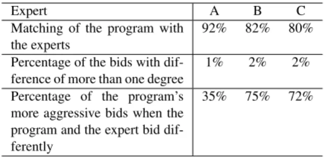
Table 7.3 summarizes the results of the test. Bidding of Tarok7 is compared to three human experts: A, B and C. Expert A made 500 bids, while the other two made 100 bids each. The percentages in the first row denote the pro-portion of bids when the program and the humans chose the same action. The result 100% would mean complete match. The second row represents the cases when the dif-ference between the program’s bid and the expert’s bid was more than one degree, for example, when the program bid ‘three’, and the expert bid ‘one’. For the cases when the
ex-Expert A B C
Matching of the program with the experts
92% 82% 80%
Percentage of the bids with dif-ference of more than one degree
1% 2% 2%
Percentage of the program’s more aggressive bids when the program and the expert bid dif-ferently
35% 75% 72%
Table 7: Comparison of bidding of the Tarok7 program with human experts.
perts and the program bid differently, the fourth row shows the percentages of bids when the program bid higher than the human. The value 100% would mean that the program always bid higher than the expert when they bid differently. Bidding of Tarok7 is more similar to expert A than to the other experts, which was expected since expert A designed the decision model for bidding. According to the results in the fourth row, expert A bid slightly more aggressively than the program, while the other two experts were less aggres-sive. Overall, there are very few cases when the experts and the program disagree strongly in their decisions.
8 Conclusion
In this paper we presented a comparison of two approaches to bidding in four-player tarok one of the most common games in central Europe: the knowledge-based approach and the approach with simulation.
In our tests the knowledge-based model significantly outperformed the simulation. Compared to simulation-based techniques, our decision model offers two additional advantages. First, it does not use any time consuming search for making decisions. This is probably the main reason why it performs better than the simulation. The de-cision model seems to be suitable for any game with bid-ding regardless of how complex its game-play is. Second, the structure of the model is clearly explicable, so it is easy to fine-tune, as we have shown in Section 5.3, when we ex-plained how to achieve the appropriate level of risk. The ca-pacity for fine-tuning and adapting to the opponents could be further exploited by trying to learn the conditional prob-abilities of CPTs automatically. The feedback for a learn-ing algorithm would be bids and scores of games played under these bids.
Other experiments have shown that the program plays quite similarly to human experts and that it is easy to opti-mize for particular opponents. The source code of the de-cision model and the Tarok7 program can be obtained from the authors.
Ex-periments of some other authors [1] indicate that simula-tion might be better for other games.
9 Acknowledgements
The work reported in this paper was supported by the Slovenian Ministry of Higher Education, Science and Technology.
References
[1] D. Billings, A. Davidson, J. Schaeffer, D. Szafron, “The challenge of poker”,Artificial Intelligence Jour-nal, Vol. 134, No. 1-2 , pp. 201-240, 2002.
[2] Bid Whist webpage: http://www.
rwmsoftware.com/
[3] Darse Billings, Neil Burch, Aaron Davidson, Robert Holte, Jonathan Schaeffer, Terence Schauenberg, Du-ane Szafron, “Approximating Game-Theoretic Opti-mal Strategies for Full-Scale Poker”, InProceedings of the International Joint Conference on Artificial In-telligence, Acapulco, Mexico, 2003.
[4] A. Gilpin, T. Sandholm, “A Texas Hold’em poker player based on automated abstraction and real-time equilibrium computation”, inProceedings of the fifth international joint conference on Autonomous agents and multiagent systems, Hakodate, Japan, pp. 1453 -1454, 2006.
[5] M. L. Ginsberg, “GIB: Imperfect information in com-putationally challenging game”,Journal of Artificial Intelligence Research, Vol. 14, pp. 303-358, 2001.
[6] F. V. Jensen, “Bayesian networks and decision graphs”,Springer Verlag: New York, 2001.
[7] J. Fong, “Developing an Artificial Intelligence for Whist”, University of California, Computer Science, Los Angeles, 2005.
[8] K. Korb, A. Nicholson, N. Jitnah, “Bayesian poker”, inProceedings of the 15th Conf. on Uncertainty in Artificial Intelligence, Stockholm, Sweden, pp. 343-350, 1999.
[9] M. Luštrek, M. Gams, I. Bratko, “A program for play-ing tarok”,ICGA Journal, Vol. 23 , No. 3., pp. 190-197, 2003.
[10] D. Marinˇciˇc, “Kombinacija teorije odloˇcanja in preiskovanja pri raˇcunalniškem igranju iger,”Masters thesis, Faculty of computer and information engineer-ing, University of Ljubljana, 2004.
[11] Nomination whist webpage: http://www. nommy.co.uk/
[12] Quick bridge website: http://
wesleysteiner.com/quickgames/ bridge.html
[13] Q-plus bridge website: http://www.q-plus. com/engl/home_f.htm
[14] S. Russel, P. Norvig, “Artificial intelligence: a mod-ern approach”, Prentice Hall, Upper Saddle River, New Jersey, USA, 1995.
[15] S. J. J. Smith, D. Nau, T. Throop, “Computer bridge: a big win for AI planning”,AI Magazine, Vol. 19, No. 2, pp. 93-105, 1998.
[16] Silicon tarokist website. http://tarok. bocosoft.com