PERFORMANCE OF MULTIPLE LINEAR REGRESSION
AND AUTOREGRESSIVE INTEGRATED MOVING
AVERAGE MODELS IN PREDICTING ANNUAL
TEMPERATURES OF OGUN STATE, NIGERIA
1 I. JIBRIL, 2J.J. MUSA, 3P.O.O. DADA, 4H.E. IGBADUN, 1J. M.
MOHAMMED AND H.I. 1MUSTAPHA 1College of Agriculture, P.M.B. 109, Mokwa, Niger State
2Department of Agricultural and Bioresources Engineering, Federal University of Tech-nology, P.M.B. 65, Minna, Niger State, Nigeria.
3Department of Agricultural and Bioresources Engineering, Federal University of Agri-culture, Abeokuta, Ogun State, Nigeria.
4Department of Agricultural and Bioresources Engineering, Ahmadu Bello University, P.M.B. 1044, Zaria, Kaduna State, Nigeria.
*Corresponding author: [email protected] Tel: +2348064485066
ABSTRACT
The performance of Autoregressive Moving Average and Multiple Linear Regression Models in pre-dicting minimum and maximum temperatures of Ogun State is herein reported. Maximum and Mini-mum temperatures data covering a period of 29 years (1982 -2009) obtained from the Nigerian Mete-orological Agency (NiMet), Abeokuta office, Nigeria, were used for the analyses. The data were first processed and aggregated into annual time series. Mann-Kendal non-parametric test and spectral analysis were carried out to detect whether there is trend, seasonal pattern, and either short or long memory in the time series. Mann-Kendal Z-values obtained are –0.47 and –2.03 for minimum and maximum temperatures respectively, indicating no trend, though the plot shows a slight change. The Lo’s R/S Q(N,q) values for minimum and maximum temperatures are 3.67 and 4.43, which are not within the range 0.809 and 1.862, thus signifying presence of long memory. The data was divided into two and the first 20 years data was used for model development, while the remaining was used for validation. Autoregressive Moving Average (ARMA) model of order (5, 3) and Autoregressive (AR) model of order 2 are found best for predicting minimum and maximum temperatures respectively. Mul-tiple Linear Regression (MLR) model with 4 features (moving average, exponential moving average, rate of change and oscillator) were fitted for both temperatures. The ARMA and AR models were found to perform better with Mean Absolute Percentage Error (MAPE) values of -2.89 and -1.37 for minimum and maximum temperatures, compared with the Multiple Linear Regression Models with MAPE values of 141 and 876 respectively. Results of ARMA model can be relied on in generating forecast of temperature of the study area because of their minimal error values. However, it is recom-mended other climatic elements that were not captured in this paper due to unavailability of infor-mation be considered too in order to see which model is best for them.
Keywords: ARMA model, MLR model, Mann-Kendal test, Minimum and Maximum temperatures.
Journal of Natural Science, Engineering
and Technology
ISSN:
Print - 2277 - 0593 Online - 2315 - 7461 © FUNAAB 2017
INTRODUCTION
Temperature is one of the major input vari-ables for land evaluation, characterization systems, hydrological and ecological mod-els. These models use air temperature to drive processes such as evapotranspiration, soil decomposition, and plant productivity (Benavides, et al., 2007). Air temperature is an important site characteristic used in de-termining site suitability for agricultural and forest crops (Benavides, et al., 2007), and it is used in characterizing the habitat of plant species (Rubio, et al., 2002; Sanchez-Palomares et al., 1999) and in determining the patterns of vegetation zonation (Richardson, et al., 2004). Modeling temper-ature therefore, is an important task for effi-cient agricultural development and sustaina-bility.
Models are simplifications of reality that reflect our understanding of the process they represent. Just as any other tool, the results given by models are dependent on how they are applied, and the quality of these answers is not better than the quality of our understanding of the system (Robin, 2003). Some models are based solely on em-pirical equations while others are built on more complex, physically based principles (Butcher, et al., 1998).
One of the most popular and frequently used stochastic time series models for tem-perature analysis is the Autoregressive Inte-grated Moving Average (ARMA) model (Zhang, 2003). The basic assumption made to implement this model is that the consid-ered time series is linear and follows a par-ticular known statistical distribution, such as the normal distribution. ARMA model has subclasses of other models, such as the Au-toregressive (AR), Moving Average (MA) and Autoregressive Moving Average
(ARMA) models (Box et al., 2008). Accord-ing to Box et al., (2008) a quite successful variation of ARMA model, viz; the Seasonal ARMA (SARMA) for seasonal time series forecasting were proposed. The popularity of the ARMA model is mainly due to its flexi-bility to represent several varieties of time series with simplicity as well as the associated Box-Jenkins methodology (Zhang, 2003) for optimal model building process. But the se-vere limitation of these models is the pre-assumed linear form of the associated time series which becomes inadequate in many practical situations.
Also, Multiple Linear Regression models are often used for estimating the future events or values using features of a particular time series or other related time series data (Chatfield, 1994). However, they are more of deterministic, which is unlikely of an ideal situation.
The selection of a proper model is extremely important as it reflects the underlying struc-ture of the series and this fitted model in turn is used for future forecasting. A time series model is said to be linear or non-linear depending on whether the current value of the series is a linear or non-linear function of past observations.
Atmospheric temperature is seen as a major determinant of hydrologic processes. That is, change in temperature level at any point in time leads to change in other climatic ele-ments (Benavides, et al., 2007). Despite this importance of temperature, no literature has shown any work on temperature trend in the study area, and perhaps, if possible make an attempt to build a model and validate. This research paper therefore, intended to check for trend in the temperature time series data, develop and validate a MLR and ARMA
models and as well, compare the perfor-mance of each.
MATERIALS AND METHODS
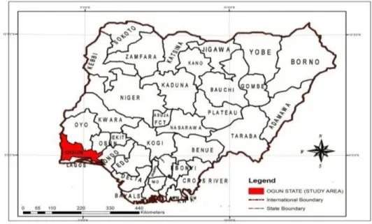
Ogun State is bounded by Oyo state to the north, Osun and Ondo States to the east and Lagos State to the South as shown in (Fig. 1).
It is located in south-western Nigeria, on latitudes 6.260 N and 9.100 N and longitudes 2.280 E and 4.80 E. The land area is about 23,000km2. It is located at an elevation of 77m above sea level. The relief is generally low, with the gradient in the North-South direction (Ewomoje and Ewomooje, 2011). The two major vegetation zones that can be identified in the area are the high forest veg-etation in the north and central parts, and the swamp/mangrove forests that cover the southern coastal and floodplains, next to the lagoon. It has two distinct seasons throughout the year. The monthly rainfall distribution in the study area shows a
dis-tinct dry season extending from November through March and a rainy season divided into two periods: April – July and September – October. The mean annual rainfall data for 30 years showed a variation from about 1,150mm in the northern part to around 2,285mm in the southern extremity. The esti-mates of total annual potential evapotranspi-ration have been put between 1600 and 1900mm. (Ewemoje and Ewemooje, 2011). Data Collection and Preprocessing
The minimum and maximum temperature data used for this study were obtained from the Nigerian Meteorological Agency (NiMet), Abeokuta office, Nigeria. The data collected are the time series type, on monthly bases for a period of 29 years (1982-2009), with the aid of Global Position System (GPS) equipment. For the purpose of this study, the data are pre-whitened and mean annual values were first determined before use.
The Mann-Kendall test was carried out in accordance with the works of Otache et al., (2011); Edwin and Otache, (2014) and Chatfield (2004), with the aid of the excel template of ‘MAKESEN’s version 1. Lo’s modified re-scaled (R/S) test was also done to ascertain if the trend persisted in accord-ance with the works of Robinson, (2003) and Palma, (2007). To check for serial cor-relation, the Durbin-Watson test was
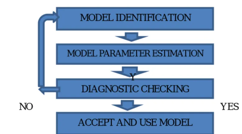
con-sidered in accordance with the works of Christian, (2006); Richard, (2015) and Rama-nathan, (2002). The tests were carried out in order to make sure the time series data con-forms to the basic criteria for stochastic modeling. There is no clear seasonal nature in the time series, therefore, only the sto-chastic component was considered and the Box-Jenkins methodology was applied in the model building as described by Figure 2.
Test for Trend, Long-range Dependency and Serial Correlation
Time series data are generally represented in the form:
1 Where, (t) = Time series
= trend component = Periodic component = Stochastic component
In order to check for the stationarity of the data, the following equations were considered:
2 Where, Xj and Xk are the annual values in years j and k, j > k, respectively, and
3
4 Where, q is number of tied groups and tp is number of data values in the pth group. The
val-ues of S and Var(S) were used to compute the test statistic Z as follows
Based on the fact that the ACF and PACF diagrams are sometimes difficult to inter-pret (Kumar and Vanajakshi, 2015), the iter-ative techniques was utilized, and best
mod-el order determined by the Akaike Infor-mation Criterion (AIC) test in accordance with the works of Kumar and Vanajaksh (2015).
MODEL PARAMETER ESTIMATION
DIAGNOSTIC CHECKING Y
ACCEPT AND USE MODEL MODEL IDENTIFICATION
NO YES
Figure 2: Flow chart of ARMA Model Building Procedures
Features of Annual Temperature Determined for MLR Models
Moving Average (MA): It was calculated progressively according to the equation: 6 Exponential Smoothening (ESM): It was also determined in accordance with (NOHC, 2012). Using the equation:
7
Where;
Ft+1 = forecast of the time series for period t+1
Yt = actual value of the time series in period t
Ft = forecast of the time series for period t.
α = is called the smoothing constant having value (0 ≤ α ≤ 1).
Oscillator (OSC): Oscillator was calculated using either equations 8 and 9. 8 9 Where, N1and N2 are different periods and N1 > N2.
Rate of Change (ROC): It was determined by:
100 10
Where,
dt = the value of the time series at present time t
Using the features or predictors determined as in Tables 4 and 5, Multiple Linear Re-gression (MLR) equations were developed using the first part of the features; and the remaining was used for testing the validity. Microsoft Excel 2010 version and Minitab version 16 were used to process the data.
RESULT AND DISCUSSIONS
ARMA Model Building for Maximum and Minmum Temperature
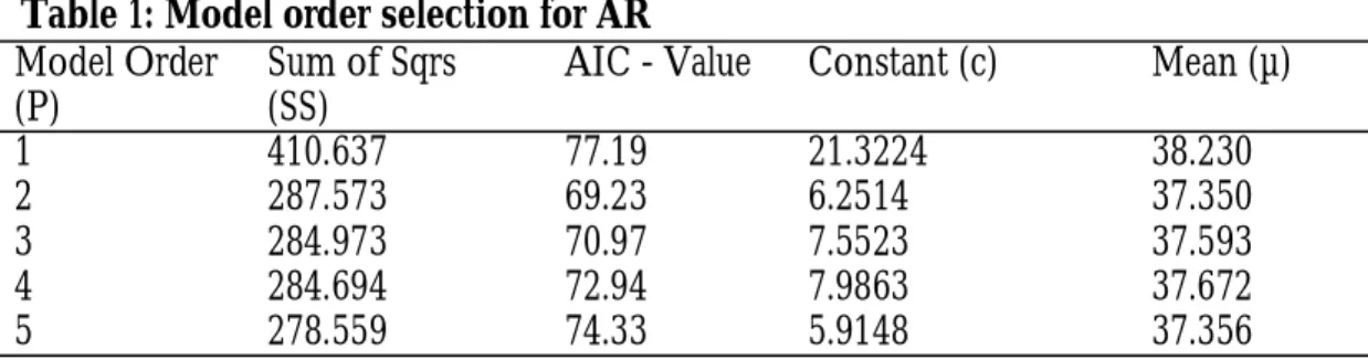
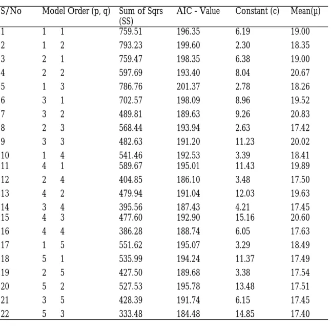
The MannKendal Zvalues of 2.03 and -0.47 were observed for maximum and mini-mum temperatures respectively, which indi-cated no trend in the time series, although, the time series plot shows slight change. Models of order AR (2) and ARMA (5, 3) for maximum and minimum temprture were developed and considered for valida-tion as shown in Tables 1 and 2. The high-lighted (AIC) values in Tables 1 and 2 are the leasts in magnitude when compared with others, this make them the best.
ARMA Model equations developed are
shown in Table 3. They were used to gener-ate forecast for each parameter, and the ac-tual values were ploted with the predicted for validation as shown in Figures 3 and 4 in accordance with the works of Tizro, et al., (2014).
MLR Model Built for Maximum and Minmum Temperature
The features obtained are as shown in Tables 4 and 5. The magnitude of the value of actu-al data is observed to be higher than the pre-dicted values due to the use of 6-year mov-ing average that were considered for both minimum and maximum temperatures. MLR models developed were as shown in Table 6. Temperatures were represented by Y1 and Y2 while, X1, X2, X3 and X4 are the moving average, exponential smoothening, oscillator and rate of change respectively. The plots of actual and predicted values of Minimum and Maximum temperatures for MLR models developed were as shown in Figures 5 and 6. Comparing the Performance of the two Models
The comparism was based on Lewi’s error scaling, which considers the least value of Mean Absolute Percentage Error (MAPE). Best models for minimum and maximum temperatures are respectively Autoregressive Moving Average (ARMA) model of order (5, 3) with Mean Absolute Percentage Error (MAPE) value of -2.89 and Autoregressive (AR) model of order (2) with Mean Absolute Percentage Error (MAPE) value of -1.37, compared with the MAPE values of 141 and 876 obtained from the Multiple Linear Re-gression (MLR) models.
Table 1: Model order selection for AR
Model Order (P)
Sum of Sqrs (SS)
AIC - Value Constant (c) Mean (µ)
1 410.637 77.19 21.3224 38.230
2 287.573 69.23 6.2514 37.350
3 284.973 70.97 7.5523 37.593
4 284.694 72.94 7.9863 37.672
Table 2: Model order selection for ARMA
S/No Model Order (p, q) Sum of Sqrs (SS)
AIC - Value Constant (c) Mean(µ)
1 1 1 759.51 196.35 6.19 19.00
2 1 2 793.23 199.60 2.30 18.35
3 2 1 759.47 198.35 6.38 19.00
4 2 2 597.69 193.40 8.04 20.67
5 1 3 786.76 201.37 2.78 18.26
6 3 1 702.57 198.09 8.96 19.52
7 3 2 489.81 189.63 9.26 20.83
8 2 3 568.44 193.94 2.63 17.42
9 3 3 482.63 191.20 11.23 20.02
10 1 4 541.46 192.53 3.39 18.41
11 4 1 589.67 195.01 11.43 19.89
12 2 4 404.85 186.10 3.48 17.50
13 4 2 479.94 191.04 12.03 19.63
14 3 4 395.56 187.43 4.21 17.45
15 4 3 477.60 192.90 15.16 20.60
16 4 4 386.28 188.74 6.05 17.63
17 1 5 551.62 195.07 3.29 18.49
18 5 1 535.99 194.24 11.37 17.49
19 2 5 427.50 189.68 3.38 17.54
20 5 2 527.53 195.78 13.48 17.51
21 3 5 428.39 191.74 6.15 17.45
22 5 3 333.48 184.48 14.85 17.40
Table 3: Best Model Equations obtained for Maximum and Minimum Temperature
S/No Model Type
Model Order
Model Equation 1 AR 2
3 ARMA 5, 3
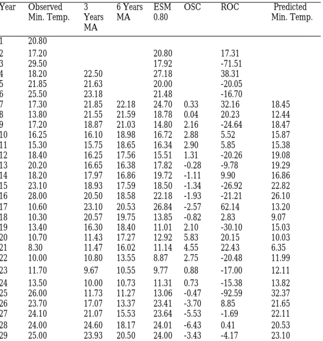
Table 4: Observed values of minimum temperature, features and predicted values of minimum temperature
Year Observed Min. Temp.
3 Years MA
6 Years MA
ESM 0.80
OSC ROC Predicted Min. Temp.
1 20.80
2 17.20 20.80 17.31
3 29.50 17.92 -71.51
4 18.20 22.50 27.18 38.31
5 21.85 21.63 20.00 -20.05
6 25.50 23.18 21.48 -16.70
7 17.30 21.85 22.18 24.70 0.33 32.16 18.45 8 13.80 21.55 21.59 18.78 0.04 20.23 12.44 9 17.20 18.87 21.03 14.80 2.16 -24.64 18.47 10 16.25 16.10 18.98 16.72 2.88 5.52 15.87 11 15.30 15.75 18.65 16.34 2.90 5.85 15.38 12 18.40 16.25 17.56 15.51 1.31 -20.26 19.08 13 20.20 16.65 16.38 17.82 -0.28 -9.78 19.29 14 18.20 17.97 16.86 19.72 -1.11 9.90 16.86 15 23.10 18.93 17.59 18.50 -1.34 -26.92 22.82 16 28.00 20.50 18.58 22.18 -1.93 -21.21 26.10 17 10.60 23.10 20.53 26.84 -2.57 62.14 13.20 18 10.30 20.57 19.75 13.85 -0.82 2.83 9.07 19 13.40 16.30 18.40 11.01 2.10 -30.10 15.03 20 10.70 11.43 17.27 12.92 5.83 20.15 10.03 21 8.30 11.47 16.02 11.14 4.55 22.43 6.35 22 10.00 10.80 13.55 8.87 2.75 -20.48 11.99 23 11.70 9.67 10.55 9.77 0.88 -17.00 12.11 24 13.50 10.00 10.73 11.31 0.73 -15.38 13.82 25 26.00 11.73 11.27 13.06 -0.47 -92.59 32.37 26 23.70 17.07 13.37 23.41 -3.70 8.85 21.65 27 24.10 21.07 15.53 23.64 -5.53 -1.69 22.11 28 24.00 24.60 18.17 24.01 -6.43 0.41 20.53 29 25.00 23.93 20.50 24.00 -3.43 -4.17 23.10
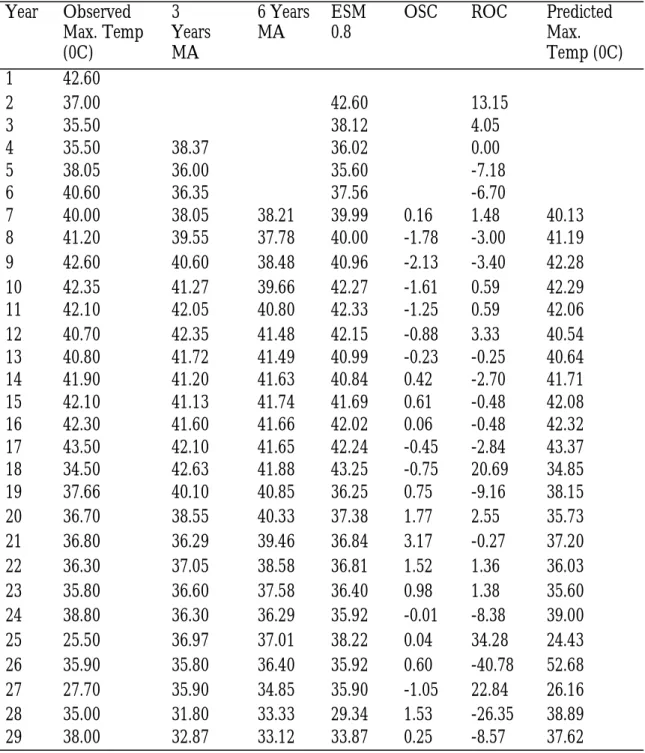
Table 5: Observed values of maximum temperature, features and predicted values of maximum temperature
Year Observed Max. Temp (0C)
3 Years MA
6 Years MA
ESM 0.8
OSC ROC Predicted Max. Temp (0C) 1 42.60
2 37.00 42.60 13.15
3 35.50 38.12 4.05
4 35.50 38.37 36.02 0.00
5 38.05 36.00 35.60 -7.18
6 40.60 36.35 37.56 -6.70
7 40.00 38.05 38.21 39.99 0.16 1.48 40.13 8 41.20 39.55 37.78 40.00 -1.78 -3.00 41.19 9 42.60 40.60 38.48 40.96 -2.13 -3.40 42.28 10 42.35 41.27 39.66 42.27 -1.61 0.59 42.29 11 42.10 42.05 40.80 42.33 -1.25 0.59 42.06 12 40.70 42.35 41.48 42.15 -0.88 3.33 40.54 13 40.80 41.72 41.49 40.99 -0.23 -0.25 40.64 14 41.90 41.20 41.63 40.84 0.42 -2.70 41.71 15 42.10 41.13 41.74 41.69 0.61 -0.48 42.08 16 42.30 41.60 41.66 42.02 0.06 -0.48 42.32 17 43.50 42.10 41.65 42.24 -0.45 -2.84 43.37 18 34.50 42.63 41.88 43.25 -0.75 20.69 34.85 19 37.66 40.10 40.85 36.25 0.75 -9.16 38.15 20 36.70 38.55 40.33 37.38 1.77 2.55 35.73 21 36.80 36.29 39.46 36.84 3.17 -0.27 37.20 22 36.30 37.05 38.58 36.81 1.52 1.36 36.03 23 35.80 36.60 37.58 36.40 0.98 1.38 35.60 24 38.80 36.30 36.29 35.92 -0.01 -8.38 39.00 25 25.50 36.97 37.01 38.22 0.04 34.28 24.43 26 35.90 35.80 36.40 35.92 0.60 -40.78 52.68 27 27.70 35.90 34.85 35.90 -1.05 22.84 26.16 28 35.00 31.80 33.33 29.34 1.53 -26.35 38.89 29 38.00 32.87 33.12 33.87 0.25 -8.57 37.62
Table 6: MLR equation and R- square value obtained for Minimum and maximum temperature
Experiment Regression equation developed R- square value Minimum temperature estimation
using its features
Y2 = - 2.92 - 0.352 X1 + 1.46 X2 + 0.795 X3 - 0.222 X4
0.92 Maximum temperature estimation
using its features
Y1 = - 1.01 - 0.448 X1 + 1.47 X2 + 0.514 X3 - 0.414 X4
0.98
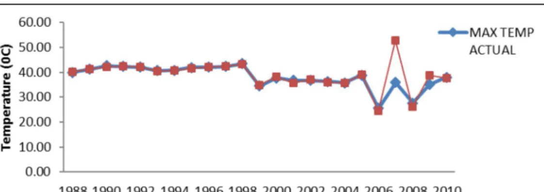
Fig. 3: Actual and Predicted Maximum temperature Plot for AR (2) Model
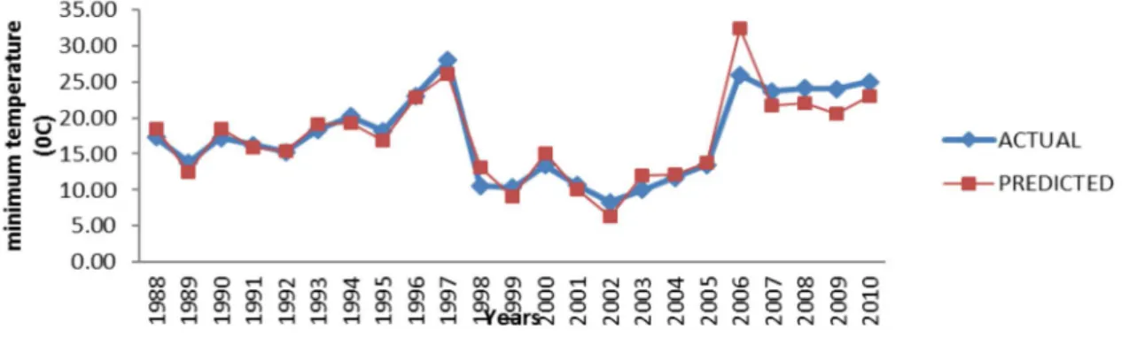
Fig. 4: Actual and Predicted Minimum temperature Plot for ARMA (5, 3) Model
CONCLUSIONS
No trend was established in the temperature time series based on the Mann-Kendal test. The best models for minimum and maxi-mum temperatures are Autoregressive Mov-ing Average (ARMA) model of order (5, 3) with Mean Absolute Percentage Error (MAPE) value of -2.89 and Autoregressive (AR) model of order (2) with Mean Absolute Percentage Error (MAPE) value of -1.37. This best conform to Lewi’s error scaling, compared with the MAPE values of 141 and 876 obtained from the Multiple Linear Regression (MLR) models. The overall results of the best models are prom-ising and could be used for predicting tem-perature in the study area.
REFERENCES
Benavides, R., Fernando, M., Agustin, R., and Koldo, O., (2007). Geostatistical
Modelling of Air Temperature in a Moun-tainous Region of Northern Spain. Agricul-tural and Forest Meteorology (146) 173-188.
Box, G. E. P., Jenkins, G. M., and Rein-sel, G. (2008). Time Series Analysis:
Fore-casting and Control. Wiley, Oxford, 4th Edi-tion.
Butcher, J., Shoemaker, L., Clements, J. T., and Thirolle, E., (1998). Basin
Model-ing Online TrainModel-ing Module. United States Environmental Protection Agency. Basin Academy Web. http://www.epa.gov/ watertrain/modeling.
Fig. 6: Actual and Predicted Maximum Temperature Plot for MLR Model Developed
Table 7: Mean Absolute Percentage Error Values used in Comparing the Models
Model Type Parameter Mode of Comparing Remark AR (2) Max. Temperature MAPE (-1.37) Preferred MLR (Y1) Max. Temperature “ “ (876) Not Preferred ARMA (5, 3) Min. Temperature “ “ (-2.89) Preferred MLR (Y2) Min. Temperature “ “ (141) Not Preferred
Chatfield, C. 2004. The analysis of time
series: An Introduction, sixth edition: New York, Chapman and Hall/CRC.
Christian, H. B., (2006). Measuring Serial
Dependency in Categorical Time Series. Preprint 265. University of Wurzburg.
Edwin, A. I. and Otache, M. Y. 2014
Stochastic Characteristics and Modelling of Monthly Rainfall. Time Series of Ilorin, Ni-geria. Open Journal of Modern Hydrology, 4, 67-79. http://dx.doi.org/10.4236/ojmh. 2014.43006.
Ewemoje, T. A., and Ewemooje, O. S.,
2011. Best Distribution and Fitting Posi-tions of Daily Maximum Flood Estimation at Ona River in Ogun-Osun River Basin, Nigeria. Agricultural Engineering Interna-tional: CIGR Journal. Vol. 13, No. 3.Manuscript No. 1380.
Hamzacebi, C., 2008. ‘Improving
Artifi-cial Neural Networks’ Performance in Sea-sonal Time Series Forecasting’, Information Sciences 178, Pp 4550-4559.
Kumar, V. S. and Vanajakshi, L., 2015.
Short-term Traffic Flow Prediction Using Seasonal ARMA Model with Limited Input Data. Europian Transport Resources Re-view 7:21. DOI 10.1007/s12544-015-0170-8.
Nevada Occupational Health Clinic ‘NOHC’, (2012). Time Series Analysis and
Forecasting: Statistics in Practice. 15(2). Sparks, Nevada.
Otache, M. Y., Ahaneku, I. E. and Mo-hammed, S. A. 2011. ARMA Modelling of
Benue River Flow Dynamics: Comparative Study of PAR Model. Open Journal of
Modern Hydrology, Scientific Research, 1, 1-9.
Palma, W., 2007. Long-Memory Time
Se-ries. John Wiley and Sons Inc., Hoboken, New Jersey, USA.
Ramanathan, R., 2002. Introductory
Econ-ometrics with Applications. 5th ed., Harcourt College Publishers. Chapter 9.
Richard, W. 2015. Serial Correlation: Very Brief Overview. University of Notre Dame.
http://www.nd.edu./~rwilliam.
Richardson, A.D., Lee, X., Friedland, A.J., 2004. Microclimatology of treeline
spruce-fir forests in mountains of the north-eastern United States. Agric. Forest Meteor-ol. 125:53-66.
Robin, P., 2003. Approaching Basin
Model-ing. Streamline Basin Management Bulletin. Vol. 7, No. 3.
Robinson, P. M., 2003. Time Series with
Long Memory. Oxford University Press, Ox-ford.
Rubio, A., Sa´nchez, P. O., Go´mez, V., Gran˜a, D., Elena, R., Blanco, A., 2002.
Autoecology of Chestnut Tree Forest in Cas-tilla, Spain).Investigacio´nAgraria: Sistemas de Recursos Forestales 11 (2), 373–393.
Sanchez-Palomares, O., Sanchez-Serrano, F., Carretero, M.P. 1999. Models
and maps of the climatic variables estimates in peninsular Spain. Madrid, 192 pp.
Sanchez, P. O., Rubio, A., Blanco, A., Elena, R., Go´mez, V., 2003. Parametric
Autoecology of Beech Tree Forest in Castilla y Leon). Investigacio´nAgraria: Sistemas de
Recursos Forestales 12 (1), 87–110.
Tizro, A. T., Ghashghaie, M., Georgiou, P. and Voudouris, K. 2014. Time Series
Analysis of Water Quality Parameters. Jour-nal of Applied Research in Water and
Wastewater 1(1), 43-54.
Zhang, G. P., 2003. Time Series
Forecast-ing UsForecast-ing a Hybrid ARMA and Neural Net-work Model. Neurocomputing (50) 159–175.