Preprint typeset using LATEX style emulateapj v. 05/12/14
THE ORIGIN OF FAINT TIDAL FEATURES AROUND GALAXIES IN THE RESOLVE SURVEY
Callie Hood1
Draft version April 24, 2017
ABSTRACT
We present a study of faint tidal features around galaxies in the REsolved Spectroscopy of a Local VolumE (RESOLVE) survey. Our main sample consists of 1027 galaxies of the RESOLVE survey that overlap with r-band images from the DECam Legacy Survey (DECaLS) which reach a surface brightness limit of 27.9 mag arcsec−2 for a 3σdetection of a 100 arcsec2feature. The images of each galaxy were masked, smoothed, and visually inspected for signs of tidal features such as streams or shells. We find that around 21±2% of the galaxies inspected in the DECaLS images demonstrate this faint substructure with data of this depth, setting a lower limit on the frequency of such features in this sample. We examine the relationship between the presence of tidal features, galaxy characteristics, and environment with several metrics including atomic-gas-to-stellar mass ratio, star-formation history, morphology, distance to nearest neighboring galaxy, and group mass. We find that galaxies with tidal features tend to be gas-rich (G/S > 0.1) and that the tidal features around gas-poor and gas-rich galaxies may have different origins reflected in different trends with star formation, morphology and local environment. We observe that gas-poor galaxies with tidal features have higher stellar masses, closer distances to their nearest neighbors (for neighbors in the same group), and reside in groups with fewer members at a fixed group halo mass when compared to the rest of the gas-poor sample, suggesting the gas-poor galaxies with tidal features may contain a high fraction of galaxies currently interacting or merger remnants. Gas-rich galaxies with tidal features also are closer to their nearest neighbors (for neighbors in the same group) than those without, but also show less bulged morphologies and elevated star formation, suggesting a mixture of tidal features from current interactions, gas accretion, or accretion of small companions below the survey limit.
1. INTRODUCTION
In the paradigm of ΛCDM cosmology, galaxy growth is driven by cosmological gas accretion as well as major and minor mergers. For decades, numerical simulations have shown how baryonic matter can trace these merging events through the formation of discernable tidal features (e.g. Toomre & Toomre, 1972). For example, accre-tion of satellite dwarf galaxies into a larger host galaxy were modeled by Bullock & Johnston (2005), whose sim-ulations according to this model successfully reproduced observed substructure of Milky Way galaxies. Thus, a robust search for these tidal features can help construct a fossil record of the history of recent galaxy accretion events, as well as a test for theories of long-term galaxy evolution.
Though the first simulations that demonstrated the formation of tidal features focused on major mergers, they can also be formed by minor merger events (e.g. Ebrova 2013). Recognition of merging systems based on either direct detection of tidal features or identification of close pairs of galaxies has been used in multiple studies of the merger fraction and rate at various redshifts (Con-selice et al. 2008; Bridge et al. 2010; Lotz et al. 2011). Certain types of tidal features have been connected to particular merging events, such as the proposed origin of tidal tails from wet, major mergers (see Section 5 of Duc et. al. 2015). However, flyby interactions (in which no merger occurs) have also been shown to produce sim-ilar morphological disturbances, complicating the use of
1Physics and Astronomy Department, University of North
Carolina, Chapel Hill, NC 27516, USA
tidal features to identify mergers (e.g. Richer et al. 2003; D’Onghia et al. 2010).
The varied origins of tidal features can also lead to heterogeneous results from attempts to correlate those features with other galaxy properties, such as gas frac-tion, morphology, and star formation history. Simula-tions have shown that galaxy interacSimula-tions can drive the cooling of hot halo gas to provide more fuel to rebuild disks (Moster et al. 2011; Tonnesen & Cen 2012) and have found 20% enhancements in HI fraction among post-merger galaxies (Rafieferantsoa et al. 2014). Some observational studies have shown galaxy interactions can spur the conversion of H1 into HII and the subsequent depletion of gas through star formation (e.g. Lisenfeld et al. 2011; Stark et al. 2013), but Ellison et al. (2015) found no signs of gas-depletion in post-merger systems. The gas content of the galaxies before and after the inter-action affects other parameters as well. A VLA study of 17 close pairs of galaxies has shown a positive correlation between the HI content of a galaxy and the strength of its subsequently triggered star formation (Scudder et al. 2015). Simulations of interactions between high-redshift galaxies, constructed to be gas-rich, have produced con-flicting results; Bournaud et al. (2011) found strong en-hancement in the SFR, Perez et al. (2011) found low-level enhancement, and Perret et al. (2014) found no star formation enhancement due to the interaction.
frac-tions can lead to more spheroidal-like galaxies (Naab et al. 2006; Duc & Renaud 2013), while gas-rich mergers can yield disc-dominated remnants (Lotz et al. 2008; Hopkins et al. 2009a). However, gas accretion can lead to either disks or spheroids depending on the alignment of accreted gas relative to earlier accreted material (Sales et al. 2012). Darg et al. (2010) studied merging galaxies identified through the Galaxy Zoo project and concluded that the effects of mergers on spiral galaxies were much more dramatic (eroding their gas and angular momen-tum supplies and strongly enhancing their SFRs), so dis-turbed spiral galaxies were more easily observable than disturbed ellipticals.
Previous studies have produced discrepant estimates of the frequency of nearby faint tidal features from 12% (Atkinson et al. 2013) to 70% (van Dokkum et al. 2005). These discrepancies most likely stem from differences in detection criteria, sample selection, and surface bright-ness limits. The varied nature of the origin of tidal fea-tures calls for the systematic study of their existence around galaxies in a statistically complete survey for which we can characterize their correlation with gas con-tent and other parameters. In this work, we present a uniform search for faint substructure within the highly complete volume-limited REsolve Spectroscopy of a Lo-cal VolumE (RESOLVE) survey. A census of the low sur-face brightness components of RESOLVE galaxies serves as a basis to investigate key questions about the pres-ence of substructure around galaxies in the local uni-verse: which galaxy parameters in the local universe cor-relate most strongly with tidal features? Are these global trends, or are there separate populations within our sam-ple? Can the environmental dependence of these features illuminate their origins?
This work is structured as follows. Section 2 discusses the data sets used in this work as well as the methods used to identify faint tidal features around our galaxies. Section 3 details the results of our census, characterizing our surface brightness limitations while investigating the relationship of detected features to various parameters recorded by the RESOLVE survey. A discussion of our results is presented in Section 4, and our conclusions are outlined in Section 5.
2. DATA AND METHODS
2.1. The RESOLVE Survey
Our main goal is to detect faint tidal features around galaxies in the RESOLVE survey, a volume-limited cen-sus of stellar, gas, and dynamical mass encompassing more than 50,000 cubic Mpc of the nearby universe (Kan-nappan & Wei 2008). A more thorough description of the survey design will given in S.J. Kannappan et al. (in preparation), but we briefly outline the key aspects of the survey below.
2.1.1. Survey Definition
RESOLVE is split into two equatorial strips, RESOLVE-A and RESOLVE-B. RESOLVE A spans 8.75 hr < R.A. < 15.75 hr and 0◦ < Dec. < 5◦, while RESOLVE-B spans from 22 hr<R.A.<3 hr and -1.25◦
< Dec. < 1.25◦ (overlapping the deep SDSS Stripe-82 field). Both areas are also bounded in Local Group-corrected heliocentric velocity fromVLG=4500-7000 km
s−1. RESOLVE is a baryonic mass limited survey, where
M∗ is the stellar mass, 1.4MHI is the atomic hydrogen gas mass corrected for helium contributions, and we de-fine baryonic mass asMbary=M∗+ 1.4MHI. Both RE-SOLVE regions are initially selected on r-band absolute magnitude since this property tightly correlates with the total baryonic mass (Kannappan et al. 2013). The RE-SOLVE survey makes use of the SDSS redshift survey as well as additional redshifts from the Updated Zwicky Catalog (Falco et al. 1999), HyperLEDA (Paturel et al. 2003), 2dF (Colless et al. 2001), 6dF (Jones et al. 2009), GAMA (Driver at al. 2011), Arecibo Legacy Fast ALFA (Haynes et al. 2011), and new observations with the SOAR and SALT telescopes (S.J. Kannappan et al., in preparation). RESOLVE reaches r-band completeness limits ofMr<-17 for RESOLVE-B andMr<-17.33 for RESOLVE-A, the former limit being fainter as a result of RESOLVE-B’s overlap with the deep Stripe-82 SDSS re-gion. Eckert et al. (2016) estimate the baryonic mass completion limit by considering the range of possible baryonic mass-to-light ratios at the r-band absolute mag-nitude completeness limit, obtaining baryonic mass com-pleteness limits of Mbary= 109.3 M andMbary= 109.1 Min RESOLVE-A and RESOLVE-B, respectively.
One advantage of the RESOLVE survey is the variety of multiwavelength data available. An optical spectro-scopic survey is in progress, mainly with the 4.1 m SOAR telescope, whose observations provide either ionized gas or stellar kinematics in addition to gas and stellar metal-licities. In addition, 21 cm observations presented in Stark et al. (2016) provide a H I mass inventory for RESOLVE galaxies while several overlapping photomet-ric surveys span near-infrared to ultraviolet wavelengths, which are used to estimate stellar masses and colors (Eck-ert et al. 2015).
2.1.2. Custom Photometry and Stellar Masses
A full description of the photometric analysis for RE-SOLVE can be found in Eckert et al. (2015). All avail-able photometric data, including SDSS ugriz (Aihara et al. 2011), 2MASS JHK (Skrutskie et al. 2006), UKIDSS YHK (Hambly et al. 2008), and GALEX NUV (Morris-sey et al. 2007) were reanalyzed with custom pipelines to produce uniform magnitude measurements and improve the recovery of low surface brightness emission. This new uniform photometry was used to calculate stellar masses and other stellar population parameters using the spec-tral energy distribution fitting code described in Kannap-pan & Gawiser (2007) and modified in KannapKannap-pan et al. (2013). Eckert et. al. (2015) uses the second grid from Kannappan et al. (2013), which combines old simple stellar populations with age ranging from 2 to 12 Gyr and young stellar populations described either by con-tinuous star formation from 1015 Myr ago until between 0 and 195 Myr ago, or by a simple stellar populations with age 360, 509, 641, 806, or 1015 Myr. This model grid includes a low-metallicity choice (Z = 0.004) and adopts a Chabrier IMF. Likelihoods and stellar masses are computed for all models in the grid, and the median of the likelihood-weighted stellar mass distribution pro-vides the most robust final stellar mass estimate. These stellar masses are given in Eckert et al. (2015).
the last Gyr to preexisting stellar mass (referred to as the long-term fractional stellar mass growth rate, FS-MGR) as described in Kannappan et al. 2013. Both the likelihood-weighted mean and likelihood-weighted me-dian FSMGR are estimated for each galaxy; for our anal-ysis in Section 3.5, we use the average of these two quan-tities. In addition, the short-term star formation rate of each galaxy is calculated from the NUV GALEX band using the calibration from Wilkins et al. 2012.
2.1.3. HI Masses
The HI mass inventory for RESOLVE is fully described in Stark et al. (2016). That 21 cm data release offers ro-bust detections or strong upper limits (Mgas<0.05M∗) for∼94 % of RESOLVE. The HI masses and upper limits for RESOLVE come from the blind 21 cm ALFALFA sur-vey (Haynes et al. 2011) as well as new observations with GBT and Arecibo telescopes. To increase the yield from the basic ALFALFA data products, Stark et al. (2016) extracted 140 lower S/N detections and upper limits for RESOLVE galaxies within the ALFALFA grids. In addi-tion, they acquired pointed observations with the GBT and Arecibo telescopes obtaining HI data for 290 galax-ies in RESOLVE-A and 337 galaxgalax-ies in RESOLVE-B, targeting those with either no HI measurements or weak upper limits from ALFALFA.
The HI masses and upper limits were measured ac-cording to the algorithms in Kannappan et al. (2013) and Stark et al. (2016). Confused sources were iden-tified based on the telescope used, with a search radius of 40 for the ALFALFA smoothed resolution element, 9 for the GBT, and 3.5 for Arecibo pointed observations. Stark et al. (2016) deconfused the HI profiles when pos-sible, building on the methods used in Kannappan et al. (2013). Overall, the 21 cm survey is ∼ 94% complete (94% in RESOLVE-A, 95% in RESOLVE-B) and>85% complete at all mass scales, where complete is defined by detections with a S/N>5 or an upper limit yielding
MHI/M∗ <0.1. For galaxies with confused detections, without HI observations, or with weak upper limits,MHI is estimated using the relationship between color, axial ratio, and gas-to-stellar mass ratio as calibrated in Eckert et al. (2015).
2.1.4. Environment Metrics
One of the benefits of studying tidal features around RESOLVE is the environmental context provided by the survey. Moffett et al. (2015) identified groups of RE-SOLVE galaxies using the friends-of-friends (FoF) tech-nique described in Berlind et al. (2006). For this work, they used tangential and line-of-sight linking lengths of 0.07 and 1.1 times the mean spacing between the galax-ies to optimize the group-finding procedure as recom-mended by Duarte and Mamon (2014) and confirmed for RESOLVE-A in Eckert et al. (2016). For RESOLVE-B, the volume is too small and subject to cosmic variance to use linking lengths from the survey0s own mean galaxy density. Instead, a RESOLVE-B analog was constructed from the larger Environmental COntext (ECO) cata-log which encompasses RESOLVE-A (see Moffett et al. 2015), enforcing a stellar mass selection limit of 108.7M
to match RESOLVE-B. The authors then determine the physical linking lengths and the relationship between the
group halo mass and stellar mass, which are applied to RESOLVE-B. Eckert et al. (2016) assigned each group a halo mass by halo abundance matching (HAM) with the theoretical halo mass function from Warren et al. (2006) using the total group r-band luminosity (for more details see Eckert et al. 2016).
Furthermore, for each galaxy in RESOLVE, we find nearest neighbors in two ways. First, we perform a cylindrical search for nearest neighbor galaxies also in RESOLVE within a radius of 100 Mpc in the plane of the sky. Candidate neighbors are limited to |Vgal − Vneighbor| ≤ 500km/s, where the local group corrected velocities are used to define galaxy redshift. Second, we also compute the distance to each galaxy’s nearest neighbor using the algorithm described by Maneewong-vatana & Mount (1999) as implemented in cKDTree in the scikit-learn package in Python (Pedregosa et al. 2011). We implement this algorithm by converting RA, DEC, and redshift to physical units both with and with-out peculiar motions (so allowing false ∆z or zero ∆z
within groups). The differences in results obtained from these methods are discussed in Section 3.6.1.
2.2. Image Sources
This project utilizes r-band images from both the DE-Cam Legacy Survey (DECaLS) and the IAC Stripe 82 Legacy Project. The DECaLS survey covers both RE-SOLVE subvolumes, with deep r-band images that yield a median surface brightness limit in areas with 3 ob-servations of 27.9 mag arcsec−2 for a 3σ detection of a 100 arcsec2low surface brightness feature (Schlegel et al. 2015), allowing us to probe the brighter side of tidal fea-tures around RESOLVE galaxies. In contrast, the IAC Stripe 82 Legacy Project provides deep r-band co-adds for only RESOLVE-B, but reaches a surface brightness limit of 28.3 mag arcsec−2 for a 3σ detection of a 100 arcsec2 feature (Fliri & Trujillo 2015). See Figure1 for a side-by-side comparison of the galaxy rf0358 in SDSS, DECaLS, and IAC. Though our analysis mainly focuses on the galaxies inspected with DECaLS images, the IAC co-adds allow for a closer study of the dependence of our classifications on the surface brightness limits of our data.
2.3. Detection Process
Figure 1. A comparison of the SDSS (left), DECaLS (middle), and IAC (right) images of the galaxy rf0358. The deeper DECaLS and IAC images reveal the faint extension on the left side of the galaxy.
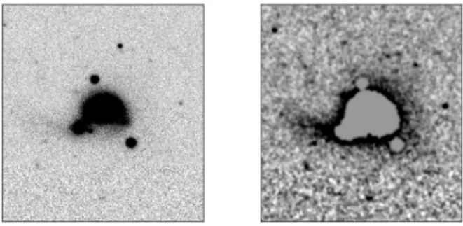
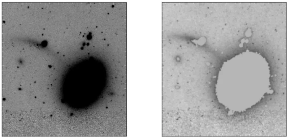
Figure 2. Original DECaLS image of rf0464, as well as the smoothed and masked thumbnail. A tidal stream coming off of the satellite being accreted is enhanced in the smoothed image.
at the beginning of the detection process the sample of galaxies decreased to 1027.
Figure 3. Original DECaLS image of rf0305, which showcases a clear arm arcing above the galaxy. However, this feature is masked out of the smoothed image.
To improve detection of features with particularly low surface brightnesses, each galaxy thumbnail was run through a modification of a previously-developed masking and smoothing code (Ian DellAntonio, private conversation). For each image, Sextractor (Bertin & Arnouts 1996) was used to detect sources within the im-age and use the resulting catalog to create masks. These masks were then subtracted from the original image us-ing IRAF, allowus-ing for only faint and small-scale features to remain. The masked thumbnail was then smoothed with a Gaussian filter in order to enhance these features. One such final image is shown in Figure2, with the faint tidal stream coming off of the smaller galaxy on the left much clearer in the smoothed image. However, while this masking and smoothing process greatly enhanced some of the features, some other substructure was possi-bly masked out in this process as confirmed in the test case shown in Figure3. As a result, both the original and the smoothed, masked images needed to be inspected for
faint tidal features.
For the visual inspection, a code previously used for by-eye morphological classifications of RESOLVE-A galax-ies (see Moffett et al. 2015) was adapted with the APLpy Python package to display images of galaxies as well as images with overlaid contours revealing larger-scale galactic structure. In addition, the masked and smoothed image of each galaxy, as well as the original, were displayed in a DS9 (Joye & Mandel 2003) window to allow for interactive adjustment of the contrast and scaling for each thumbnail. For each of the 1027 galax-ies in the identification sample, a flag was recorded after visual inspection indicating a positive or negative detec-tion of faint tidal features, as well as any comments on particularly interesting substructures.
3. RESULTS AND ANALYSIS
3.1. Frequency of Tidal Features
We find that around 21±2% of the 1027 RESOLVE galaxies inspected with DECaLS have tidal features. Our uncertainty in this value is given due to the range of possible percentages within a two-sided one sigma con-fidence interval given small number statistics. Most of the features detected are thin and small streams as well as bridges to nearby companions; however, some broader faint extensions are detected as well. A selection of fea-tures found around RESOLVE galaxies is shown in the Appendix.
As previously mentioned, past surveys of faint sub-structure do not agree on the frequency of these features; see Table 1 in Atkinson et al. (2013) for an overview of results from published surveys. However, it is difficult to compare these surveys with each other and with the present work due to differences in surface brightness lim-its and sample selection. Atkinson et. al. (2013) were able to detect tidal features around 12% of their 1781 galaxy sample with the strictest confidence; the fraction increased to 18% when including probable but slightly less convincing features. Although their frequency of tidal features is comparable to that presented in this work, Atkinson and colleagues included more broad tidal features than in this paper, including a “miscellaneous diffuse material” category, and were only able to detect tidal features down to 27 mag arcsec−2. Thus, this sim-ilarity could be a result of cancelling effects from these two differences on the number of observed tidal features.
3.1.1. Comparison to Classifications with IAC Stripe 82 Co-adds
For the 446 RESOLVE-B galaxies inspected with both DECaLS and IAC images, we found 20±2% and 24±2% have tidal features, respectively. The difference in fre-quency comes from 18 galaxies whose tidal features are detectable in the IAC co-adds, but not the DECaLS im-ages, most likely due to the ∼ 0.4 mag arcsec−2 differ-ence in surface brightness depth between the two im-age sources. We compared the stellar-mass, color, and gas-to-stellar mass ratio distributions of the two sets of galaxies with tidal features, finding no statistically sig-nificant differences between the two samples according to the Kolmogorov-Smirnov (K-S) test (pKS ∼0.99 for each comparison). Thus, the results presented in the fol-lowing sections would likely not change significantly if we were using classifications from the deeper Stripe 82 co-adds.
3.1.2. Noise Degradation Experiment
In order to further test the dependence of our classifica-tions on the surface brightness limit of our data, we have artificially degraded the IAC images to the same surface brightness limit as our DECaLS cutouts. When we re-classify these noisy IAC images, we find that ∼18±2% of the inspected galaxies host tidal features. We find that 21 of the galaxies classified as having tidal features in the DECaLS images are not similarly classified in the degraded IAC images; conversely, 9 of the galaxies iden-tified with tidal features in the degraded images are not flagged with the DECaLS images. The exact source of these discrepancies is unclear; some of these galaxies have barely discernible tidal features whose classification may have oscillated. We quantify the differences in these clas-sifications with Cohen’s kappa statistic, which is tradi-tionally used to measure inter-classifier agreement while taking into account the probability of classifiers agree-ing by chance. Cohen’s kappa is calculated accordagree-ing to the following formula, where pO is the relative ob-served agreement between classifiers andpeis the hypo-thetical probability of chance agreement. Our DECaLS and noisy IAC classifications have a Cohen’s kappa value 0.79, where values are between -1 and 1 with the maxi-mum reflecting perfect agreement. According to Landis & Koch (1977), our value corresponds to a substantial
−3 −2 −1 0 1 2 3
Log Atomic-Gas-to-Stellar Mass Ratio
0.0
0.1
0.2
0.3
0.4
0.5
0.6
0.7
Probability
Density
pKS= 3.7e−10
With Tidal Features Without Tidal Features
Figure 4. Distributions of gas-to-stellar mass ratio for galaxies identified with tidal features in yellow as well as without tidal fea-tures in purple. These kernel density estimations were created with a Gaussian kernel and a cross-validated optimal bandwidth of h=0.16 dex.
strength of agreement. As in 3.1.1, we do not find any statistically significant differences between the distribu-tions of various parameters (stellar mass, color, etc.) for the galaxies with tidal features from the two imaging sources. Therefore, any marginally detectable tidal fea-tures or false detections should have a minimal effect on the results below.
3.2. Direct Galaxy Properties and Tidal Features
We have examined a multitude of galaxy properties in the RESOLVE catalog to compare their distributions for galaxies with and without tidal features. The most statistically significant difference between distributions is for gas-to-stellar mass ratios (G/S). The G/S distribu-tions for galaxies with tidal features and for those with-out are shown in Figure 4. A Kolmogorov-Smirnov (K-S) test comparing the G/S distributions in Figure 4 yields pKS ∼10−10, meaning the gas fraction distributions of galaxies with and without tidal features would have neg-ligible probability of coming from the same parent dis-tribution. We can see from the figure that galaxies in our sample with tidal features tend to have higher gas fractions; Lotz et al. (2010) found in simulations that galaxy mergers with high gas fractions exhibit disturbed morphologies for longer periods of time than their gas poor counterparts. Thus, it is not necessarily surpris-ing that we tend to find more tidal features in gas-rich galaxies. However, both galaxies with and without tidal features exhibit a modest bimodality in gas fraction, in-dicating that separating our samples into gas-poor and gas-rich galaxies may yield differing results in relation to other parameters. We make this divide at G/S= 0.1, as marked by the dashed line in Figure 4.
Other galaxy properties that produced slightly less strong results were u-r color, FSMGR, and the morphol-ogy metricµ∆introduced in Kannappan et al. (2013) to distinguish quasi-bulgeless (µ∆<8.6), bulged disk (8.6<
features might reflect different formation mechanisms, we decided to look for parameters that might be important without even a simple direct correspondence with tidal features.
3.3. Random Forest Analysis
We applied automated methods to determine which parameters are most important for predicting tidal fea-tures. The Random Forest algorithm (Breiman 2001), implemented in this work with the public Python library scikit-learn (Pedregosa et al. 2011), generates classifica-tions based on a random ensemble of decision trees based on all provided input parameters. From this process, the algorithm also determines the score of the importance of each input feature in the resulting classifications. We trained the algorithm using our by-eye identification of tidal features discussed in Section 2.3. We judged the performance of our classifier with the F1 metric, the har-monic mean of precision (the number of correct positive results divided by the number of all positive results) and recall (the number of correct positive results divided by the number of positive results that should have been re-turned). An F1 score reaches its best value at 1 and worst at 0. The best hyperparameters for our classifier, such as the number of generated decision trees, were op-timized to maximize this F1 metric with ten-fold cross validation (Geisser 1975).
G/S ratio
avg FSMGR
µ∆ nndist
M
∗
r90 r50
absmagr b/a dgr
b/a inner
disk rvir
halo mass
groupcz HIasymm
grpn central
Feature 0.00
0.02 0.04 0.06 0.08 0.10 0.12 0.14
Feature
Importance
Figure 5. Relative importance of each feature inputted into our random forest classifier in predicting whether a galaxy has a tidal feature.The top 5 most important parameters are: G/S ratio, av-erage FSMGR,µ∆, nearest-neighbor distance, and stellar mass. The other correspond to, in decreasing order, 90%-light radius in r band, half-light radius in r band, absolute magnitude in the r band, axial ratio, b/a, (g-r) color gradient, axial ratio of inner disk region of galaxy, virial radius of group, group halo mass, group redshift, HI asymmetry, number of group members, and central status (1 or 0).
The relative contribution of each parameter to our Random Forest classification is shown in Figure 5. Our best-performing Random Classifier only achieved an F1 score of 0.5; however, from the feature selection results of Figure 5, we were able to identify parameters to be further investigated when splitting our sample into gas-poor and gas-rich galaxies. The top five most important features in descending order are as follows: the atomic gas-to-stellar mass ratio, the average FSMGR, the mor-phology metric µ∆, the distance to the galaxy’s near-est neighbor in RESOLVE, and the stellar mass of the
−1.5 −1.0 −0.5 0.0 0.5 1.0 1.5
Log Atomic Gas-to-Stellar Mass Ratio −12.5
−12.0 −11.5 −11.0 −10.5 −10.0 −9.5 −9.0 −8.5
log(
SSFR
y
r
−
1)
pP F F= 3.4e−10
Gas-Rich Galaxies with Tidal Features
0.15 0.30 0.45 0.60 0.75 0.90 1.05 1.20
Density of Gas-Rich Galaxies without Tidal Features
Figure 6. Distributions of specific star formation rate versus gas-to-stellar mass ratio for gas-rich galaxies with (black contours) and without (blue contours) tidal features. The overlaid contours indi-cate the density of gas-rich galaxies with tidal features at the levels 0.15, 0.45, 0.75, and 1.05. Galaxies with tidal features are more concentrated to higher G/S and higher SSFR, showing elevated recent star formation.
−2.0 −1.5 −1.0
Log Atomic Gas-to-Stellar Mass Ratio −12.5
−12.0
−11.5
−11.0
−10.5
log(
SSFR
y
r
−
1)
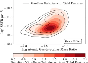
pP F F= 0.1 Gas-Poor Galaxies with Tidal Features
0.3 0.6 0.9 1.2 1.5 1.8 2.1 2.4 Density of Gas-Poor Galaxies without Tidal Features
Figure 7. Distributions of specific star formation rate versus gas-to-stellar mass ratio for gas-poor galaxies with (black contours) and without (red contours) tidal features. The overlaid contours indi-cate the density of gas-poor galaxies with tidal features at the levels 0.3, 0.6, and 0.9. There is not a statistically significant difference between the two distributions as determined by the multivariate K-S test
galaxy. Although stellar mass is less important than the first four, we analyze it to put our results in interpre-tive context. Some of the remaining galaxy properties are also analyzed for similar reasons. Below we analyze the roles of star formation, morphology, stellar mass, and environment in relation to our gas-rich and gas-poor sub-samples.
3.4. Star Formation
To investigate the possible distinct origins of tidal fea-tures in gas-rich and gas-poor galaxies, we looked at the distributions of the star formation metrics discussed in Section 2.1.3. A comparison of the specific star forma-tion rate (SSFR) versus G/S distribuforma-tions for gas-rich galaxies with and without tidal features is shown in
−1.5 −1.0 −0.5 0.0 0.5 1.0 1.5 Log Atomic Gas-to-Stellar Mass Ratio −1.5
−1.0 −0.5 0.0 0.5 1.0 1.5
log(
FSMGR
Gy
r
−
1)
pP F F = 7.8e−09
Gas-Rich Galaxies with Tidal Features
0.1 0.2 0.3 0.4 0.5 0.6 0.7
Density of Gas-Rich Galaxies without Tidal Features
Figure 8. Distributions of fractional stellar mass growth rate versus gas-to-stellar mass ratio for gas-rich galaxies with (black contours) and without (blue contours) tidal features. The over-laid contours indicate the density of gas-rich galaxies with tidal features at the levels 0.1, 0.3, 0.5, and 0.7. Galaxies with tidal features are more concentrated to higher G/S and higher FSMGR, showing elevated long-term star formation.
−2.0 −1.5 −1.0
Log Atomic Gas-to-Stellar Mass Ratio −2.5
−2.0 −1.5 −1.0 −0.5 0.0
log(
FSMGR
Gy
r
−
1)
pP F F= 0.019
Gas-Poor Galaxies with Tidal Features
0.25 0.50 0.75 1.00 1.25 1.50 1.75 2.00 Density of Gas-Poor Galaxies without Tidal Features Figure 9. Distributions of fractional stellar mass growth rate ver-sus gas-to-stellar mass ratio for gas-poor galaxies with (black tours) and without (red contours) tidal features. The overlaid con-tours indicate the density of gas-poor galaxies with tidal features at the levels 0.25, 0.5, 0.75, 1, and 1.25. The galaxies with tidal features are slightly more concentrated to lower G/S and lower FSMGR, but it is not as strong of a result as that shown for the gas-rich galaxies.
in Figure 7. We used the Fasano & Franceschini (1987) variation of the Peacock test (1983), an extension of the K-S test to two dimensions, to determine the statistical significance of the difference between each pair of distri-butions. Within our sample of gas-rich galaxies, those with tidal features appear to be have both larger G/S as seen in Section 3.3 as well as elevated SSFR. In contrast, the presence or absence of tidal features does not corre-spond to a statistically significant difference in the SSFR v. G/S plot for gas-poor galaxies in Figure6.
Furthermore, we created similar plots comparing the FSMGR v. G/S distributions of tidally disturbed galax-ies and their counterparts within the rich and gas-poor samples. Gas-rich galaxies with tidal features have had greater star formation in the past Gyr than those
−1.5 −1.0 −0.5 0.0 0.5 1.0 1.5 2.0
Log Atomic Gas-to-Stellar Mass Ratio 6.0
6.5 7.0 7.5 8.0 8.5 9.0 9.5 10.0
µ∆
pP F F= 3.4e−09
Gas-Rich Galaxies with Tidal Features
0.1 0.2 0.3 0.4 0.5 0.6 0.7 0.8 Density of Gas-Rich Galaxies without Tidal Features
Figure 10. Distributions ofµ∆versus gas-to-stellar mass ratio for gas-rich galaxies with (black contours) and without (blue contours) tidal features. The overlaid contours indicate the density of gas-rich galaxies with tidal features at the levels 0.1, 0.2, 0.3, 0.4, and 0.5. Galaxies with tidal features are more concentrated to higher G/S and lowerµ∆than their counterparts without tidal features, appearing less-bulged with a significance of pP F F ∼10−9.
−2.0 −1.5 −1.0
Log Atomic Gas-to-Stellar Mass Ratio 8.0
8.5 9.0 9.5 10.0 10.5 11.0
µ∆
pP F F= 0.081
Gas-Poor Galaxies with Tidal Features
0.2 0.4 0.6 0.8 1.0 1.2 1.4
Density of Gas-Poor Galaxies without Tidal Features
Figure 11. Distributions ofµ∆versus gas-to-stellar mass ratio for gas-poor galaxies with (black contours) and without (red contours) tidal features. The overlaid contours indicate the density of gas-poor galaxies with tidal features at the levels 0.2, 0.4, 0.6, 0.8, and 1.0. There is not a statistically significant difference between the two distributions as determined by the multivariate K-S test described in section 3.4.
without tidal features as shown in Figure8. Conversely, gas-poor galaxies with tidal features show a slight ten-dency towards lower FSMGRs than their counterparts without tidal features (though at<3σsignificance). Con-trasting results for our gas-poor and gas-rich populations suggest distinct origins for their tidal features.
3.5. Morphology
To examine the relationship of morphology to our gas-rich and gas-poor samples, we use the structure metric
Compar-5 6 7 8 9 10 11 12
Log Stellar Mass (M) 0.0
0.1 0.2 0.3 0.4 0.5 0.6 0.7 0.8
Probability
Density
pKS= 0.19
With Tidal Features Without Tidal Features
Figure 12. Distributions of stellar mass for gas-rich galaxies with (blue) and without (orange) tidal features. The K-S test does not find a statistically significant difference between the two distribu-tions. These kernel density estimations were created with a Gaus-sian kernel and a cross-validated optimal bandwidth of 0.25 dex.
6 7 8 9 10 11 12 13 14
Log Stellar Mass (M)
0.0
0.1
0.2
0.3
0.4
0.5
0.6
0.7
0.8
Probability
Density
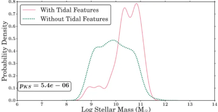
pKS= 5.4e−06
With Tidal Features Without Tidal Features
Figure 13. Distributions of stellar mass for gas-poor galaxies with (pink) and without (teal) tidal features. The gas-poor galaxies with tidal features are more massive than their counterparts without tidal features at∼4.5σsignificance. These kernel density estima-tions were created with a Gaussian kernel and a cross-validated optimal bandwidth of 0.29 dex.
isons of the µ∆ versus G/S ratio distributions for gas-rich galaxies with and without tidal features are shown in Figure10; the same distributions for gas-poor galaxies are shown in Figure11. According to Figure10, gas-rich galaxies with tidal features tend to be less bulged than their counterparts without tidal features as they increase in G/S ratio at a significance of pP F F ∼10−9; in con-trast, there is not a significant difference between the distributions ofµ∆v. G/S for gas-poor galaxies. Again, these results point to different origins for tidal features depending on gas fraction.
3.6. Stellar Mass
According to the Random Forest analysis in Section 3.3, stellar mass is the 5th most important feature for predicting the presence of tidal features, but we discuss it before the 4th (nearest neighbor distance) for simplic-ity. The stellar mass distributions for our gas-rich and gas-poor galaxies are shown in Figures 12 and 13, re-spectively. Though gas-rich galaxies with tidal features appear to have a slightly bimodal distribution, the differ-ence compared to gas-rich galaxies without tidal features is not weakly significant. In contrast, gas-poor galaxies show a much more prominent relationship between tidal features and stellar mass, with a ∼4.5σ significant dif-ference between the M∗ distributions for galaxies with and without tidal features. Darg et al. (2010) similarly
found no difference in the stellar masses of spiral galaxies with tidal features, in contrast to a marked increase in stellar mass for elliptical galaxies in mergers versus their control counterparts. Assuming their elliptical galaxies are mostly gas-poor, these results are compatible with our findings.
3.7. Environment
To analyze the environments of our galaxies, we consid-ered both nearest neighbor distance and group mass and richness to consider environmental influences on both the local and halo scale.
3.7.1. Nearest Neighbor Distance
For each galaxy in RESOLVE, we have calculated the projected distance to its nearest neighbor using the kd-tree algorithm described in Section 2.1.4 and removing peculiar velocities. We compare the distributions of pro-jected distances for galaxies with and without tidal fea-tures within our gas-rich and gas-poor subsamples in
Fig-ures 14a and 15a, respectively. In panels b and c, we
further divide each subsample based on whether the near-est neighbor is a member of the same group. The Mann-Whitney-U (MWU) test has been applied to each pair of distributions in addition to the K-S test. Both the MWU and K-S tests return p-values that test the null hypothe-sis that the two samples have the same distribution. One difference is that the MWU test is mainly sensitive to dis-crepancies between the two medians while the K-S test is more sensitive to general differences between the two distributions (shape, spread, median, etc.). Another dif-ference is that the K-S test is not suited for samples with ties. Since we expect pairs of duplicate nearest-neighbor distances, the MWU test may provide a more accurate p-value.
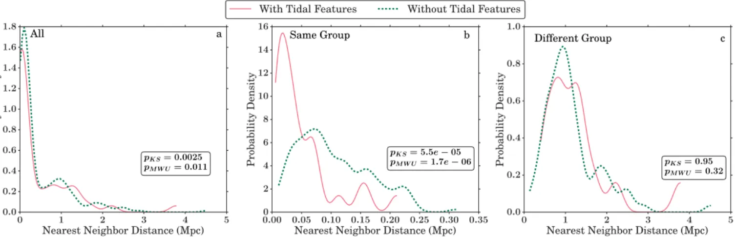
For gas-rich galaxies with neighbors in the same group, those with/without tidal features have a median sepa-ration of 0.06/0.1 Mpc; the difference between the two distributions is significant at a ∼ 3σ level. Similarly, for gas-poor galaxies with neighbors in the same group, those with/without tidal features have a median sepa-ration of 0.03/0.09 Mpc; the difference between the two distributions is significant at a∼4.5σlevel. However, re-gardless of gas content, galaxies with neighbors outside of their own group do not show a correlation between the presence of tidal features and nearest neighbor distance. We obtain results similar to these kd-tree results if we instead calculate nearest neighbor distances as projected distances to the nearest neighbor in a cylindrical volume within cz = 500 km/s of the main object.
Thus, regardless of gas content, we find that galaxies with neighbors in the same group are closer to their near-est neighbors if they have tidal features than if they do not, with a stronger result observed for gas-poor galaxies than gas-rich ones. We infer that a large fraction of de-tected tidal features are a result of ongoing interactions, or early-stage mergers, especially in gas-poor galaxies.
3.7.2. Group Mass and Richness
nearest-0 2 4 6 8 10 Nearest Neighbor Distance (Mpc) 0.0
0.1 0.2 0.3 0.4 0.5 0.6 0.7 0.8
Probability
Density
pKS= 0.083 pM W U= 0.19
All a
0.0 0.1 0.2 0.3 0.4 0.5 Nearest Neighbor Distance (Mpc) 0
1 2 3 4 5 6 7 8 9
Probability
Density
pKS= 0.0027 pM W U= 0.0012
Same Group b
With Tidal Features Without Tidal Features
0 2 4 6 8 10
Nearest Neighbor Distance (Mpc) 0.0
0.1 0.2 0.3 0.4 0.5 0.6 0.7
Probability
Density
pKS= 0.49 pM W U= 0.28
Different Group c
Figure 14. Distributions of nearest neighbor distances for gas-rich galaxies with (blue) and without (orange) tidal features. Panel (a) shows the two distributions, whose difference is not statistically-significant. These populations are further divided into galaxies whose nearest neighbors are within the same groups (b) and galaxies with neighbors outside of their groups (c). The gas-rich galaxies with tidal features and neighbors within their group are closer to their nearest neighbors than their counterparts without tidal features at a∼3σ significance. Gas-rich galaxies with nearest neighbors outside of their group do not show a similarly significant result. These kernel density estimations were created with a Gaussian kernel and a cross-validated optimal bandwidth of 0.20 Mpc.
0 1 2 3 4 5
Nearest Neighbor Distance (Mpc)
0.0
0.2
0.4
0.6
0.8
1.0
1.2
1.4
1.6
1.8
Probability
Density
pKS= 0.0025
pM W U= 0.011
All a
0.00 0.05 0.10 0.15 0.20 0.25 0.30 0.35
Nearest Neighbor Distance (Mpc) 0
2 4 6 8 10 12 14 16
Probability
Density
pKS= 5.5e−05
pM W U= 1.7e−06
Same Group b
With Tidal Features Without Tidal Features
0 1 2 3 4 5
Nearest Neighbor Distance (Mpc)
0.0
0.2
0.4
0.6
0.8
1.0
Probability
Density
pKS= 0.95
pM W U= 0.32
Different Group c
Figure 15. Distributions of nearest neighbor distances for gas-poor galaxies with (pink) and without (teal) tidal features. Panel (a) shows the two distributions; those with tidal features appear to be closer to their nearest neighbors at around a∼2σsignificance. These populations are further divided into galaxies whose nearest neighbors are within the same groups (b) and galaxies with neighbors outside of their groups (c). The gas-poor galaxies with tidal features and neighbors within their group are closer to their nearest neighbors than their counterparts without tidal features at a∼4.5σ significance. Gas-poor galaxies with nearest neighbors outside of their group do not show a similarly significant result. These kernel density estimations were created with a Gaussian kernel and a cross-validated optimal bandwidth of 0.20 Mpc.
neighbor distance shown in Figure 15 implies an en-vironmental dependence for our gas-poor sample. The distributions of the group halo mass for our gas-rich and gas-poor subsamples with each subdivided into galaxies with and without tidal features are shown in Figures 16
and 17, respectively. Though we do not find a
statis-tically significant difference between the halo masses of gas-rich galaxies with and without tidal features, halo masses of gas-poor galaxies with tidal features appear to be marginally more massive than for their counterparts without tidal features at a∼2.5σsignificance.
However, considering not only the mass of the group halo, but also the number of galaxies within the group, we find a trend in the relationship of group number ver-sus group halo mass for gas-poor galaxies (Figure 18). At a fixed group halo mass, gas-poor galaxies with tidal
9 10 11 12 13 14 15
Log Group Halo Mass (M)
0.0 0.2 0.4 0.6 0.8 1.0 1.2
Probability
Density
pKS= 0.36 pM W U= 0.076
With Tidal Features Without Tidal Features
Figure 16. Distributions of the group halo masses of gas-rich galaxies with (green) and without (purple) tidal features. We do not find a statistically-significant difference between the two dis-tributions. These kernel density estimations were created with a Gaussian kernel and a cross-validated optimal bandwidth of 0.13 dex.
10 11 12 13 14 15 16 17
Log Group Halo Mass (M)
0.0
0.1
0.2
0.3
0.4
0.5
0.6
0.7
Probability
Density
pKS= 0.0015 pM W U= 0.0014 With Tidal Features Without Tidal Features
Figure 17. Distributions of the group halo masses of gas-poor galaxies with (green) and without (purple) tidal features. The gas-poor galaxies with tidal features tend to reside in larger group halos with a ∼3σ significance. These kernel density estimations were created with a Gaussian kernel and a cross-validated optimal bandwidth of 0.21 dex.
10.5 11.0 11.5 12.0 12.5 13.0 13.5 14.0
Log Group Halo Mass (M) 0
5 10 15 20 25 30 35 40
Number
of
Galaxies
in
Group
pP F F= 0.021 Gas-Poor Galaxies with Tidal Features
0.01 0.02 0.03 0.04 0.05 0.06 0.07 0.08
Density of Gas-Poor Galaxies without Tidal Features
Figure 18. Number of group members versus group halo mass for our gas-poor sample. The overall number of gas-poor galaxies without tidal features in each hexbin is shown by the color bar, while those with tidal features are overplotted in blue.
have tidal features, although we do see a difference in nearest neighbor distance.
4. DISCUSSION
Although we discussed the effects of surface brightness limitations in section 3.1, other detection biases affect our ability to detect tidal features. Principally, the time-scale over which a feature is detectable depends on the internal properties of the progenitor (Darg et al. 2009). Simulations of equal-mass gas-rich mergers show time-scales depend strongly on geometric parameters like the pericentric distance and relative orientation of the galax-ies (Lotz et al. 2008). In addition, gas fraction correlates strongly with tidal feature longevity; Lotz et al. (2010) found that asymmetry was detectable from ≤ 300 Myr for fgas∼20% to≥1 Gyr for fgas∼50%. Thus, galaxies we classified as lacking tidal features may have had re-cent mergers or interactions >300 Myr ago but appear relaxed. This effect is especially pronounced for gas-poor galaxies, possibly explaining the overall increase in gas-to-stellar-mass ratio seen in our tidal feature population in Figure4.
Due to this difference in observability, studying gas-rich and gas-poor galaxies separately helps restrict our analyses to galaxies with similar feature time-scales. We studied the relationship between the presence of tidal features and other progenitor properties such as mor-phology, star formation history, stellar mass, and envi-ronment. Only our gas-rich galaxies showed strong re-sults when looking at the morphology metric µ∆as well as star formation history as shown in Figures 6, 8, and 10. In contrast, only the gas-poor galaxies with tidal fea-tures had significantly-different stellar masses and group haloes. Both gas-rich and gas-poor galaxies with nearest neighbors in their group and tidal features were closer to these neighbors than their counterparts without tidal features.
mass scale at which cold-mode accretion is expected to dominate (Kere˘s et al. 2009). This scale also corresponds to the ”gas-richness threshold scale” (Kannappan et al. 2013) below which gas-rich galaxies are the norm. Fu-ture work on the satellite populations of our galaxies with tidal features could solidify our environmental analyses while allowing us to further probe the effect of interac-tions with small neighbors. While we cannot definitively point to a single origin scenario for the tidal features around our gas-rich galaxies, gas accretion could create many of these morphological disturbances. Thus, tidal features around gas-rich galaxies may arise from gas ac-cretion, mergers, or some from a combination of the two. Future analysis of the star-formation histories and mor-phologies of gas-rich galaxies with close neighbors versus those with neighbors in other groups could help separate these populations by their evolutionary history.
In contrast, our subsample of gas-poor galaxies with tidal features does not show increased gas-to-stellar-mass ratios nor elevated star formation as one might expect from an accretion event. However, they do appear to be closer to their nearest neighbor than their counterparts without tidal features. Thus, these tidal features could result from ongoing interactions with these neighbors. Furthermore, the gas-poor galaxies with tidal features also reside in groups with fewer members at a fixed halo mass, which could imply a substantial fraction of merger remnants in this sample. When two galaxies merge, the group halo mass would remain the same while the num-ber of memnum-bers decreased. However, our study of the number of group members versus halo mass yields only tentative results that would benefit from a larger sample size of gas-poor galaxies. In addition, gas-poor galaxies with tidal features have much higher stellar masses than those without; in fact, low-mass, gas-poor galaxies lack tidal features detected in this study. This trend could be consistent with a large number of central galaxies among our poor giants as well as a larger number of gas-poor dwarf satellites. Low-mass, gas-gas-poor galaxies are mainly satellites, which move too quickly in their orbits around the central to merge. Thus, only satellites closely approaching their central galaxies would show signs of tidal features. In contrast, centrals remain relatively stationary, allowing for accretion of both gas and com-panion satellite and thus the formation of tidal features. However, central status was one of the least important features in our Random Forest analysis in Section 3.3. Performing a separate Random Forest analysis of solely gas-poor galaxies may provide better insight into the rel-ative importance of central/satellite status. Overall, dry interactions and mergers appear to be the driving cause of tidal features around our gas-poor galaxies. However, Lotz et al. (2010) found that at high gas fractions, asym-metry is equally likely to indicate major and minor merg-ers, but at low and moderate gas fractions asymmetry mainly indicates major mergers. Thus, we may be less able to identify signs of minor mergers within our gas-poor population, creating a false perception of evolution-ary histories dominated by major mergers.
5. CONCLUSIONS
In this work, we have performed a census of tidal fea-tures around galaxies in the REsolved Spectroscopy of a Local VolumE (RESOLVE) survey using images from
DECaLS. Of the 1027 RESOLVE galaxies visually in-spected for tidal features, 21±2% of the galaxies show faint substructure in the DECaLS images. However, due to limitations of survey depth and background uncer-tainty, this percentage should be seen as a lower limit of the occurrence of these features.
We have used this sample to study the relationship between gas content, structure, star formation history, morphology, stellar mass, galaxy environment, and the detection of tidal features. Our key results are as follows.
1. We find that galaxies with tidal features tend to have higher gas-to-stellar-mass ratios (G/S) than those without. This correlation is particularly sig-nificant for galaxies with log(G/S)>-1.
2. We observe elevated short- and long-term star formation rates, less-bulged morphologies, and shorter distances to nearest neighbors (when the neighbor is in the same group as the galaxy) for gas-rich galaxies with tidal features than are seen for galaxies without tidal features. We do not find any statistically significant differences between the stellar and halo mass distributions of our gas-rich galaxies with and without tidal features.
3. In contrast, gas-poor galaxies with tidal features do not show significantly different G/S ratios, star formation histories, and morphologies in compari-son to gas-poor galaxies without tidal features. In-stead, galaxies with tidal features in this subsample have higher stellar masses, closer distances to their nearest-neighbor (if the neighbor is in the same group), and larger halo masses. We also observe a weak indication that gas-poor galaxies with tidal features reside in groups with fewer members at a fixed halo mass than those without tidal features.
These results lend support to different origin scenarios for tidal features around gas-rich and gas-poor galaxies. While the nearest-neighbor result for gas-rich galaxies is most likely driven by interactions, the stronger results related to gas content, star formation, and morphology point towards other causes, i.e. gas accretion or accre-tion of small neighbors. Gas-poor galaxies with tidal features show stronger environmental differences when compared to those without, pointing to dry interactions and mergers as the main origin scenarios for tidal fea-tures in this subsample. We next turn to further study of these subsamples with other environmental parameters, particularly a study of potential small neighbors below the completeness limit of RESOLVE, role in the group environment (i.e. central versus satellite), and location of neighbor galaxies (i.e. within or outside of the group) in order to continue studying the evolutionary origins of these tidal features in the nearby universe.
ACKNOWLEDGMENTS
addition, I would like to thank Alexie Leauthaud and the CS82 team for data access that helped launch this work, even though the data was not ultimately used. This work was supported a North Carolina Space Grant Undergrad-uate Research Scholarship. RESOLVE is funded by NSF CAREER award 0955368. This research uses services or data provided by the Science Data Archive at NOAO. NOAO is operated by the Association of Universities for Research in Astronomy (AURA), Inc. under a coopera-tive agreement with the National Science Foundation.
Funding for SDSS-III has been provided by the Al-fred P. Sloan Foundation, the Participating Institutions, the National Science Foundation and the US Depart-ment of Energy Office of Science. The SDSS-III web site is http://www.sdss3.org/. SDSS-III is managed by the Astrophysical Research Consortium for the Partici-pating Institutions of the SDSS-III Collaboration includ-ing the University of Arizona, the Brazilian Participa-tion Group, Brookhaven NaParticipa-tional Laboratory, sity of Cambridge, Carnegie Mellon University, Univer-sity of Florida, the French Participation Group, the Ger-man Participation Group, Harvard University, the Insti-tuto de Astrofsica de Canarias, the Michigan State/Notre Dame/JINA Participation Group, Johns Hopkins Uni-versity, Lawrence Berkeley National Laboratory, Max Planck Institute for Astrophysics, Max Planck Insti-tute for Extraterrestrial Physics, New Mexico State Uni-versity, New York UniUni-versity, Ohio State UniUni-versity, Pennsylvania State University, University of Portsmouth, Princeton University, the Spanish Participation Group, University of Tokyo, University of Utah, Vanderbilt Uni-versity, University of Virginia, University of Washington and Yale University
REFERENCES
Adams S. M., Zaritsky D., Sand D. J., Graham M. L., Bildfell C., Hoekstra H., Pritchet C., 2012, AJ, 144, 128
Abraham, R.G., Tanvir, N.R., Santiago, B.X., Ellis, R.S., Glazebrook, K., van den Bergh, S.: MNRAS 279, L47 (1996)
Aihara, H., Allende Prieto, C., An, D., et al. 2011, ApJS, 193, 29
Battaglia N. et al., 2015, arXiv:1509.08930
Berlind, A. A., Frieman, J., Weinberg, D. H., et al. 2006, ApJS, 167, 1
Bertin, E. and Arnouts, S. 1996, A&AS, 117, 393 Bournaud, F., et al. 2011, ApJ, 730, 4
Bridge, C., Carlberg, R.G., & Sullivan M. 2010, ApJ, 709, 1067
Breiman, L. Machine Learning (2001) 45: 5. doi:10.1023/A:1010933404324
Bullock, J. S. and Johnston, K. V. 2005, ApJ, 635, 931 Colless, M., Dalton, G., Maddox, S., et al. 2001,
MN-RAS, 328, 1039
Conselice, C.J., Rajgor, S., Myers, R. 2008, MNRAS, 386, 909
DOnghia E., Vogelsberger M., Faucher-Giguere C.-A., Hernquist L., 2010, ApJ, 725, 353
Darg D. W., et al., 2010, MNRAS, 401, 1552
Driver, S. P., Hill, D. T., Kelvin, L. S., et al. 2011, MNRAS, 413, 971
Duarte, M., & Mamon, G. A. 2014, MNRAS, 440, 1763 Duc P.-A., Renaud F., 2013, in Souchay J., Mathis
S., Tokieda T., eds, Lecture Notes in Physics, Vol. 861, Tides in Astronomy and Astrophysics. Springer-Verlag, Berlin, p. 327
Duc, P.-A., Cuillandre, J.-C., Karabal, E., et al., 2015, Monthly Notices of the Royal Astronomical Society, 446, 120
Eckert, K., Kannappan, S. J., Stark , D. V., et al. 2015, ApJ, 810, 166
Ebrova, I. 2013, ArXiv e-prints
Eckert, K., Kannappan, S. J., Stark, D. V., et al. 2015, ApJ, 810, 166
Eckert, K. D., Kannappan, S. J., Stark, D. V., et al. 2016, ApJ, 824, 124
Ellison, S. L., Fertig, D., Rosenberg, J. L., Nair, P., Simard, L., Torrey, P., Patton, D. R., 2015, MNRAS, 448, 221
Erben, T., Kneib, J.-P., Leauthaud, A., et al., in prepa-ration
Falco, E. E., Kurtz, M. J., Geller, M. J., et al. 1999, PASP, 111, 438
Fasano, G., & Franceschini, A. 1987, MNRAS, 225, 155
Fliri, J., & Trujillo, I. 2016, MNRAS, 456, 1359 Geisser, S., 1975, The predictive sample reuse method
with applications. J. Amer. Statist. Assoc., 70:320328.
Griffiths, R.E., Casertano, S., Ratnatunga, K.U., Neuschaefer, L.W., Ellis, R.S., et al.: ApJ, 435, L19 (1994)
Hambly, N. C., Collins, R. S., Cross, N. J. G., et al. 2008, MNRAS, 384, 637
Haynes, M. P., Giovanelli, R., Martin, A. M., et al. 2011, AJ, 142, 170
Hopkins, P. F., Cox, T. J., Younger, J. D., & Hern-quist, L. 2009, ApJ, 691, 1168
Hopkins, P. F., et al. 2009, MNRAS, 397, 802
Ji, I., Peirani, S., & Yi, S. K. 2014, Astronomy & As-trophysics, 566, A97
Jones, D. H., Read, M. A., Saunders, W., et al. 2009, MNRAS, 399, 683
Joye, W. A. and Mandel, E. 2003, ASPC, 295, 489 Kannappan, S. J., & Gawiser, E. 2007, ApJ, 657, L5 Kannappan, S. J., & Wei, L. H. 2008, in AIP Conf.
Ser. 1035, The Evolution of Galaxies Through the Neutral Hydrogen Window, ed. R. Minchin & E. Momjian (Melville, NY: AIP), 163
Kannappan, S. J., Stark, D. V., Eckert, K. D., et al. 2013, ApJ, 777, 42
Landis, J., & Koch, G. (1977). The Measurement of Observer Agreement for Categorical Data. Biomet-rics, 33(1), 159-174. doi:10.2307/2529310
Lisenfeld U. et al., 2011, A&A, 534, A102
Lotz, J. M., Jonsson, P., Cox, T. J., & Primack, J. R. 2008, MNRAS, 3 91, 1137
Lotz, J. M., Jonsson P., Cox T. J., Primack J. R., 2010, MNRAS, 404, 590
Lotz, J. M., Jonsson, P., Cox, T. J., Croton, D., Pri-mak, J. R., Somerville, R. S., & Stewart, K. 2011, The Astrophysial Journal, 742, 103
Maneewongvatana S., Mount D. M., 1999, eprint arXiv:cs/9901013
Miskolczi, A., Bomans, D. and Dettmar, R. 2011,A&A, 536, 66
2015, ApJ, 812, 89
Morrissey, P., Conrow, T., Barlow, T. A., et al. 2007, ApJS, 173, 682
Moster, B.P., Macci`o, A.V., Somerville, R.S., et al. 2011, MNRAS, 415, 3750
Naab, T., Jesseit, R., Burkert, A. 2006, MNRAS, 372, 839
Paturel, G., Petit, C., Prugniel, P., et al. 2003, A&A, 412, 45
Peacock, J. A. 1983, MNRAS, 202, 615
Pedregosa, F., Varoquaux, G., Gramfort, A., et al. 2011, Journal of Machine Learning Research, 12, 2825
Perez, J., Michel-Dansac, L., & Tissera, P. B. 2011, MNRAS, 417, 580
Perret, V., Renaud, F., Epinat, B., Amram, P., Bour-naud, F., Contini, T., Teyssier, R., & Lambert, J.-C. 2014, A&A, 562, A1
Rafieferantsoa, M., Dav e, R., Angl es-Alcazar, D., et al. 2014, A rXiv e-prints, arXiv:1408.2531
Richer, M. G., Georgiev, L., Rosado, M., Bullejos, A., Valdez-Gutierrez, M., & Dultzin-Hacyan, D. 2003, A&A, 397, 99
Roming, P. W. A., Kennedy, T. E., Mason, K. O., et al. 2005, SSRv, 120, 95
Sales L. V., Navarro J. F., Theuns T., Schaye J., White S. D. M., Frenk C. S., Crain R. A., Dalla Vecchia C., 2012, MNRAS, 423, 1544
Schlegel, D. J., Blum, R. D., Castander, F. J., et al. 2015, in American Astronomical Society Meeting Ab-stracts, Vol. 225, American Astronomical Society Meeting Abstracts, 336.07
Scudder J. M., Ellison S. L., Momjian E., Rosenberg J. L., Torrey P., Patton D. R., Fertig D., Mendel J. T., 2015, MNRAS, 449, 3719
Skrutskie, M. F., Cutri, R. M., Stiening, R., et al. 2006, AJ, 131, 1163
Stark, D. V., Kannappan, S. J., Wei, L. H., et al. 2013, ApJ, 769, 82
Stark, D. V., Kannappan, S. J., Eckert, K. D., et al., 2016, ApJ, 832, 126
Stewart, K. R., Kaufmann, T., Bullock, J. S., et al. 2011, ApJ, 738, 39
Tonnesen, S., & Cen, R. 2012, MNRAS, 425, 2313 Toomre, A., & Toomre, J. 1972, ApJ, 178, 623 van Dokkum, P. 2005, AJ, 130, 2647
APPENDIX
Figure 19. Original DECaLS image as well as the masked image of rf0138. A stellar stream is clearly visible coming out of the left side of the galaxy.
Figure 20. Original DECaLS image as well as the masked image of rs0112. This galaxy hosts a stellar stream which loops around the upper left of the image then crosses to the lower left.