ABSTRACT
Ozone is a powerful oxidant used in the water-treatment industry to make drinking water wholesome and to remove undesirable taste, odor and color. In order to evaluate such treatment processes, it is imperative to understand the decomposition
kinetics of aqueous ozone. The decomposition of aqueous ozone occurs via chain reactions involving hydroxyl radicals. Many dissolved substances in water react with the hydroxyl radicals and alter the rate of aqueous ozone decomposition. This study examines the effects of pH, carbonate and humic substances on aqueous ozone decomposition. Batch kinetic experiments were conducted at 22 "C in solutions containing 0.01 M total phosphate species and total
carbonate species concentration varying from 0 to 10 x 10'' M. The
experimental data suggest that ozone decomposition in the presence of carbonate species conforms to simple first-order kinetics. The rate of ozone decomposition increased with increase in pH and was retarded with increase in carbonate species concentration, due to scavenging of the hydroxyl radicals. Ozone decomposition in thepresence of humic substances was characterized by an initial immediate rapid ozone utilization followed by first-order depletion
of ozone. Similar behavior was observed in natural waters. The
pseudo-first-order rate constants decreased with increase in
initial ozone dose and decreased with increase in initial concentration of humic material. The Staehelin and Hoigne (1985)
involved during ozone depletion. A correlation reported in the
ACKNOWLEDGEMENTS
This project was funded by the American Water Works
Association Research Foundation.
I would like to thank my advisor, Dr. Philip Singer for
the contribution of his patient support and expertise. I also owe thanks to Mr. Chris Hull for all his ideas and assistance.
Additional thanks to Dr. Mark Sobsey and his group of students for their help in the form of computer time and facilities.
Mr. Richard Hall's assistance with the fabrication of the
experimental set-up is greatly appreciated. I also extend my thanks to Mr. Tony Greiner for helping me with the analysis of
natural water samples.
Most of all, I thank my parents, for their encouragement
TABLE OF CONTENTS
Page
List of Tables... vi
List of Figures... ix
1. Introduction ... 1
2. Theoretical Background ... 5
A. Aqueous Ozone Decomposition ... 5
(i) Effect of pH and Temperature... 5
(ii) Effect of Humic Material... 13
B. Kinetic Models for Ozone Decomposition .... 17
(i) Ozone Decomposition in Pure Water ... 17
(ii) Aqueous Ozone Decomposition in the Presence of Humic Material ... 19
3. Experimental Methods ... 23
A. Introduction... 23
B. Experimental Set-up... 23
C. Experimental Procedure ... 27
(i) Initial Preparation ... 27
(ii) Test Solution Preparation and Sampling Methods ... 29
D. Analytical Procedures for Aqueous Ozone Measurement... 32
(i) lodometric Method... 32
(ii) UV Method... 33
Page
4. Results and Discussion... 41
A. Introduction... 41
B. Effect of pH ... . ... .... 41
C. Effect of Carbonate and Bicarbonate Ions ... 56
D. Effect of Hvunic Material... 72
E. Ozone Depletion in Natural Waters ... 94
F. Engineering Applications of Results ... 102
5. Conclusions... 104
6. References... 107
7. Appendices ... 112
Appendix A Effect of Quality of Buffer
Chemicals on Ozone Decomposition 112
Appendix B Derivation of the Mixed-Order Rate
Equation Using the Staehelin and Hoigne
Mechanism 114
Appendix C Derivation of the Generalized Mixed-Order
Rate Equation Using the Staehelin and
Hoigne Mechanism 117 Appendix D Data Analysis Procedures and Sample
Calculations 120 Appendix E
Appendix F
Derivation of the Rate Equation for Ozone
Depletion in the Presence of Humic
Substances Using the Staehelin and Hoigne
Mechanism 128
Results of Selected Experiments on Dis¬
Table 2. 1
Table 2. 2
Table 2 3 Table 2 .4
Table 3 .1
Table 4 .1
Table 4 .2
Table 4 .3
Table 4.4
Table 4 .5
Table 4 .6
Table 4 .7
Table 4 .8
Table 4 9
Table 4. 1
List of Tables
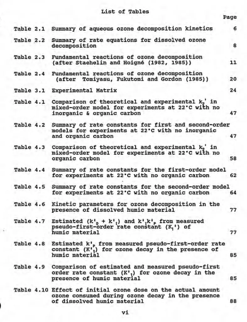
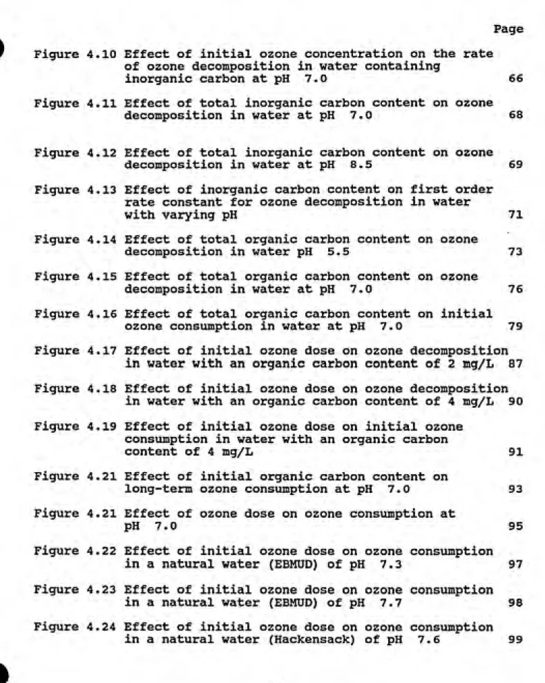
Summary of aqueous ozone decomposition kinetics Summary of rate equations for dissolved ozone decomposition
Fundamental reactions of ozone decomposition (after Staehelin and Hoigne (1982, 1985)) Fundamental reactions of ozone decomposition
(after Tomiyasu, Fukutomi and Gordon (1985))
Experimental Matrix
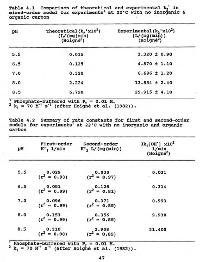
Comparison of theoretical and experimental k,' in
mixed-order model for experiments at 22'C with no inorganic & organic carbon
Page 6 8 11 20 24 47 Summary of rate constants for first and second-order models for experiments at 22"C with no inorganic
and organic carbon 47
Comparison of theoretical and experimental k,' in
mixed-order model for experiments at 22°C with no
organic carbon 58
Summary of rate constants for the first-order model for experiments at 22"C with no organic carbon 62 Summary of rate constants for the second-order model for experiments at 22'C with no organic carbon 64
Kinetic parameters for ozone decomposition in the
presence of dissolved humic material 77
Estimated (k'p + k',) and k',k'p from measured
pseudo-first-order rate constant (K,') of
humic material 77
Estimated k'p from measured pseudo-first-order rate
constant (K*^) for ozone decay in the presence of
humic material 85 Comparison of estimated and measured pseudo-first
order rate constant (K',) for ozone decay in the
presence of humic material 85 10 Effect of initial ozone dose on the actual amount
ozone consumed during ozone decay in the presence
Page
Table 4.11 Effect of initial ozone dose on the kinetic
parameters for ozone decomposition in the presence
of dissolved humic material 88 Table 4.12 Effect of initial ozone dose on the kinetic
parameters for ozone consumption in natural waters 101
Table 4.13 Comparison of estimated and measured pseudo-first
order rate constant (K'^) for ozone consumption in
natural waters 101
Table B.l Fundamental reactions of dissolved ozone
decomposition (after Staehelin and Hoigne
(1982,1985)) 114
Table C.l Reactions of dissolved substances with ozone and
hydroxide radical formed during ozone decomposition 117
Table D.l Experimental k'g values for experiments conducted
at 22'C, pH 5.5 with 0.01 M total phosphate and no
inorganic & organic carbon 123
Table D.2 Equilibrium constant correction factor for ionic
strength effects. (Using Equation (B.IO)) 123
Table D.3 Theoretical k'g values for experiments conducted
at 22''C, pH 5.5 with 0.01 M total phosphate and no
organic carbon 123
Table D.4 Experimental k'j values for experiments conducted
at 22°C, pH 5.5 with 0.01 M total phosphate and
0.002 M total carbonate and no organic carbon 126
Table D.5 Dissociation fractions of phosphoric acid at
relevant pH values at 22 "C with /i = 0.01 127
Table D.6 Dissociation fractions of carbonic acid at
relevant pH values at 22 "C with /x = 0.01
in water 127 Table E.l Reactions of dissolved humic substances with ozone
and hydroxide radical formed during ozone decomposi¬
tion in water 128 Table F.l Residual ozone concentration versus time data
illustrating the effect of pH on ozone decomposi¬
tion experiments conducted at 22°C with no
Page Table F.2 Residual ozone concentration versus time data
illustrating the effect of pH on ozone decomposi¬
tion in experiments conducted at 22"C with
0.002 M C^ and no organic carbon 134
Table F.3 Residual ozone concentration versus time data
illustrating the effect of C^ on ozone decomposi¬
tion in experiments conducted at 22'C and pH 7.0
with no organic carbon 134 Table F.4 Residual ozone concentration versus time data
illustrating the effect of Cj, on ozone decomposi¬
tion in experiments conducted at 22°C and pH 7.0
with no organic carbon 135
Table F.5 Residual ozone concentration versus time data illustrating the effect of humic acid content on ozone depletion in experiments conducted at 22°C
and pH 5.5 with 0.002 M C^ ' 135
Table F.6 Residual ozone concentration versus time data
illustrating the effect of humic acid content on ozone depletion in experiments conducted at 22'C
and pH 7.0 with 0.002 M C^ 136
Table F.7 Residual ozone concentration versus time data
illustrating the effect of C^ on ozone depletion
in experiments conducted at 22"C and pH 7.0 with
0.002 M C^ 137 Table F.8 Residual ozone concentration versus time data
illustrating the effect of C^ on ozone depletion
in EBMUD water at 18"C and pH 7.6 with 3.90 mg/LTOC and alkalinity 60 mg/L 137
Table F.9 Residual ozone concentration versus time data
illustrating the effect of C^ on ozone depletion
Figure 2.1 Figure 2.2 Figure 3.1 Figure 3.2 Figure 3.3 Figure 3.4 Figure 3.5 Figure 4.1 Figure 4.2 Figure 4.3 Figure 4.4 Figure 4.5 Figure 4.6 Figure 4.7 Figure 4.8 Figure 4.9
List of Figures
Reactions of dissolved ozone in pure water (after Staehelin and Hoigne, 1982)
Reactions of dissolved ozone with humic material
(after Feng and Legube, 1991) Schematic of Experimental Set-up
Schematic of Experimental Batch Reactor Calibration Curve I of indigo method for 0-6 mg/L dissolved ozone
Calibration Curve II of indigo method for
0-3 mg/L dissolved ozone
Calibration Curve III of indigo method for 0-1 mg/L dissolved ozone
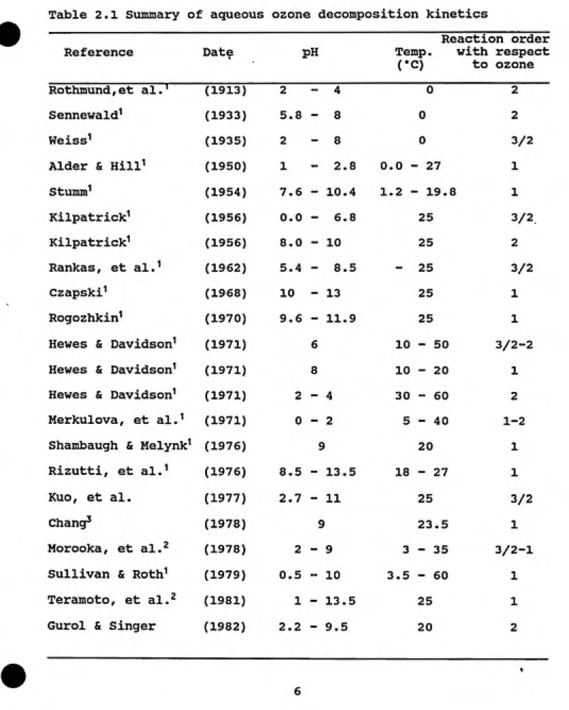
Page 10 14 26 28 38 39 40 Decomposition of ozone in water at pH 2.0,
demonstrating no ozone loss due to volatilization 42
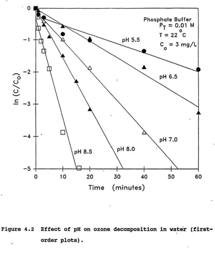
Effect of pH on ozone decomposition in water
(first-order plots) 50
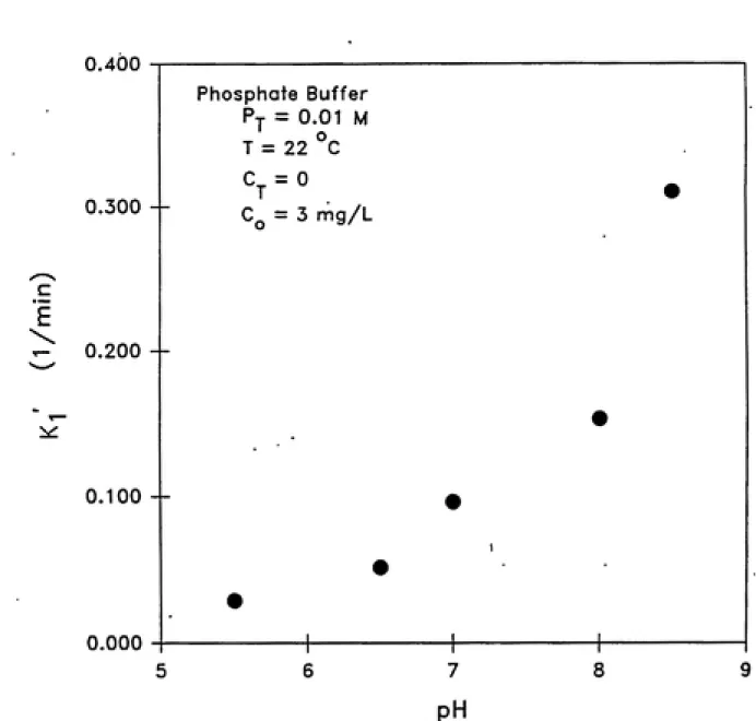
Effect of pH on first order rate constant of ozone
decomposition in water 52
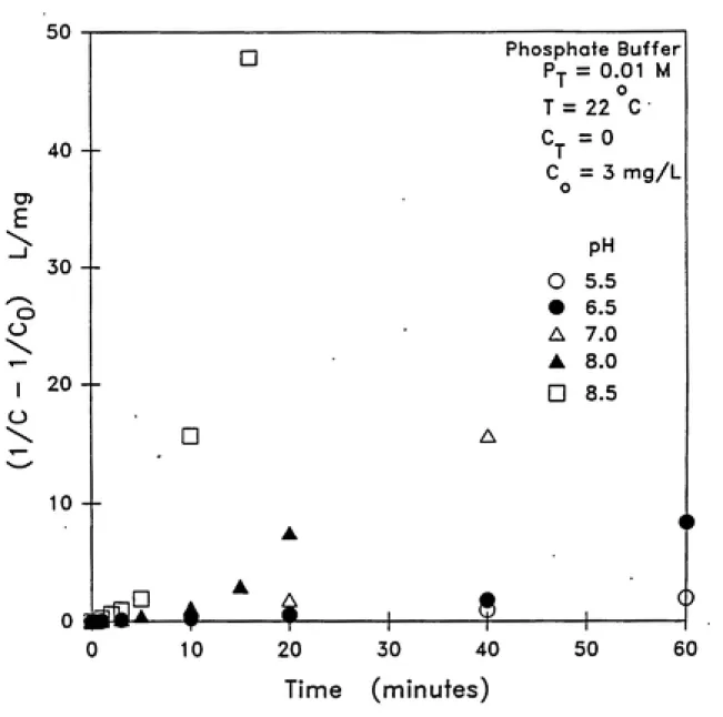
Effect of pH on ozone decomposition in water
(second-order plots) 53 Comparison of first and second-order models to
describe ozone decomposition in water 54
Effect of initial ozone dose on the rate of ozone
decomposition in water at pH 7.0 55
Effect of pH on ozone decomposition in water
containing 0.002 M total inorganic carbon
(first-order plots) 59 Effect of pH on ozone decomposition in water
containing 0.002 M total inorganic carbon (second-order plots) 60 Comparison of first and second-order models to
Page Figure 4.10 Effect of initial ozone concentration on the rate
of ozone decomposition in water containing
inorganic carbon at pH 7.0 66
Figure 4.11 Effect of total inorganic carbon content on ozone
decomposition in water at pH 7.0 68
Figure 4.12 Effect of total inorganic carbon content on ozone
decomposition in water at pH 8.5 69
Figure 4.13 Effect of inorganic carbon content on first order
rate constant for ozone decomposition in water
with varying pH 71 Figure 4.14 Effect of total organic carbon content on ozone
decomposition in water pH 5.5 73 Figure 4.15 Effect of total organic carbon content on ozone
decomposition in water at pH 7.0 76 Figure 4.16 Effect of total organic carbon content on initial
ozone consumption in water at pH 7.0 79 Figure 4.17 Effect of initial ozone dose on ozone decomposition
in water with an organic carbon content of 2 mg/L 87
Figure 4.18 Effect of initial ozone dose on ozone decomposition
in water with an organic carbon content of 4 mg/L 90 Figure 4.19 Effect of initial ozone dose on initial ozone
consumption in water with an organic carbon
content of 4 mg/L 91 Figure 4.21 Effect of initial organic carbon content on
long-term ozone consumption at pH 7.0 93
Figure 4.21 Effect of ozone dose on ozone consumption at
pH 7.0 95
Figure 4.22 Effect of initial ozone dose on ozone constimption in a natural water (EBMUD) of pH 7.3 97 Figure 4.23 Effect of initial ozone dose on ozone consumption
in a natural water (EBMUD) of pH 7.7 98 Figure 4.24 Effect of initial ozone dose on ozone consumption
Page
Figure A.l Effect of quality of buffer chemicals on ozone
decomposition in water at pH 7.0 113
Figure D.l Variation of experimenatal kg' with time
in experiments conducted at pH 8.5 122 Figure E.l Reactions of dissolved ozone in the presence of
solute HA which react with ozone or which interact
with hydroxyl (OH) radicals by scavenging and/or converting OH into HOg (after Staehelin and
1. INTRODUCTION
The main purpose of drinking water treatment is to make
the water safe to drink. Outbreaks of waterborne diseases such as
typhoid, cholera, hepatitis etc. were widespread until water
treatment came into being approximately a century ago. Chlorine
has been the most common disinfectant used to quell the outbreaks
of such waterborne diseases.
Over the last two decades, there has been growing concern
about the interactions between chlorine and naturally-occurring
organic matter in raw water to produce by-products which are
suspected carcinogens. This grave concern has caused the water
industry to examine and use other disinfectants, including ozone. Ozone, apart from being a powerful drinking water disinfectant, has been found to oxidize (i) iron and manganese,
(ii) taste and odor-causing compounds, and (iii) precursors of
chlorination by-products, and (iv) to enhance particle removal.
These advantages have made a number of water treatment plants in North America opt to use ozone.
In 1974, the Safe Drinking Water Act (SDWA) was passed to
ensure that all drinking water supplied to the general public is
safe and meets certain standards of quality. The SDWA was amended
and new guidelines were set in 1986. Among the new guidelines, the
CT product is a parameter used to demonstrate that a particular
the Surface Water Treatment Rule (SWTR) lists the CT values for
these microorganisms. CT is the product of the concentration of
the disinfectant in mg/L and the time, in minutes, that the
disinfectant is in contact with the water.
In order to evaluate the CT values in full-scale ozone
contactors, it is imperative to mathematically model the residence time distribution and concentration profiles in the ozone contacto¬ rs. Such a model would enable easy prediction of the residual ozone concentrations and the corresponding residence time, thus making the calculation of the CT values simple and inexpensive. Using the predicted CT values, concentration and residence time distribution, it would be possible to design optimal ozone
contactor configurations.
The residual liquid-phase ozone concentration at any time depends significantly on the rate of ozone transfer from gas to liquid phase and the rate of ozone depletion in water. In order to estimate the rate of ozone depletion in water, batch ozone kinetic
experiments need to be conducted. Using the results of batch ozone decomposition studies and the model of the ozone contactor, it
should be possible to determine the ozone dose required to achieve a target ozone residual concentration in a given water or to comply
with ozone disinfection regulatory requirements.
Ozone is unstable in water. Ozone decomposes via complex
react directly with dissolved substances in water. Depending on
the water composition, the hydroxyl and superoxide radicals may
themselves react with solutes leading to different pathways hence,
different types of kinetics. Several researchers have studied the
decomposition kinetics of aqueous ozone in batch reactors and it is
known from these studies that the rate of ozone decomposition
increases with increase in pH. The presence of radical scavengers
such as carbonate and bicarbonate ions lowers the rate of ozone
decomposition and enhances its stability. Organic impurities such
as aquatic humic substances act both as initiators and promoters of
the chain reaction and as radical scavengers.
The objectives of this study were to: (i) quantify the
impact of pH, carbonate content (alkalinity), humic substances and
initial ozone dose on the kinetics of ozone decomposition, (ii)
using results of the above objective, evaluate mechanistic models
of ozone decomposition developed in the literature and estimate the
kinetic parameters of such models, and (iii) utilize the above
results to compare and model the rate of ozone depletion in natural
waters. It is important to reiterate that, though many earlier
studies have tried to address parts of the above objectives, this
investigation was uniquely designed to allow for integration of the
results of all the objectives into a mathematical model describing
the residence time distribution and ozone concentration profiles in
ozone contactors. As mentioned earlier, the mathematical model
optimization of initial ozone dosages and flow configurations in
2. THEORETICAL BACKGROUKD
In order to predict the effectiveness of ozone as an oxidant and disinfectant in both drinking water and wastewater treatment systems, a rate expression describing the aqueous decomposition of ozone is needed. Such an expression would also be helpful in designing and evaluating the aforementioned treatment systems. A number of investigators have developed such rate expressions. This
section reviews these investigations. A. Ac[ueous ozone decomposition
(i) Effect of pH and Temperature
The decomposition rate of dissolved ozone is consider¬
ably affected by temperature and pH. Several researchers have studied the effect of these variables. Table 2.1 summarizes the
results of these studies. It shows that there is disagreement among researchers with regard to the order of the reaction and the magnitude of the rate constant. However, all investigators agree that decomposition of ozone is catalyzed by the hydroxide ion and that the reaction rate drops almost to zero below pH 2. Table 2.2 reports the rate equations obtained in some of these studies. These equations clearly show the pH (or hydroxide ion concentra¬ tion) dependence of the ozone decomposition rate.
In order to comprehend the effect of pH on ozone
decomposition, it is important to understand the underlying
Table 2.1 Summary of aqueous ozone decomposition kinetics
Reference Date PH
Reaction order
Temp. with respect
("C) to ozone
Rothmund,et al.^ (1913) 2 - 4 0 2
Sennewald' (1933) 5.8 - 8 0 2
Weiss^ (1935) 2 - 8 0 3/2
Alder & Hill^ (1950) 1 - 2. 8 0.0 ͣ - 27 1
Stumm' (1954) 7.6 - 10. 4 1.2 •-19.8 1
Kilpatrick^ (1956) 0.0 - 6. 8 25 3/2
Kilpatrick^ (1956) 8.0 - 10 25 2
Rankas, et al.^ (1962) 5.4 - 8. 5
-25 3/2
Czapski^ (1968) 10 - 13 25 1
Rogozhkin^ (1970) 9.6 - 11.9 25 1
Hewes & Davidson^ (1971) 6 10 - 50 3/2-2
Hewes & Davidson^ (1971) 8 10 - 20 1 Hewes & Davidson^ (1971) 2 - 4 30 - 60 2 Merkulova, et al.^ (1971) 0 - 2 5 - 40 1-2
Shambaugh & Melynk^ (1976) 9 20 1
Rizutti, et al.^ (1976) 8.5 - 13. 5 18 - 27 1
Kuo, et al. (1977) 2.7 - 11 25 3/2
Chang^ (1978) 9 23.5 1
Morooka, et al.^ (1978) 2 - 9 3 - 35 3/2-1
Sullivan & Roth' (1979) 0.5 - 10 3.5 - 60 1 Teramoto, et al.^ (1981) 1 - 13. 5 25 1
Table 2.1 continued
Reference Date PH
Forni, et al.-* (1982) 12 Staehelin & Hoigne (1982) 8-10 Sheffer & Esteirson' (1982) 6-8
Tomiyasu, et al. (1985) 12
Sotelo, et al. (1987) 2.5-9
Yurteri & Gurol (1988) 6.8 - 0
Grasso & Weber (1989) 5-9
Reaction order
Temp. with respect
('C) to ozone
20 1
20 1
19 - 22. 5 0
20 1-2
10 - 40 1-3/2 20 ± 1 1-2
Not reported 1-2
Table 2.2 Summary of rate equations for dissolved ozone decompo¬
sition
Reference Date Rate equation r = -——z— at
Sennewald'
Weiss^
Alder & Hill^
Stumm'
Rizutti, et alJ (Packed Column)
Morooka, et al.^
Sullivan & Roth^
Gurol & Singer
Staehelin & Hoigne
Forni, et al.'
Tomiyasu, et al.
Sotelo, et al. Yurteri & Gurol Grasso & Weber /
(1933) (1935) (1950) (1954) (1976) (1978) (1979) (1982) (1982) (1982) (1985) (1987) (1988) (1989) r r r r r r r r r r r r r r
ko[OH-]°-36[03]2
-lO.Si 11.5= k,[0H-][03] + k2[OH-]"-^[03]
= ko[OH-]°-5[03]
= ko[OH-]°-^[03]
= ko[OH-][03]
= kitOH-]°-28[03]1-5 + k2[OH-][03]
ko[OH-]°-12[03]
ko[OH-]°-«[03]2
4200 [OH'lCOj] in mol./min.
2880 [OH'lCOj] in mol./min.
kiCOH-jCOj] + k2[OH-][03]2
ki[03] + k2[OH-]1/2[03]3/2
3ki[OH-][03] + k2[OH-][03]2
3k,[OH-]C03] + k2[OH-][03]2
^ Extracted from Gurol & Singer (1982)
-t—^W,-<5rrli»"
aqueous ozone reacts with dissolved substances via two pathways: (a) an indirect (radical) reaction pathway and (b) a direct reac¬
tion pathway.
The indirect reaction pathway involves the reaction of dissolved substances (solutes) with radicals (especially OH radi¬ cals) formed during ozone decomposition. Hoigne and co-workers in
various studies (1976,1982,1983) have reported that the indirect reaction pathway is initiated at a rate proportional to the
hydroxide (OH") ion concentration, generating two types of radi¬
cals: superoxide radical (O^) and hydroperoxy radical (HOg) , the protonated form of superoxide radical (pK^ =4.8). It is worth¬ while noting that one molecule of O^' radical and one molecule of
HO2 radical are formed per molecule of ozone consumed in the
initiation reaction. Each superoxide radical transfers an electron to an ozone molecule in a highly-selective reaction to form an
ozonide anion. The ozonide anion immediately decomposes through a series of reactions (see Figure 2.1 and Table 2.3) to a highly reactive (non-selective) hydroxyl radical. In pure water, the hydroxyl radical reacts with another molecule of ozone to regener¬
ate the superoxide radical which propagates the above-described
sequence of chain reactions (see reactions (2) through (5) in Table 2.3 and Figure 2.1). However, the sequence of chain reactions could be modified depending on the relative amounts of promoters, compounds that convert the hydroxyl radicals to ozone-selective
03
L«-)o*>r*r
OH"
}*ͣ
(D
^0;
OJ^SHHO,* 1^---
ͨ
Oj
3*
•o-HO3—-^—1 OH I M-^i-< ^
0 {°i?"}^VTrt-Hoi
03
Oj+Ol+H^O
02
Figure 2.1 Reactions of dissolved ozone in pure water
Table 2.3 Fundamental reactions of ozone decomposition (after Staehelin and Hoigne (1982,1985))
Initiation Rate constant
O3 + OH' ---ͨ HOj + 0{ ^^1 = 70 M'^s''' (1)
HO2 trz} O2" + H* K = 10-4.8 (!•)
Propagation
O2' + O3 ---ͨ O3" + O2 ^ = 1.6 X 10* M'''s''' (2) 0{ + H* ---ͨ HO3 ^5 = 5.2 X 10^° K'^s'^ (3) HO3---ͨ OH + Oj ^4 = 1.1 X 10^ s'^ (4)
Scavenging/teriuination
OH + O3---ͨ HO4---ͨ HO2 + O2 ^ = 3 X 10' M'^s''' (5)
OH + CO32---
ͨ
OH' + CO3'
^.6 = 4.2 X 10^ M'^'s"'' (6)OH + HCO3'---ͨ OH' + HCO3 ^^.7 = 1.5 X 10^ M'''s''' (7)
OH + HPO^^'---
ͨ
OH' + HPO^'
^.8 = 5 X 10* M'''s*'' (8)OH + H2P0^'---ͨ OH' + HgPO^ ^.9 = 2.2 X 10* M'^S"^ (9)
OH + PO^^'--->
ͣ
OH" + P0^2'
^,10 = 0.9 X 10* M'''s''' (10)HO^ + HO^---ͨ HjOg + 2O3 (11)
"iBTTi^H^sr'
radical scavengers (e.g. carbonate, bicarbonate, etc.). The
radical scavengers terminate the chain reactions by reacting with
non-selective radicals, for example the hydroxyl radical, to form
either stable compounds or radicals that do not promote the chain
reactions (see reactions (6) through (12) in Table 2.3 and Figure
2.1).The direct reaction pathway involves reaction of ozone
molecules with dissolved substances. Hoigne and co-workers
(1982,1983) reported that this pathway is slow and selective. They
also reported that this pathway is favored at low pH and/or in the
presence of radical(OH) scavengers like carbonate and bicarbonate
ions. The relative importance of these reaction pathways during
ozone decay would not only depend on pH but also on solution
conditions.
Unfortunately, many of the earlier studies were carried
out under different solution conditions (i.e. different ionic
strengths, in the presence or absence of buffers, different types
and grades of chemicals, different initial ozone concentrations,
presence of scavengers and promoters, etc.) resulting in
system-specific rate constants and rate expressions. This could be one of
the reasons for the substantial differences among the findings of
various researchers. It is worth mentioning that in this study
different ozone decomposition rates were observed in experiments
One other reason for the discrepancies could be due to
the use of different analytical techniques to measure the residual
dissolved ozone concentration. It is known (Gordon and Grumwell,
1983) that the iodometric method is subject to interference by decomposition products which may also be oxidants. Hence, an overprediction of the residual dissolved ozone concentration results in apparent slower decomposition kinetics. On the other hand, UV measurements of ozone are less sensitive to low ozone concentrations and there is considerable uncertainty (Hart et al., 1983) with regard to the wavelength and molar absorptivity values that should be used for measuring the dissolved ozone concen¬
tration. Inaccurate measurements can lead to erroneous kinetic
models for ozone decomposition.
The experimental conditions listed in Table 2.1 show that different studies have been conducted at different pH values and for different temperature ranges. It should be noted that activation energy values ranging from 40 kJ/mole to 115 kJ/mole have been reported in the literature (Sotelo et al., 1987) for ozone decomposition. Thus, it is clear from the above discussion that different experimental conditions can lead to kinetic models which are valid only under those conditions.
(ii) Effect of humic material
Staehelin and Hoigne (1985) proposed that various
OxODBtBd Humic SubstflDce
Osxke Caisumed by Radical Process
OH* O3 "o:
Humic Substaoce
Ozooe CoQsuined
O3 by Direct Process
(HS) = JlctiyesiteM^lnmiciiiBteiiBlthatactsasa
^ ' diredrBactar, mmaor, promoter, 01or scavenger
Figure 2.2 Reactions of dissolved ozone with humic material
radicals (direct reactors), some reacting directly producing
hydroxyl (0H-) radicals (initiators), and some promoting the
radical chain through reactions that produce species such as the
superoxide radical (Og"). Figure 2.2 summarizes these pathways.
Reckhow et al., (1986) and Legube and co-workers (1989,1991) have shown that humic material acts as a promoter and
possibly as an initiator of radical reactions. However, there is general disagreement among researchers as to whether or not humic
material acts as a radical scavenger. Staehelin and Hoigne (1985) proposed that humic material acts as a radical scavenger, but Feng and Legube (1991) recently reported the opposite. These con¬ flicting results could be due to the use of humic material from different sources. Reckhow et al. (1986) and Legvibe and co-workers (1989,1991) conducted their investigations using humic material extracted from natural waters (different water sources) by XAD hydrophobic resins. It should be noted that the characteris¬ tics of natural humic material depend mainly on the age and the
source. Staehelin and Hoigne (1985) and Hasten (1990) used
commercially-available humic material (Fluka humic acid) in their studies. It has been demonstrated by Malcolm and McCarthy (1986)
that commercial humic material consists of different functional
groups and elemental composition than that of aquatic natural humic material. Thus commercially-available humic material may not ade¬ quately represent the behavior of aquatic natural humic material.
Hoigne 1985, Hasten 1990) has been used to compare results of various investigations.
Though there is disagreement among researchers on the
role of humic material in the radical reactions of ozone decompo¬
sition, many investigations have demonstrated that ozone decompo¬
sition follows first-order kinetics in both natural water and
synthetic waters containing humic material (Staehelin and Hoigne,
1985, Yurteri and Gurol, 1988, Legube et al., 1989). These investigators also report that the ozone depletion rate increases with increasing concentration of humic material. A few studies
have reported that the apparent first-order reaction kinetics is
preceded by an initial ozone demand due to rapid utilization of ozone during the first minute ( Reckhow et al., 1986 and Legxibe et al., 1989). The effect of initial ozone dose on the rate of depletion of dissolved ozone has been studied by a few investi¬ gators. Anderson et al. (1986) reported that in solutions
containing similar molar ratios of initial ozone dose and dissolved
B. Kinetic models for aqueous ozone decomposition
(i) Ozone decomposition in pure water
Hoigne and colleagues (1982,1985) proposed that aqueous
ozone decomposition in the presence of dissolved substances could
be represented by the fundamental reactions listed in Table 2.3 (also see Figure 2.1). In this scheme, the initiation step is
characterized by an oxygen radical transfer from ozone to hydroxide
ion.
It is clear from the values of the rate constants that
the free-radical initiating step constitutes the rate-determining
step in the scheme. It is important to note that the generation of
one mole of superoxide radical ion O^ or its protonated form HOg
from the hydroxyl radical OH (reactions (!•) through (5) listed in
Table 2.3) implies that 1 mole of ozone is consumed. Hence all
species consuming hydroxyl radicals without regenerating superoxide radical ion (reactions (6) through (10) listed in Table 2.3) will
stabilize ozone in water.
Yurteri and Gurol (1988) considered reactions (1) through
(10) (see Table 2.3) and derived a mixed-order model for ozone
decomposition (see Appendix B for a complete derivation of the mixed-order model for pure water systems). The steady-state equations for the concentration of hydroxyl radical and superoxide radical are given as
2ki[0H"] [0,1
where
Ekj ,[S,] = ks^JC032-] + k3 7[HC03-] + kggEHPO.^"] +
3--kj^^CH^PO,-] + ks^iotPO,-]
[O,"] = 2ki[0H-] 1 + ksCOj]
(2.2)
(2.3)
Using Equations (2.1) through (2.3), the mixed-order model can be
written as
^ =k^[03] ^y^'^io,f
(2.4)where
-U-i
k,' = 3k,[OH'] with k, = 70 K'^s
.^4k,k5[OH-3 ^.^^ k. = 3 X 10' M-^s-l
Ikg.[Sj] = contribution from scavengers (defined in
Equation (2.2))When the magnitude of the contribution from scavengers is large (for example in carbonate-buffered systems such as high alkalinity
waters), kg' becomes small. In such situations, the mixed-order
model (2.1) reduces to a simple first-order model given by
(2.5)
Staehelin and Hoigne (1982) arrived at the first-order expression based on theoretical and experimental observations.
where
-_^=k^[OH-][03]+k'2[OH-][03]2 (2.6)
atk', = k^H = 111 M-1S-1
2koHjC8 k 3 X 10' M-1s-1
2 ks[S] 8
with kgCS] = k^CCOj^-]
and proposed the reaction mechanism listed in Table 2.4.
This mechanism involves a two-electron transfer process
or an oxygen atom transfer from O3 to OH ion. Here again, they
showed that in carbonate-buffered systems, the rate eguation can be represented by a simple first-order model. It is worth noting that
Tomiyasu et al. (1985) obtained k, = 40 M'^s"' value by conducting
experiments at pH 12.(ii) Aqueous Ozone decomposition in the presence of humic
material
The decomposition mechanism of ozone is significantly modified by the presence of dissolved humic material. Staehelin and Hoigne (1985) proposed the following additional reactions to go
with the earlier mechanism listed in Table 2.3, when the humic
material acts as direct reactors, initiators, propagators and
scavengers:
O3 + D---ͨ products (direct reaction k^) (13)
Table 2.4 Fundamental reactions of ozone decomposition (after Tomiyasu, Fukutomi and Gordon (1985))
Initiation Rate constant
O3 + OH" ---ͨ H02' + O2
k, = 40 M"''s"'
(1)Propagation/termination
O3 + H02' ---ͨ HO2 + Oj-
k2 = 2.2 X 10* M'^s"^
(2) HO2 t:=i O2' + H*k^ = 10"*-®
(3) 0{ + O3 ---. O3- + O2k^ = 1.6 X 10*^ M"^s*'
(4)O3" + H2O ---ͨ OH + O2 + OH"
k5 = 20 - 30 s"''
(5)03" + OH ---ͨ HO2 + 0{
k^ = 6 X 10' M"''s"''
(6) O3" + OH ---ͨ O3 + OH"ky = 2.5 X 10' M"''s"''
(7) OH + O3 ——ͨ HO^--->ͣ HO2 + Ogkg = 3 X 10' M'^ls"'
(8)OH + COj^'
---ͨ OH" + 003"kg, = 4.2 X 10^ M"^S"'
(9)003" + O3 ---ͨ Products (CO2 4 • O2 + 02") (10)
Yurteri and Gurol (1988) used reactions (11) through (16) in
addition to reactions (1) through (10) of the Staehelin and Hoigne (1985) mechanism (see Table 2.3) to derive an expression for ozone
decomposition in the presence of humic material and other solutes (see Appendix C for a complete derivation of the model equation).
The model gives
--^^^ = ko[D] + k,[I] + 3k,[0H-] +
(2ki[0H'] + ki[I]) , ,
^' ----^^—^ (kp[P] + 2k5[03]) (2.7)
It should be noted that Equation (2.7), describing ozone depletion in water containing dissolved humic material, is mixed-order (both
first and second-order) with respect to ozone. This generalized mixed-order rate equation can be simplified by assuming kp[P] »
SkgCOj] and fairly large scavenger concentrations and rewritten as
d[03]
--^ = w[03] (2.8)
where the specific utilization rate, w [time"''], is defined as
w = w^ + w„ + w*0 0
W^ = k„[D] + k,[I] W„ = 3k,[0H-]
W* = (2k,[0H-] + k,[I])kp[P]/Iks,[S,]
correlation for w based on these samples (R^ = 0.83) which is
given by
log(w) = -3.98 + 0.66pH + 0.611og(T0C) - 0.421og(alk./10) (2.9)
This expression successfully predicted ozone decomposition rates for 11 other natural water samples. The predicted values for w,
when substituted into Equation (2.9), corresponded well with the apparent first-order rate constants measured for these water samples. However, it should be noted that this expression does not include the effect of initial ozone dose, and does not account for
3. EXPERIMENTAL METHODS
A. INTRODUCTION
The experimental conditions were chosen to simulate the natural water characteristics of pH, alkalinity and total organic carbon content. In order to minimize the number of experiments required to evaluate the effect of various experimental conditions
on ozone decomposition, a factorial design approach was considered
for the experiments. Because it was difficult to elucidate the effects of individual parameters in a single experimental set in the factorial approach, it was decided to conduct the experiments in batches. Each batch consisted of a series of experiments, for example varying the pH of the water and studying the effect of pH
on decomposition of ozone while holding all other constituents
constant. This approach, though not optimal from a statistical
standpoint, provided an opportunity for studying the individual
effects of each variable, so that the experimental results could be compared to earlier investigations and used to examine various
mechanisms proposed for ozone decomposition. All the experiments
conducted during the study are listed in Table 3.1. B. EXPERIMENTAL SET-UP
Table 3.1 Experimental Matrix
Temperature = 22 "C and Total phosphate = 1 x 10'^ M
pH = 5.5
Total Carbonate, 10'^ Humic Acid, mg/L 0.0 0.0
2.0 0.0 - 4.0 pH = 6.5
Total Carbonate, 10'^ Humic Acid, mg/L
0.0 0.0
2.0, 8.0 0.0 pH = 7.0
Total Carbonate, lO'^M Humic Acid, mg/L
0.0, 1.0 0.0
2.0 0.0 - 4.0
8.0, 10.0 0.0 pH = 8.0
Total Carbonate, 10"^ Humic Acid, mg/L
0.0 0.0
2.0, 8.0 0.0 pH = 8.5
Total Carbonate, 10"^ Humic Acid, mg/L
0.0 - 1.0 0.0
2.0 0.0
ͣ
'^^^ESr^rr^f^^r^
generator (W.R. Grace & Co., Model LG-2-L1) from a standard gas
cylinder through 1/4" Tygon plastic tubing. All tubing from the
ozone generator to the gas traps and exhaust were 1/8" Teflon
tubing. To avoid corrosion, all fittings and valves in this set-up
were either stainless steel or Teflon.
The ozone-oxygen mixture from the ozone generator was
bubbled into deionized distilled water through a sintered-glass
dispersion tube at the bottom of a glass carboy. The 5-gallon
glass carboy was covered at the top with a specially-designed glass
cap, gasketted with a Teflon ring and held in place by a horseshoe-shaped spring clamp to ensure a tight seal. The glass cap had four ports: for ozone-oxygen mixture inlet, ozone-oxygen mixture outlet, distilled water inlet and ozonated water outlet. The water in the glass carboy was stirred by a Teflon-coated magnetic stirring bar. The off-gas from the carboy was bubbled through a series of traps containing saturated sodium hydroxide solution to strip the maximum amount of ozone from the gas stream before venting it to the atmosphere through a negative-draft exhaust system. Figure 3.1 depicts the above assembly.
The experimental batch reactor consisted of a 200-mL
graduated glass cylinder with a sampling port at the bottom from
which samples could be withdrawn for the measurement of residual
dissolved ozone. The reactor was provided with a floating Teflon cover in order to maintain the test solution headspace-free, regardless of the volume of sample withdrawn for ozone analysis.
Ozonek
To Vent T
1
II—
Generator 1Dessicant
1 r
1,
A
e
X
O Dei
---1^^
onized
^
/^
J
1^
GlassCarboy
S
^
IT-o3
O
0 o ooo
J
Distilled
Water Inlet
Ozonated
Water Ozone
Traps
solution due to volatilization. The contents of the reactor were well-mixed by a Teflon-coated magnetic stirring bar. To keep the temperature of the contents of the reactor constant, a water jacket was provided around the reactor. All the experiments were conducted at one temperature 22 ± I'C. Because there was almost no fluctuation in this temperature, the water jacket was not required. Figure 3.2 shows the batch reactor configuration.
C. EXPERIMENTAL PROCEDURE
The experimental investigation was conducted in three phases. In the first phase, a study of the effect of pH was con¬ ducted, followed by modelling of the ozone decomposition rate and determination of the characteristic kinetic parameters. In the
second phase, the effect of total inorganic carbon (C^) on ozone
decomposition was studied at various pH values. In the third phase, the effect of organic carbon (Aldrich Humic Acid) on the ozone decomposition rate was studied at various pH values and inorganic carbon content. Finally, ozone depletion in natural waters was tested by conducting batch kinetic experiments on East Bay Municipal Utilities District, CA (Sobrante Water Treatment
Plant) settled water and Hackensack, NJ raw water.
(i) INITIAL PREPARATION
FtomCoMtant
TBtspontm Wata*
B^
^---Sample Port
llwnnooifBtBr
'TefkaCap
Reactor
StirBi
<z
ToWeta-Beth
Particulate Air (HEPA) filter) through the solution for about 4 to
6 hours. The air outlet was connected to a sodium hydroxide ozone trap. The ozone-demand-free water thus prepared was used to make all reagents necessary for the experiments. In order to remove any
ozone-demanding impurities from glassware, all the glassware used
in the experiments was rinsed first with distilled water and then
with ozone-demand-free water, and dried before use.
(ii) Test Solution Preparation and Seuapling Methods
The test solutions were prepared using ozone-demand-free
water. The pH and buffer concentration of the solutions were
adjusted using pre-determined amounts of phosphate buffer (KHgPO^
/ KjHPO^ (analytical reagent grade, British Drug House (BDH) Chemi¬
cals, Poole, England). The desired pH was achieved by adding small volumes of dilute HCl/NaOH (ACS-certified Fisher Scientific, Fair Lawn, NJ), while the contents of the reactor were mixed with a magnetic stirring bar. The pH was measured using an Accumet 915 pH meter (Fisher Scientific, Pittsburgh, Pa) which had a temperature
probe to compensate for temperature changes. The pH meter was
calibrated daily with standard buffers ('Baker analyzed', Fisher
Scientific Chemical Co., Fair Lawn, NJ) . All experiments were studied in solutions of 0.01 M total phosphate species concentra¬ tion (Py). Most of the experiments were conducted at pH 5.5, 6.5, 7.0, 8.0 and 8.5. However, at the start of the study, experiments at pH 2.0 were conducted to make sure that there was no loss of
beginning and end of each experiment, pH and temperature were
measured.
In order to study the effect of inorganic carbon (HCO^'and
COj^") on aqueous ozone decomposition, the total carbonate ion
content of the test solution was varied from 0 to 10 x 10"^ M at the
various pH values mentioned above. A solution of 0.1 M sodium carbonate (analytical reagent grade, ACS-certified, Mallinckrodt Chemical Co., Paris, KY) was used to adjust the total inorganic carbon content. It should be noted that the stirring speed was lowered after the addition of sodium carbonate to avoid degassing
of carbon dioxide.
The effect of natural organic material on aqueous ozone
decomposition was studied by adding pre-determined amounts of
commercial humic acid (Aldrich Chemical Co., Milwaukee, WI). Humic acid solution was prepared by dissolving a known amount of hvimic material in 0.1 N sodium hydroxide (ACS-certified, Fisher Scientif¬ ic Chemical Co., Fair Lawn, NJ) . The humic acid (HA) concentration was varied from 0 to 4 mg/L. The total organic carbon (TOC) content of the Aldrich humic acid was 31% by weight. This set of
experiments was conducted at pH 5.5 and 7.0, and the C^ content
was varied from 0 to 2 x 10'^ M.
Once the contents of the reactor were adjusted to the
desired pH, C^ and TOC levels, pre-calculated amounts of dissolved
ozone from stock solutions containing up to 30 mg/L dissolved ozone
b!!ll.;«K*f,r. •
initial ozone concentration of 3.0 mg/L was used. Some experiments were also conducted with 1.0 and 0.3 mg/L as initial ozone concentrations.
Immediately after the ozone was added to the test solution, the contents of the reactor were covered with a Teflon float and stirred with the magnetic stirrer. The first sample was withdrawn from the reactor within one minute of ozone addition.
This was done to assure complete mixing of the reactor contents before sampling. The first few milliliters from the sampling port
were discarded and then 20 mL samples were quickly withdrawn into a clean graduate cylinder at desired sampling time intervals. The 20 mL samples were immediately added to 20 mL of indigo solution (see below) to measure the residual dissolved ozone concentration.
The same experimental procedure described above was used for
natural water samples. As mentioned earlier natural water samples
were obtained from East Bay Municipal Utilities District, CA
(Sobrante Water Treatment Plant, settled water) and Hackensack, NJ (raw water). These water samples were kept refrigerated (10 "C cold rooms) and within two days of receipt of the samples batch kinetic experiments were conducted on them. The experiments were
conducted without any dilution of the sample. Only small quanti¬
D. ANALYTICAL PROCEDURES FOR DISSOLVED OZONE MEASUREMENT
(i) lodometric Method: The aqueous ozone concentration in the stock solution was measured by this method (Gurol, 1980). Fifty mL
of ozonated water was withdrawn in a volumetric pipette, washed
previously with ozonated water, after discarding the first few
milliliters of solution from the outlet of the glass carboy. The
sample was immediately transferred to a beaker containing 40 ml of 2% (w/w) potassium iodide (analytical reagent grade, ACS-certified,
EM Science, Gibbstown, NJ) . The pH of the resultant mixture was
reduced to a value below 2 by adding a few milliliters of concen¬
trated sulfuric acid (ACS-certified, Fisher Scientific, Fair Lawn, NJ) to transform the iodate formed to iodine. The solution was titrated with 0.005 N sodium thiosulfate (analytical reagent grade,
ACS-certified, EM Science, Gibbstown, NJ) using starch as an
indicator. The endpoint of the titration was the disappearance of the dark blue color. The sodium thiosulfate was standardized with potassium dichromate (ACS-certified, Fisher Scientific, Fair Lawn, NJ) (Standard Methods, 1989). The relevant reactions are
Absorption:
O3 + 2H* + 21" ---> I2 + HgO + Oj (3.1) Titration:
2S2O32- + I2 ---> 21' + S^0^2- (3.2)
Thus, two moles of sodium thiosulfate are equivalent to one mole of
relationship:
mg of ozone ^ 24*N*V, ^
L of solution V2
where N = Normality of the titrant (sodium thiosulfate) V, = mL of titrant added to reach endpoint
Vg = sample voliime in liters
The titration was repeated at least twice before the start of each experiment and the average titrant volvime was used to calculate the
stock ozone concentration. It is worthwhile to note that the
dissolved ozone concentration measured by the iodometric method may be inaccurate due to the potential presence of other oxidant species (e.g. ozone decomposition by-products) in the stock solution. Hence, the stock solution concentration was also
measured by the UV method.
(ii) UV Method: A quartz cuvette (1 cm) was cleaned and filled
with ozone-demand-free water. Its absorbance was measured and set
to zero at a wavelength of 258 nm in a Spectronic 1201 spectropho¬ tometer (Milton Roy Co., Rochester, NY) . The cuvette was then rinsed with the stock ozone solution and filled completely. The cuvette was immediately covered with a Teflon cap allowing no head-space for volatilization. The UV absorbance of the sample was measured at 258 nm. This procedure was repeated a number of times
following formula was used to calculate the ozone concentration:
mg of ozone ^ a* (change in absorbance) (3.4)
L of solution
where
a = molar absorptivity of ozone
a = 2950 L/(mole cm) (Standard Methods, 1989)
It is worthwhile noting that there is some uncertainty in the
literature (Hart et al., 1983; Gordon and Grumwell, 1983) with regard to the molar absorptivity of ozone and the wavelength at
which the absorbance should be measured. However, Standard Methods
(1989) suggests the use of 2950 L/(mole cm) as the molar absorpti¬ vity at 258 nm wavelength for the UV method (these values were used for measurements and calculations in this study). The ozone concentration calculated using the UV method was usually found to be slightly lower (1%) than the value calculated using the
iodomet-ric method. This discrepancy suggests that the iodometiodomet-ric method
might be susceptible to interference from other oxidants formed during ozone decomposition or that the value of the UV molar absorptivity might be lower than that used in Equation (3.4).
Because there are no other reliable standard methods available to
measure dissolved ozone concentration, the average of the dissolved ozone concentrations measured by the iodometric was used in subse¬
quent calculations (e.g., as a standard for the indigo method).
the measurements were repeated with freshly-prepared reagents and
cleaned glassware.
(iii) Indigo Method: The residual dissolved ozone concentration in the kinetic experiments was followed by the indigo method which is based on the property of the ozone molecule to oxidize the blue-colored indigo dye (Bader and Hoigne, 1981). This method is simple, quick and sensitive to low concentrations of ozone. It is
found to be insensitive to interference from other oxidants that
may be products of ozone decomposition.
A solution of the trisulfonated potassium salt of indigo
(C^^H^KjNgO^^Sj, Molecular weight = 616.7 (Aldrich Chemical Co.,
Milwaukee, WI)) was prepared in ozone-demand-free water. A mixture
of HjPO^ (analytical reagent grade, ACS-certified, EM Science,
Gibbstown, NJ) and KjHjPO^ (analytical reagent grade, British Drug
House, Poole, England) was added so that the pH of the resultant mixture would be in the favorable region of 2 to 4 (Standard
Methods, 1989). In this pH range, self-decomposition of ozone is minimal. The indigo stock solution thus prepared was diluted 100
times and its absorbance was measured in a Spectronic 1201
spectrophotometer (Milton Roy Co., Rochester, NY) at a wavelength of 600 nm in a 1-cm glass cuvette. Indigo solution has a maximum absorbance at this wavelength, with a molar absorptivity of 1.44 x
10* L/(mole-cm) . Before each use, the absorbance of the indigo was checked and if it fell below 95% of the initial value the stock
Ozone reacts with the single C=C double bond in the indigo molecule, decreasing the absorbance of the indigo solution. In the pH range 2 to 4, the decrease in absorbance (AA) is proportional to the concentration of ozone. For purposes of calibration, stock solutions containing known concentrations of ozone (mean value measured using the iodometric method) were added to indigo solution and the change in absorbance was measured. The calibration curve thus obtained was used to measure the residual dissolved ozone concentrations in the unknown sample generated during the kinetic experiments. Figure 3.3 is an example calibra¬
tion curve.
The slope of the straight line correlating ozone concentration to AA is a function of the initial concentration of the indigo solution. Thus, the sensitivity of the indigo method can be adjusted by changing the initial concentration of the indigo
solution. In this study, three different indigo solutions were used to measure dissolved ozone concentration (for ranges 0 to 6,
0 to 2 and 0 to 1 mg of dissolved ozone/L). These solutions were
prepared by diluting the stock solution of indigo in various ratios such that the final absorbance of the indigo solutions, hence AA, could be easily measured by the spectrophotometer. The corre¬
sponding calibration curves are shown in Figures 3.3 to 3.5. The
differences in the slopes of these calibration curves should be noted.
the iodometric method. As noted earlier, the iodometric method is subject to interference due to ozone decomposition products. Such interferences were minimized by conducting the iodometric titrati¬ ons at a pH value below 2. The UV method was used to check the measurements made by the iodometric procedure. If the average dis¬ solved ozone concentration measured by the iodometric method was not within 1% of the value measured by the UV method, the measure¬ ments were repeated with freshly-prepared reagents and cleaned glassware. Whenever new indigo solutions were prepared, they were calibrated before use and their corresponding slopes were used to
0.500
0.400 —
< <1
0)
o
o 0.300
JQ O
w
D
.E 0.200 —
O)
c o
u
0.100
0.000
Conditions X = 600 nm
b (cell constant) = 1 cm [Indigo] = 125 yu,M
0 2 4 6 8
Concentration of ozone, C mg/L
Figure 3.3 Calibration Curve I of indigo method for 0-6 mg/L
0.200
< <d
0)
o
c D XI O
V)
D
C
D
x:
o
0.150 —
0.100
0.050
0.000
Conditions
A = 600 nm
b (cell constant) = 1 cm
[Indigo] = 50 ^lU
Concentration of ozone, C mg/L
Figure 3.4 Calibration Curve II of indigo method for 0 - 2 mg/L
dissolved ozone.0.050
0.040
< <]
0) o
o 0.030
-Q
V-O
(/)
-Q D
.E 0.020
Q) c
O
U
0.010
0.000
Conditions X = 600 nm
b (cell constant) = 1 cm [Indigo] = 25 fiM
0.000 0.200 0.400 0.600 0.800 1.000
Concentration of ozone, C mg/L
Figure 3.5 Calibration Curve III of indigo method for 0-1 mg/L
4. RESULTS AND DISCUSSION
A. INTRODUCTION
Before studying the effect of pH on aqueous ozone
decomposition, experiments were conducted to verify whether there
was any ozone loss due to volatilization during transfer of ozone
stock solution and from the experimental batch reactor. This
verification was carried out by conducting experiments at pH 2.0.
At this pH, the decomposition rate of ozone is minimal because the
concentration of hydroxide ion (OH") which initiates ozone decomp¬
osition in water is very small. Thus, any decrease in aqueous
ozone concentration could be wholly attributed to ozone volatiliza¬
tion from the reactor. Figure 4.1 shows that there was no change
in ozone concentration in the reactor which proves that there was
no volatilization of ozone. This experiment also shows that there
was no loss of ozone during the transfer of ozone stock solution to
the batch reactor since the calculated initial ozone concentration
was detected in the solution.
B. EFFECT OF pH
The effect of pH on ozone decomposition was studied at pH
5.5, 6.5, 7.0, 8.0 and 8.5. These pH values were selected so as to
simulate the pH range of a variety of natural waters. Phosphate
buffers (KHjPO^ and KjHPO^) were used in all experiments
CD E
c o
N
O
c
o
c CD O c
o
O
1 —
0
Phosphate Buffer
Pj = 0.01 M
oT = 22 C
C = 3 mg/L
0 10 20 30 40 50 60 70
Time (minutes)
80 90 100
Figure 4.1 Decomposition of ozone in water at pH 2.0,
(total phosphate species concentration) and control the pH. All
the experiments were carried out at 22 ± 1 °C. The experimental
procedure section in Chapter 3 gives a more detailed and complete
description of the experimental conditions and methods.
In order to analyze the experimental data, aqueous ozone
decomposition at various pH values was modeled by mixed-order (a
combination of first and second-order rate terms), first-order and
second-order rate equations. The mixed-order model reported by
Tomiyasu et al. (1985), Yurteri and Gurol (1988) and Grasso and
Weber (1989) has the form
(4.1)
where,
with
and
k,' = 3k, [OH"]
k, = 70 M'^s"''
(4.2)
based on Staehelin and Hoigne (1982)
k',=_4k,k5[OH"] 1^-1
with kg = 3 X 10'' M'^s (4.3)
Ikg ,-[Sj] = contribution from scavengers.
The mixed-order model was developed based essentially on the
mechanism proposed by Staehelin and Hoigne (1982). A detailed
discussion on the mechanism and the fundamental rate equations
It should be noted that if the kj' values (in Equation 4.1) are
very small, then the mixed-order model reduces to a simple
first-order model.
In order to evaluate the applicability of the mixed-order
model, the k', and k'g values were calculated using the experimental
data. In order to solve the differential equation (Eqution 4.1) a
FORTRAN program was written using the modified Newton's algorithm
(Vandergraft, 1986). But the roots of the differential equation
suggested that there were no unique k', and k'g values i.e. the root
domain contained multiple solutions. Reduction in increment size in
the algorithm lead to divergence. Therfore, a quasi-theoretical
approach was used to evaluate the kg' values. Equation (4.1) was
integrated by the method of partial fractions with the initial
condition
[O3] = [03](, at t = 0 (4.4)
to give[O3] = ---±--- (4.5)
1 . ^'z ,, .H^'it,
[Oslo k^
d-e" '')Equation (4.5) can be rearranged as
k/2 = ___Z^___ [^^-JLJL] (4.6)
' , icV ,, [O3] [03]o^ ^ ^
(e 1 - 1)concentration in these experiments. The pH maintained in these
experiments and the fundamental rate constant (k,) listed along
with Equation (4.2) were also used in the calculations (the k,
value based on Staehelin and Hoigne (1982) was used. The k, value
based on Tomiyasu et al. (1985) (see Chapter 2) was not used in the
calculation since that value was obtained from experiments
conducted at pH 12 which is significantly different from the
present experimental conditions. (Example calculations are
illustrated in Appendix D.) The arithmetic mean of these calculat¬
ed k'j values were used to compare with the corresponding theoret¬
ical values. It is important to note that the k'g values varied
with time randomly (see Appendix D for further details). This
might be due to lopsided distortion of the slight error in low
residual ozone concentration measurements by the non-linear
functions in Equation 4.6.
The theoretical k'g values were calculated using Equation
(4.3). The total scavenger contribution (Sk^ ,8,.) was evaluated
using the phosphate species concentrations along with the appropri¬
ate fundamental rate constants (listed in Table 2.3 in Chapter 2).
Phosphate ion (HjPO^", HPO^^', and PO^^') concentrations were calculat¬
ed using the corresponding dissociation fractions (which are func¬
tions of pH and the acidity constants for phosphoric acid) and the
total phosphate species concentration (see example calculations in
The kg' values computed by the above methods are listed
in Table 4.1. Table 4.1 also lists the range over which the
experimental kg' values varied with time. As mentioned earlier,
the variation with time could be due to magnification of slight
error in low residual ozone concentration measurements by the
exponential functions in Equation 4.6. Comparing the experimental
and theoretical kg' values, it is clear that there is little agree¬
ment between these values. The experimental values (including the
range over which these values varied) are 5 to 500 times the
theoretical values. Staehelin and Hoigne (1985) observed similar
discrepancies, i.e. their experimental kg' values were much greater
than the theoretical kg' values. They reported that this discrep¬
ancy may be due to the presence of impurities. The impurities can
lead to initiation reactions that were unaccounted for.
Using the generalized mixed-order model, it can be shown
that the lack of agreement between the theoretical and experimental
kg' values reported here may be due to the presence of initiation
reactions that are unaccounted for. The generalized mixed-order
model (see Chapter 2 and Appendix C for a detailed derivation) can be written as
1 d[033
- ^
[03] dtͣͣ
^' = ko[D] +kj[l] +3ki[0H-] +
2ki[0H'] + ki[I]
Table 4.1 Comparison of theoretical and experimental kg' in
mixed-order model for experiments^ at 22 "C with no inorganic &
organic carbon
PH
Theoretical (kg' xlO^)
(L/(mg(min) (Hoigne^)Experimental (kj'xlO^)
(L/(mg(min)) (Hoigne^) 5.5 6.5 7.0 8.0 8.5 0.015 0.125 0.320 2.224 6.7903.320 ± 0.90
4.870 ± 1.10
6.686 ± 1.20 13.884 ± 2.40 29.915 ± 4.10
Phosphate-buffered with P^ = 0.01 M.
k, = 70 M"' s'^ (after Hoigne et al. (1982)).
Table 4.2 Summary of rate constants for first and second-order
models for experiments^ at 22'C with no inorganic and organic
carbonpH
First-order
K', 1/min
Second-order
K'2 L/(mg(min))
3k,[OH*] xlO^
1/min(Hoigne^)
5.5 0.029
(r^ = 0.93)
6.5 0.051
(r^ = 0.99)
7.0 0.096
(r^ = 0.99)
8.0 0.153
(r^ = 0.99)
8.5 0.310
(r^ = 0.98)
0.030 (r^ = 0.97)
0.125 (r^ = 0.81)
0.371 (r^ = 0.85)
0.356 (r^ = 0.85)
2.908 (r^ = 0.89)
0.031
0.314
0.993
9.930
31.400
' Phosphate-buffered with P^ = 0.01 M.
For clean systems containing no direct reactors, such as the
aforementioned experimental test solution containing only phosphate
ions, Equation (4.7) can be simplified by assuming that 2k5[03] »
kp[P] and rewritten as
1 dro,]
^ •• ^
ͣ
' = k, [I] + 3k, [OH'] +
[03] dt2ki[0H"] + k,[I]
2k5[03] (4.8)
Equation (4.8) can be rewritten as
-£^ =k^[03] *k^[03]2
(4.9)where
rff =
k"i = 3ki[0H-] + kj[I] (4.10)
and
k^ =
2ki[0H"] + k,[l]2JCs.i[S,-] 2k5 (4.11)
Equations (4.2) and (4.3) could be substituted into Equations
(4.10) and (4.11) and rewritten as
r// = V/
K", =k'2 + ^^^'^^^ (4.13)
Equations (4.12) and (4.13) clearly show that the rate
constants (k"2 and k",) in Equation (4.9) will have higher values
than the rate constants (k'j and k'^) in Equation (4.1) if initi¬
ators are present. This could be one of the reasons for the lack
of agreement between the theoretical and experimental values of
k*2- It was beyond the scope of this study to separately evaluate
the contribution of initiators, other than OH" ions, to k," and kg".
These undefined initiation reactions can be avoided by using high
concentrations of a radical scavenger such as carbonate and bicar¬
bonate ions. This system will be discussed later in this Chapter.
Accordingly, the experimental data for various pH values
were modeled using empirical first-order and second-order rate
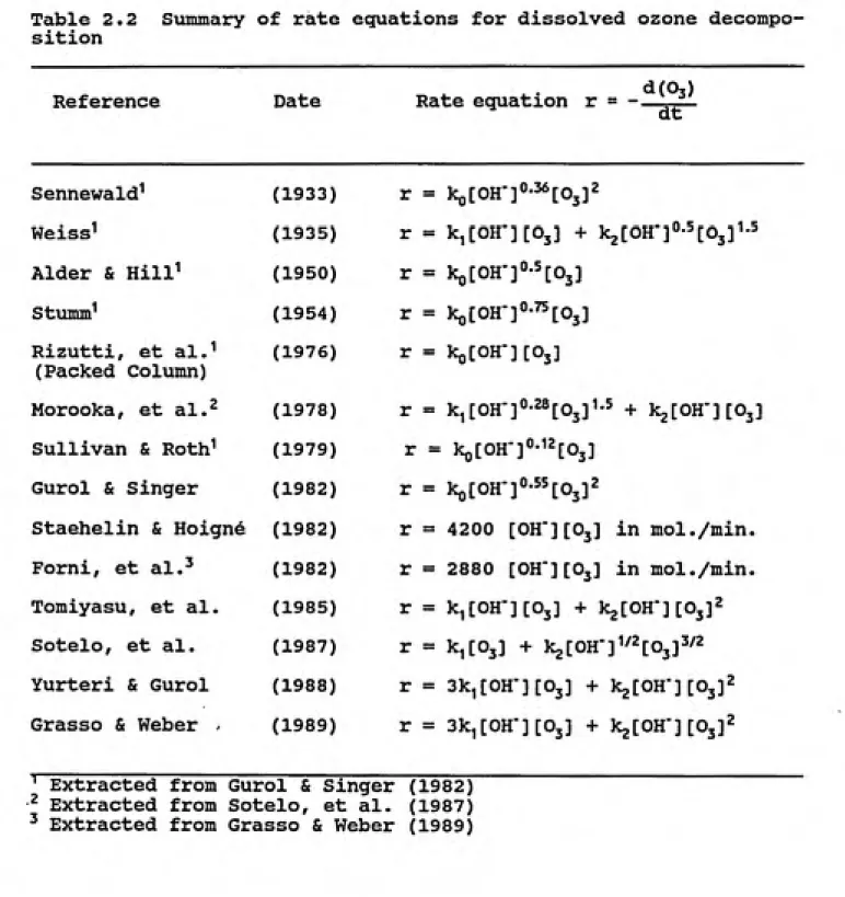
equations. Figure 4.2 depicts first-order ozone decomposition at
various pH values. Table 4.2 lists the corresponding first-order
rate constants and the theoretical 3k,[OH'] values for comparison
(based on Staehelin and Hoigne (1982)). Also listed are the rate
constants determined from a second-order fit of the data. It is
clear from the figure and regression coefficients (r^ values)
listed in the table that the first-order model fits the experi¬
mental data very well. Figure 4.2 shows that the rate of ozone
decomposition increased with increase in pH. This is due to the
increase in hydroxide ion concentration which initiates the ozone
decomposition cycle (see Figure 2.1 in Chapter 2). A number of
0
-2 —
o ^ -3
-4 —
-5
0 10 20 30 40
Time (minutes)
50 60
Figure 4.2 Effect of pH on ozone decomposition in water
reported the same observation. The extent of increase in the
first-order rate constant is proportional to the hydroxide ion
concentration ([OH']) in the test solutions. Figure 4.3 illus¬
trates this observation. Staehelin and Hoigne (1982) and other
researchers (see Table 2.2 in Chapter 2) have reported similar
results. It is important to note that the first-order rate
constant did not vary linearly with hydroxide ion concentration as
expected based on the k/ = 3k,[OH'] relationship. This behavior
could be due to other initiation reactions occuring due to the
presence of impurities in the test solution.
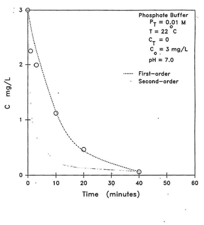
Figure 4.4 illustrates the second-order plots and Figure
4.5 depicts the predictions of the first-order and second-order
models. These figures clearly show the lack of fit of the second-order model.
In order to verify the first-order nature of aqueous ozone decomposition, the effect of initial ozone concentration was studied. Experiments were conducted at pH 7 with initial ozone
concentrations varying from 0.3 mg/L to 3 mg/L. The experimental
results illustrated in Figure 4.6 indicate that the first-order
ozone decomposition rate constant, represented by the slope of the line, is independent of initial ozone concentration. However, the slight deviation from first-order behavior at low residual ozone concentrations suggests a weak effect of the second-order rate con¬
stant from the mixed-order model which has been lumped into the
c E
U.'^UU
-Phosphate Buffer
Pj = 0.01 M
T = 22 °C
0.300 -
-C^ = 0
C^ = 3 mg/L
•
0.200 -
-•
0.100
-•
•
•
0.000 - 1 1 1
7 pH
8
Figure 4.3 Effect of pH on first order rate constant of ozone
50
40
-E
o
o
30
--I 20 u
D
10 —
oiiiS^
0 10
D
i
Phosphate Buffer
A
^
20 30 40Time (minutes)
T =
= 0.01 M
0
22 C
c
0
= 0
= 3 mg/L
pH
o 5.5 • 6.5
A 7.0 A 8.0
n 8.5
50
()
60