1150.pdf

CONTENTS

INTRODUCTION...1

Local Exhaust Ventilation...2

Capture Velocity...9

Empirical Equations for Calculating Capture Velocity..11

Problems with the Capture Velocity Design Approach....16

3-Dimensional Modelling of Hood Flows...18

Presence of a Body in Front of the Exhaust Inlet...20

Capture Efficiency...24

THEORY...27

OBJECTIVE AND PURPOSE...29

EXPERIMENTAL METHOD...31

General Description...31

Hood, Ductwork, and Fan Arrangement...33

Air Flow Through the LEV System...33

Sulfur Hexafluoride Gas Metering System...35

Use of Mannequin to Model Worker...36

Use of MIRANs to Measure SFj Concentration...37

Capture Efficiency Measurement and Duct Sampling Location...39

Experimental Procedure...39

RESULTS...43

Overall Results...4 3 Difference Between Experimental Runs #1 and #2...43

Decision to Use Run #2 Data to Analyze the BZC -Capture Efficiency Relationship...50

Buildup with Room SF, with Time...51

Relationship Between BZC and Capture Efficiency...52

Capture Efficiency and Capture Velocity...54

DISCUSSION OF RESULTS...65

Application of Results to Real Work Situations...65

Effect of SFj Leakage...68

Relationship Between BZC and Capture Efficiency...70

Relationship Between BZC and Calculated Capture

Velocity...72

Time Dependency of the Relationship Between BZC

and Capture Efficiency...74

Effect of Various LEV Parameters on the BZC - Capture

Efficiency Relationship...76

Test of Difference in Mannequin BZC Based on Position.84

Relationship Between BZC and Capture Efficiency...91

Capture Efficiency Versus Capture Velocity...91

Time Dependency of BZC and Capture Efficiency...92

Effect of Variation in LEV Parameters on the BZC

-Capture Efficiency Relationship...93

Increase the Mannequin's BZC of SF,...96

Show Reproduceability in the Results of this

Experiment...97

Measurements of Capture Velocity...98

Simultaneous Measurement of BZC and Capture

Efficiency...99

#*

Industrial hygienists attempt to protect workers from

occupational health stresses using three well-known methods:

recognition, evaluation, and control. If an occupational health

hazard has already been identified (eg. air sampling for a given

chemical) and quantified, the industrial hygienist's attention

necessarily shifts to controlling the worker's exposure to that

hazard. Methods of controlling worker exposure to physical or

chemical health hazards include engineering and administrative

controls, and personal protective equipment.

Engineering controls remove the responsibility for

protection against health hazards from the worker by physically

changing the process which generates the hazard. Examples of

such types of control include isolation of the process,

substitution of hazardous process chemicals, automation (eg.

robotics), ventilation, or elimination of the process entirely.

Engineering controls are mandated by law and must be used when

feasible.

Administrative controls, on the other hand, attempt to limit

the worker's exposure to a given health hazard by decreasing the

time of exposure (eg. rotating shifts) or changing work

practices. Education, training and supervision can also be

thought of as types of administrative controls.

Finally, personal protective equipment (ppe) is the least

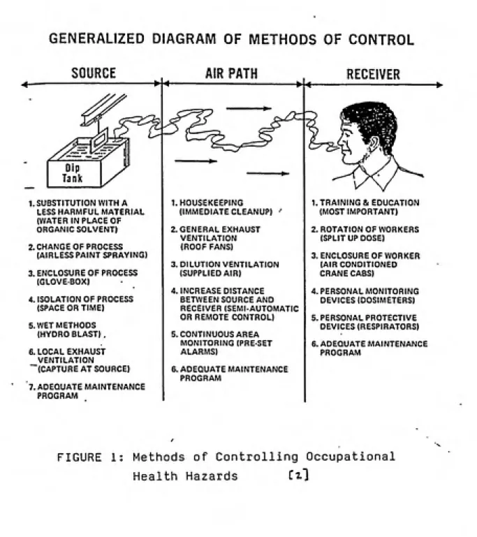
respirator or hearing protection). Figure 1 lists several

methods of control available to the industrial hygienist for

protecting workers against health hazards.

Perhaps the most widely used engineering control in

protecting workers from airborne chemical hazards (i.e. gases,

vapors, or aerosols) is ventilation. Exhaust ventilation systems

are typically classified as being either general or local [1].

General industrial ventilation (or dilution ventilation) systems

are used to flush out a given work space with large amounts of

air for the control of low toxicity contaminants or heat. A

supply ventilation system is used in conjunction with general

exhaust ventilation to replace exhausted air from the plant.. According to the ACGIH [11, "the use of dilution ventilation for health has four limiting factors: (1) small quantity of

contaminant generated, (2) workers should be far away from the contaminating source, (3) low toxicity contaminant, and (4) the

evolution of contaminants must be reasonably uniform." LOCAL EXHAUST VENTILATION AS AN ENGINEERING CONTROL

Local exhaust ventilation (termed "LEV" for the remainder of the report) acts on the principle of placing the contaminant

source close enough to an exhaust system inlet so that the

contaminant is "captured" by the ventilation system and removed from the worker's breathing zone. LEV is the preferred method of contaminant control because it is more effective than dilution ventilation and results in lower exhaust flow rates and lower

heating costs. Ideally, only polluted air should be collected

GENERALIZED DIAGRAM OF METHODS OF CONTROL

SOURCE

.-1 AIR PATH RECEIVER

y^

ͣ

4---1

^

_{^&P jT}

' <^K

/^^^\

-^^-^-Ct---^^l^ .;.'K ll

-Dip

Tank

}

_{~X y^K,.^^}

X

_'\X\/^'^

1. SUBSTITUTION WITH A 1. HOUSEKEEPING 1 TRAINING & EDUCATION LESS HARMFUL MATERIAL (IMMEDIATE CLEANUP) ' (MOST IMPORTANT) (WATER IN PLACE OF

ORGANIC SOLVENT) 2. GENERAL EXHAUST 2 ROTATION OF WORKERS

VENTILATION (SPLIT UP DOSE) 2. CHANGE OF PROCESS (ROOF FANS)

(AIRLESS PAINT SPRAYING) 3 ENCLOSURE OF WORKER

3. DILUTION VENTILATION (AIR CONDITIONED 3. ENCLOSURE OF PROCESS (SUPPLIED AIR) CRANE CABS)

(GLOVEBOX)

4. INCREASE DISTANCE 4 PERSONAL MONITORING 4. ISOLATION OF PROCESS BETWEEN SOURCE AND DEVICES (DOSIMETERS)

(SPACE OR TIME) RECEIVER (SEMI-AUTOMATIC

OR REMOTE CONTROL) 5 PERSONAL PROTECTIVE

5. WET METHODS _{DEVICES (RESPIRATORS)}

(HYDRO BLAST) , 5. CONTINUOUS AREA

MONITORING (PRESET 6 ADEQUATE MAINTENANCE

6. LOCAL EXHAUST ALARMS) PROGRAM

VENTILATION

(CAPTURE AT SOURCE) 6. ADEQUATE MAINTENANCE

PROGRAM

7. ADEQUATE MAINTENANCE

PROGRAM

of the ventilation system [27].

The ACGIH Ventilation Manual lists four elements of a basic LEV system: the hood, the duct, the air cleaning device, and the

fan [1]. Figure 2 diagrams a typical LEV system with its

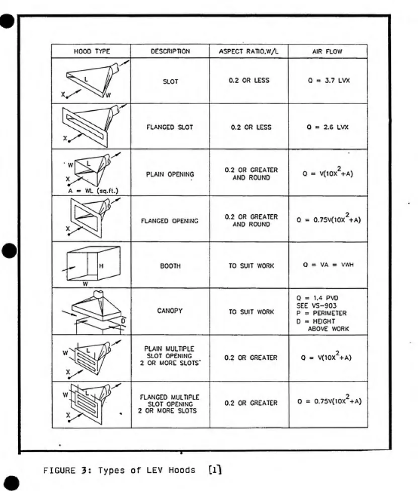
component parts. The hood is defined as the point of entry into the exhaust ventilation system and it includes all suction

openings, regardless of configuration. The purpose of the hood is to collect the contaminant in an air stream directed toward the hood. Examples of various types of LEV hoods can be found in

Figure 3 [1]. The purpose of the duct is to transport the

contaminant through the ventilation system to the air cleaning device. If the contaminant is a particulate, close attention

should be paid to providing a minimum design duct velocity to effectively transport the particulate without settling. The air

cleaning device removes the contaminant from the air stream. Examples of air cleaning devices include cyclones, fabric

filters, or air scrubbers. Finally, the fan produces the required air flow to overcome all pressure losses in the

ventilation system due to friction, hood entry, and fittings. There are two general categories of LEV hoods: enclosing hoods and exterior hoods. An enclosing hood completely or

partially encloses the operation which produces the contaminant. Figure 4 illustrates the use of completely or partially enclosing hoods [1]. Socha [421 lists five reasons why the use of

enclosing hoods in LEV is preferred: (1) lower exhaust volumes

DUCT HOOD

FAN

CLEANER

Figure 2 Elements of a Local Exhaust System, [i]

HOOD TYPE DESCRIPTION _{ASPECT RATIO,W/L} AIR FLOW

SLOT 0.2 OR LESS Q = 3.7 LVX

FLANGED SLOT 0.2 OR LESS Q = 2.6 LVX

A = WL (sq.ft.)

PLAIN OPENING 0.2 OR GREATER

AND ROUND 0 = V(10X +A)

FLANGED OPENING 0.2 OR GREATER

AND ROUND 0 = 0.75V(10X +A)

W

BOOTH TO SUIT WORK Q = VA = VWH

CANOPY TO SUIT WORK

Q = 1.4 PVD SEE VS-903 P = PERIMETER D = HEIGHT

ABOVE WORK

W PLAIN MULTIPLE

SLOT OPENING 2 OR MORE SLOTS'

0.2 OR GREATER _{0 = V(10X +A)}

FLANGED MULTIPLE SLOT OPENING 2 OR MORE SLOTS

0.2 OR GREATER Q = 0.75V(10X +A)

FIGURE 4: Completely or Partially Enclosing Hoods [i]

t

BELT

HOOD

ENCLOSING HOOD

O _{BELT ( O ) o'}

HOPPER

-/—^-HOPPER GOOD

ENCLOSE

-!ͣ—^

BAD

ENCLOSE THE OPERATION AS MUCH AS POSSIBLE. THE MORE COMPLETELY ENCLOSED THE SOURCE, THE LESS AIR REQUIRED FOR CONTROL.

(CX~^

SLOT

V

PROCESS

t

GOOD BAD

DIRECTION OF AIR FLOW

LOCATE THE HOOD SO THE CONTAMINANT IS REMOVED AWAY FROM THE BREATHING

ZONE OF THE OPERATOR.

can be used, and (v) a smaller air cleaning device can be used.

In other words, the use of an enclosing hood will add up to a lower capital cost to install the system and lower operating costs to achieve the same level of control as an exterior hood.

If it is not feasible to install an enclosing hood around the contaminant generating process, an exterior hood will be

necessary. Exterior hoods are located adjacent to the

contaminating process, without enclosing it. A sufficiently high

air flow must be provided through the exterior hood to produce an exhaust flow field out in front of the hood capable of

"capturing" the pollutant and overcoming its natural tendency to disperse [27].

The hood's orientation with respect to the location of the contaminant source and worker is also a very important

consideration in LEV. Ideally, the LEV hood should be located such that the flow field (suction) generated out in front of the hood directs the pollutant away from the worker's breathing zone. Figure 5 illustrates two types of hood configurations: one which pulls the contaminant away from the worker's breathing zone and the other which pulls the contaminant through the worker's

breathing zone [11. The type of contaminant present in a given

operation also influences the selection of hood orientation with respect to the contaminant source. If the contaminant is a gas, vapor, or fine particulate emitted with low source velocity, the

hood's location with respect to the contaminant source is not

critical. However, if the contaminant contains large

momentum), the hood should be placed in the path of source

emission. This type of exhaust inlet is sometimes referred to as a receiving hood.

When using exterior hoods to control worker exposure to

airborne pollutants, all sources of external air flow (other than the flow induced by the hood) should be minimized or eliminated

[1]. Examples of sources of external air flow include thermal air currents, motion of machinery, motion of material such as dumping, worker movement, and general room air currents.

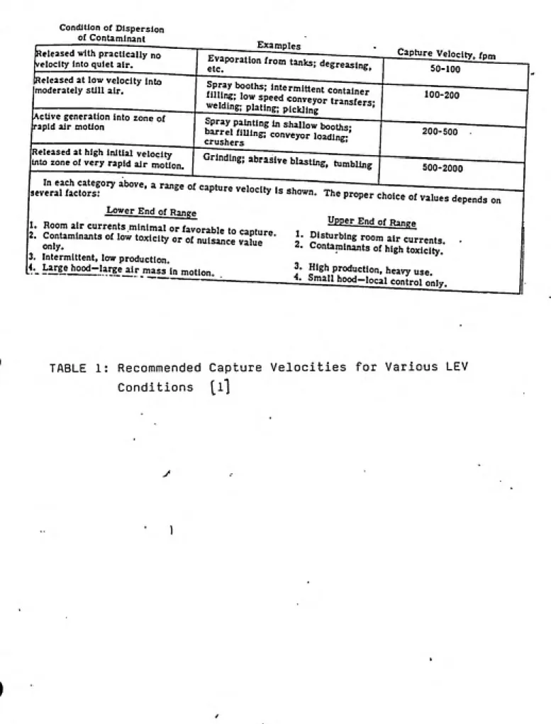
CAPTURE VELOCITY

The most widely used design parameter for LEV systems is the

concept of capture velocity. Capture velocity is defined as the air velocity required at a point to overcome the natural movement of the pollutant and draw it into the hood [451. Capture

velocity depends on the air flow rate generated by the LEV system and the configuration and location of the hood. Recommended

values of capture velocity have been tabulated for various LEV

conditions and is available in most books on LEV. Table 1

contains recommended values of capture velocity for various LEV conditions. Selection of the proper design capture velocity for a given operation depends on the conditions of contaminant

dispersion or release, the contaminant's toxicity, the presence

or absence of disturbing room air currents, the scale of the operation, and the size of the exhaust hood [1].

A slightly different approach to the capture velocity

concept was proposed by Hemeon [45] (1963) and is known as the

10

Condition of Dispersion

________of Contaminant

Released with practically no •elocity Into quiet air.

^ieleased at low velocity into

moderately still air.

Examples

Evaporation from tanks; degreasing,

etc.

Capture Velocity, fpm 50-100

AcUve generation into zone of

rapid air motion

Released at high initial velocity into zone of very rapid air motion.

---ͣ---___

Spray booths; intermittent container

filling; low speed conveyor transfers;

welding; plating; pickling

100-200

Spray painting in shallow booths;

barrel filling; conveyor loading;

crushers

Grinding; abrasive blasting, tumbling

200-500

500-2000

Lower End of Ranpe

1. Room air currents minimal or favorable to capture

onTy '°''*'''y °^ °^ ""'^^« vafue

Upper End of Range

only.

3. Intermittent, low production.

*\ Large_hood-large_air mas£in motion.

1. Disturbing room air currents.

2. Contaminants of high toxicity.

3. High production, heavy use.

4. Small hood—local control only.

TABLE 1: Recommended Capture Velocities for Various LEV

Conditions [l]

11

must not only exist at the source, but also at the null point. The null point is defined as the distance from the pollutant source to the point at which the pollutant release energy has

been expended and the velocity has decreased to that of random air currents in the room.

The current method of LEV system design for a given

industrial operation is to consult one of the VS-prints in the ACGIH Ventilation Manual [1]. Each VS-print applies to a ͣ

specific operation and represents a ventilation design which has proved successful in past operations. Once a LEV system design has been chosen, the required air flow to produce a given capture velocity is calculated using one of several empirical design

equations. Empirical equations for the centerline velocity gradient in front of various hood configurations have been

devised by Dalla Valle, Silverman, Fletcher, Garrison, and others

[33] .

EMPIRICAL EQUATIONS FOR CALCULATING CAPTURE VELOCITY

Using a specially modified Pitot tube in the 1930's, Dalla Valle [33] pioneered work on the aerodynamic characteristics of plain and flanged circular and rectangular hoods. Dalla Valle

focused his worJc on exhaust inlets with a width to length ratio

(WLR) of 0.2,or greater. Using the Pitot tube, Dalla Valle

mapped equal velocity contours for plain and flanged circular and

rectangular hoods. His exact equation for plain exhaust inlets

12

(V/V. i,.^, = l/{lQ^/h + 1) (1)

where V = centerline capture velocity (fpm), V, = average hood

face velocity = Q/A (fpm), X = source to hood distance along the

centerline (ft), and A = hood inlet area (ft'). To solve for the

required hood flow rate to produce a given centerline capture

velocity. Equation (1) can be re-written into the form found in

the ACGIH Ventilation Manual [1]:

Q = V(10X* + A) (2)

where Q = exhaust air flow rate (cfm). Dalla Valle assumed that flanges around exhaust Inlets reduced the required air flow by 25% over flanged inlets. In other words, centerline capture velocities were about 133% higher for flanged over plain inlets. This assumption resulted in his formulation for flanged hoods:

(V/V, i,„,., = 1.33/{10xyA + 1) (3)

where all of the variables are the same as described for Equation

(1). The ACGIH reports Dalla Valle's equation for flow through flanged hoods as:

Q = 0.75V(10X' + A) (4)

Unfortunately, Dalla Valle's equations do not describe the

variation of centerline capture velocity as a function of WLR

(W/L). Also, a basic assumption of Dalla Valle's equations is that the velocity at the center of the hood face is equal to V„ = Q/A. This does not account for the observed velocity increase at the center of the hood face due to the vena contracta formed at

the inlet.

In the 1940's, Silverman studied circular and narrow slot

13

centerline velocity gradient produced in front of narrow slot hoods complemented Dalla Valle's earlier work and also have found wide application in LEV design:

Plain Q = 3.7LVX (5) Flanged Q = 2.6LVX (6)

where Q = exhaust air flow rate (cfm), L = length of the slot (ft), V = centerline capture velocity (fpm), and X = centerline source to hood distance (ft). A problem with these equations for narrow slot openings is that they "blow up" as X approaches zero.

In other words, Silverman's equations are undefined for capture

velocities close to the hood face. In addition, Silverman's equations also do not describe centerline capture velocity as a function of WLR.

In recent times, other researchers have examined the

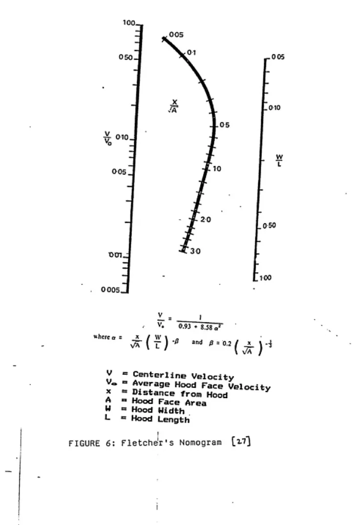
empirical relations developed by Dalla Valle and Silverman and have modified them. Fletcher [27] investigated plain rectangular hoods ranging from square to narrow slots (i.e. 0.063 < WLR < 1). He varied the WLR of these hoods for the specific purpose of

examining the change in centerline capture velocity with decreasing WLR. By doing so, Fletcher discovered that for a

given face area and volume flow, the capture velocity at a fixed

point in front of the hood decreases as the WLR decreases (i.e.

or as the aspect ratio (L/W) increases). Fletcher's equation for centerline capture velocity in front of plain rectangular hoods

takes a non-dimensional form:

VA/Q = V/V, = 1/(0.93 +8.58o?) (7)

14

V = centerline capture velocity (fpm), A = hood face area (ft'), V„ = average hood face velocity (fpm), Q = exhaust air flow rate

(cfm), W = width of rectangular hood (ft), and L = length of rectangular hood (ft). To facilitate calculations of capture

velocity using this equation, Fletcher created a nomogram giving

V/V, in terms of X/(A)''-»and W/L. Figure 6 contains Fletcher's

nomogram for computing centerline capture velocities of plain

rectangular hoods.

Later, Fletcher [37, 483 expanded his work to investigate

the effect of flanging and adjacent planes on LEV hoods. These investigations led to Fletcher's conclusions that both flanging and the placement of adjacent planes next to local exhaust hoods

increased the capture velocity at a point in front of the inlet

(with flow rate and hood configuration being held constant). He

also reported that the optimum hood flange width was equal to the square root of the hood face area.

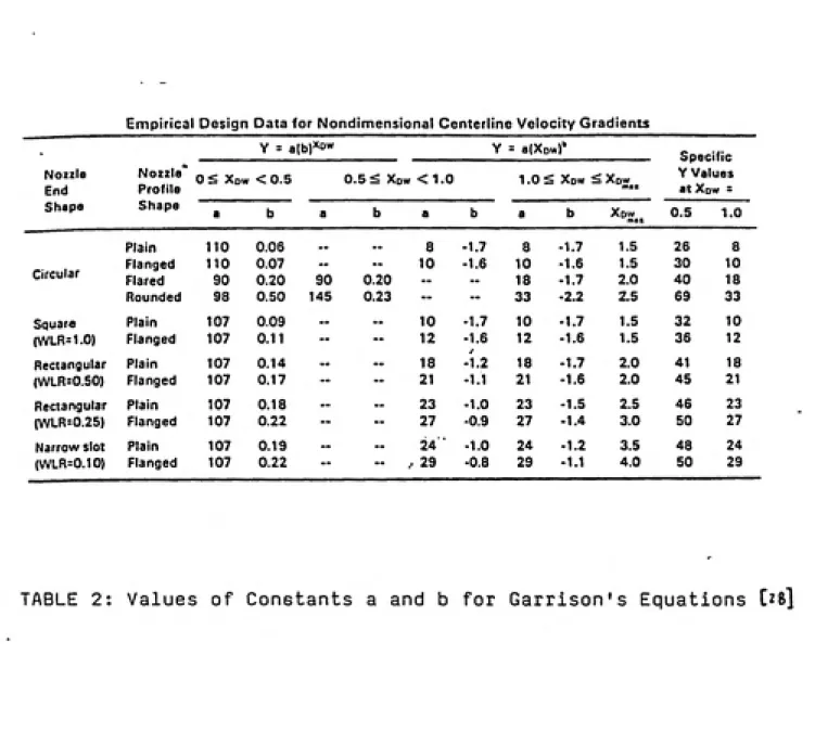
Within the last decade. Garrison [28, 33] studied plain and

flanged circular and rectangular hoods for high velocity, low

volume (HV/LV) exhaust ventilation. His analytical approach involved the use of two simple dimensionless equations to describe the centerline capture velocity gradient. The

application of each equation depends on the distance the

contaminant source is from the exhaust inlet:

(V/V, )„.. = a(b)"'' (8)

(V/V, ),„= a(Xdw)'' (9)

15

TOO.

0 50.

010.

0 05.

0O5

X>01.

.005

.010

W L

.0 50

0 005.

.100

where a

Vo 0.93 + 8.58 a'

^ ( - j -/J and ^ -- 0-2 ^ ^ \

V

X

A U L

= Centerline Velocity

» Average Hood Face Velocity

= Distance from Hood

= Hood Face Area

s Hood Width

- Hood Length

16

rectangular hoods). In Equations (8) and (9), a and b are

empirically determined constants based on nozzle end shape,

nozzle profile shape, and range of Xdw. Table 2 contains values

PROBLEMS WITH THE CAPTURE VELOCITY DESIGN APPROACH

Empirical equations which predict centerllne capture

velocity for various exhaust inlet configurations are simple to

cipply, but do not take Into account many "realities" of LEV.

(i) Inability to predict contaminant concentration: The

use of capture velocity offers no way to estimate the

concentration of contaminant at arbitrary points in the vicinity

of the source.

(11) Off-design performance of conventional design: LEV

systems are seldom constructed or operated exactly as specified

in the design. Practical considerations and administrative

decisions often arise which require a change in the system

dimensions or exhaust flow.

(ill) Generalization of acceptable designs: Even if a

LEV design is effective in controlling a contaminant to OSHA

standards, there is no way to scale the design geometrically to

protect against different concentrations of the contaminant (eg.

if the PEL is lowered).

(Iv) New configurations: In the case of new Industrial

operations, where no proven designs or published material Is

17

Empirical Design Data for Nondimensional Centerline Velocity Gradients

Y = a(b)XDW Y = a(XD«f

Specific

Nozzle End

Nozzle Profile

Shape

0< Xdw <0.5 0.5 < Xdw<1.0 1.0< Xdw <Xdw Y Values at Xdw = Shape a b a b a b a b Xdw 0.5 1.0

Plain 110 0.06 .. _. ₈ -1.7 8 -1.7 1.5 26 8

Flanged 110 0.07 - — 10 -1.6 10 -1.6 1.5 30 10 Circular _Flared 90 0.20 90 0.20 — - 18 -1.7 2.0 40 18 Rounded 98 0.50 145 0.23 -- " 33 -2.2 2.5 69 33 Squar« Plain 107 0.09

— — ₁₀ -1.7 10 -1.7 1.5 32 10

|WLR=1.0) Flanged 107 0.11 -- -- 12 -1.6 12 -1.6 1.5 36 12

Rectangular Plain 107 0.14 — — ₁₈ •1.2 18 -1.7 2.0 41 18

(WLR=0.50) Flanged 107 0.17 -- -- 21 -1.1 21 -1.6 2.0 45 21

Rectangular Plain 107 0.18

— — 23 -1.0 23 -1.5 2.5 46 23

(WLR=0.25) Flanged 107 0.22 -- -- 27 -0.9 27 -1.4 3.0 50 27 Narrow slot Plain 107 0.19 — — 24 -1.0 24 -1.2 3.5 48 24

(WLR=0.10) Flanged 107 0.22 -- " 29 -0.8 29 -1.1 4.0 50 29

18

(v) Physical inconsistency: The concept of capture

velocity is not consistent with the laws of fluid mechanics. Contaminants move because the medium in which they are immersed

is moving. In the case of particle, there is additional movement because of gravity, inertia, and electrostatic forces. In the case of gases and vapors, there is additional movement because of diffusion.

(vi) Economics: Capture velocity does not address the

economics of LEV system design by determining the optimum air

flow which will provide control of the contaminant (at minimum

cost).

Other LEV researchers point out that capture velocity does

not address the issue of pollutants released at points other than the hood centerline. Ellenbecker et al [43] explain that capture

velocity does not account for the presence of cross drafts or other air disturbances. Garrison [31] points out that capture velocity says nothing about how the presence of obstacles (i.e. a worker's body) in front of an exhaust inlet affects the capture of contaminant. Most important, capture velocity does not allow for predictions of the principal index of LEV performance, the breathing zone concentration (BZC) of the worker.

3-D MODELING OF HOOD FLOWS - POTENTIAL FLOW THEORY

Recently, attempts have been made to characterize the three

dimensional nature of local exhaust hood flows. The ability to

predict the velocity vector at any point (i.e. not only the

19

and others [363. Such models would allow, through vector

addition, prediction of exhaust flow streamlines in the presence of a uniform cross draft. However, the difficulty in modeling 3-dimensional air flows into exhaust hoods is that equations must satisfy the conservation of mass (continuity equation), the

conservation of energy, the conservation of linear momentum (Navier-Stokes) and thermodynamic equations of state. Unless simplifying assumptions and boundary values are specified, these

partial differential equations cannot be solved analytically. Many researchers have made the assumption that the flow into unobstructed exhaust inlets follows potential flow theory.

Potential flow is valid if the fluid is incompressible,

irrotational, and inviscid. Incompressible flow signifies that there is no accumulation of flow through a volume. In other

words, the fluid density does not change. For irrotational flow, the fluid is said to have no angular velocity or vorticity (i.e. spinning motion). Finally, if the fluid is inviscid, there are no viscous (frictional) forces acting. Clearly, the flow into the hood must be unobstructed for potential flow theory to apply because flow around a worker's body will cause frictional forces to act on the fluid and fluid vorticity will be observed. A detailed description of the derivations of equations used to describe potential flow theory is beyond the scope of this

report. However, the reader is referred to the fluid mechanics

text by White [3] for a detailed treatment.

20

Ellenbecker [32, 36] have proposed analytical solutions for the velocity vector at any point in front of a flanged circular hood.

In 1970, Tyaglo and Shepelev [36] formulated a solution for the

velocity vector at any point in front of a flanged rectangular

hood. In 1987, Jansson [36] did the same for a flanged slot opening.

PRESENCE OF A BODY IN FRONT OF THE EXHAUST INLET

While these solutions contribute a great deal to the

understanding of LEV as a 3-dimensional phenomena, the problem of

a worker standing directly in front of an exhaust inlet is not

addressed in these models. Potential flow theory does not hold

for a body placed in the flow field of an LEV hood because the boundary conditions of LaPlace's Equation are violated [31.

When a fluid flows past a bluff body, a boundary layer forms around the body. The boundary layer is defined as the distance

from the body's surface (where air velocity at the surface equals zero - the no-slip condition) to a point away from the body where 99% of the free-stream velocity has been achieved. At low

Reynolds numbers (Re) the boundary layer thickness is large, but

for turbulent flow past the body (i.e. high Re), the boundary

layer is thin. Within the boundary layer, viscous forces are

acting on the fluid. However, outside of the boundary layer, the

fluid flow may be assumed to be inviscid.

As a fluid attempts to flow around a body, such as a cylinder, the boundary layer encounters an adverse pressure

gradient (i.e. increasing pressure in the direction of flow).

21

boundary layer separates from the cylinder into a low pressure vortical mixing zone near the downstream side of the cylinder.

Figure 7 illustrates the phenomenon of boundary layer separation

from a cylinder in a uniform flow field. Because this reverse

flow (mixing) region is a zone of low pressure, surrounding air from outside the region becomes entrained into it. If the body is axisymmetric (i.e. more 3-dimensional, like a sphere), the

reverse flow region forms a recirculation bubble downstream of

the body. If the body is 2-dimensional, like a long cylinder or

a person's body, alternate vortices shed downstream of the body forming a Karman vortex street [11]. In the field of fluid

mechanics, several studies have been performed involving various bluff body shapes placed in a uniform (i.e. constant velocity) flow field [8, 9, 11, 19, 20, 21, 23]. Many of these studies involve determining the flow of air pollutants around buildings and clusters of buildings [12, 13, 14].

Experiments have been performed to determine the transport mechanisms of pollutants into and out of this zone of

recirculation [8, 9, 11, 12, 19]. For axisymmetric

(3-dimensional) bluff bodies placed in a uniform flow field, the primary mechanism of pollutant transport into and out of the

recirculation bubble is turbulent diffusion. On the other hand,

«

for 2-dimensional bluff bodies placed in uniform flow, the

principal mechanism of pollutant transport is the periodic

shedding of vortices [11].

If a worker's body is placed in a uniform flow field, such

m

22

Thin front -.

boundary layer

Outer stream grossly

perturbed by broad How

separation and wake

23

separation and vortex shedding would be expected to occur. If

the contaminant source is located between the worker's body and

the exhaust flow inlet (i.e. usual orientation for most LEV applications), and the source coincides with the reverse flow

zone formed by boundary layer separation, the contaminant may be

recirculated back into the worker's breathing zone. George [49] performed experiments in this regard using a mannequin holding a

tracer gas source inside a wind tunnel. His experiments demonstrated that measured BZC was less when the mannequin's

shoulders were parallel to the direction of flow (i.e.

mannequin's side to flow). In this situation, the reverse flow

region forms downstream near the mannequin's side where there is no oppurtunity to interact with the contaminant. Similar results

have been demonstrated in a shielded metal arc welding study

performed by Tum Suden [50].

Very little research has been performed, however, for the case of a worker placed in the accelerating flow field of a LEV hood. In this case (as in most LEV situations in industry) the flow around the body is not uniform, but accelerating into the hood. The flow field for a LEV hood falls off very quickly as the distance from the hood face is increased. Furthermore, the

velocity field in front of a local exhaust inlet would be

converging on the hood from all directions, rather than from one

reverse flow would still be expected to occur, but perhaps not to

24

CAPTURE EFFICIENCY

Since capture velocity is not an adequate measure of how well a LEV hood actually performs, Ellenbecker et al [43]

introduced the concept of capture efficiency to describe hood performance. Capture efficiency is defined as the fraction of airborne contaminants generated by a source that is captured by

the LEV system controlling it. This concept is represented as: n, = G'/G (10)

where n, = hood capture efficiency, G' = LEV contaminant capture

rate (g/sec), and G = contaminant generation rate (g/sec). In a similar manner, Flynn et al [44] describe the rate of escape of contaminant into the workplace as:

G'' = (1 - n,)G (11)

where G*' = the effective contaminant generation rate into the room atmosphere (g/sec). Since capture efficiency is related directly to the concentration of airborne contaminant present in the room, and capture velocity is not, capture efficiency

represents a significant advance in the design of LEV systems [43]. Even more important, if capture efficiency can be shown to be functionally related to worker BZC (i.e. the main parameter of interest), then capture efficiency may be a very useful LEV

design parameter. On the other hand, if the contaminant is

pulled through the worker's breathing zone prior to being

captured by the hood, then capture efficiency may not be an

important design parameter for LEV.

•

•

25

centerline source to hood distance (Z,), cross draft velocity

(V,), and source temperature (T): '

n, = f (Q, A, Z ., Vrf T) (12)

If source temperature can be Ignored, dimensional analysis

indicates that capture efficiency depends on the functional group

9-g = (V,/\J)*(^A-"-» )" (13)

In Equation (13), V, = average hood face velocity, and a and b

are empirically determined constants. Several limiting

conditions must be satisfied for n, to depend on functional

n, = 0 as 5 approaches infinity

n, = 0 when Y = 0

n, = 0 when V approaches infinity

n, = 1 when J = 0 n, = 1 when y = 0

Ideally, the last condition can only be satisfied for an enclosure where there are absolutely no cross drafts or air

currents. In reality, room air currents will always be present.

If we were to evaluate capture efficiency with respect to

previously mentioned capture velocity "deficiencies", n, would

fare better than V^ on most deficiencies, but not all. Since

capture efficiency describes the ratio of contaminant capture to

contaminant generation, and says nothing about how a hood

26

holding the contaminant source, and then again when the source was placed inside the hood, a LEV system could be designed to operate at its lowest possible flow rate to achieve a given

capture efficiency. In this respect, capture efficiency could be used to design the "most economical" ventilation system. Since capture efficiency is not based on empirical centerline design equations, but is a measured parameter, it can be used to design systems in which there is a cross draft, pollutants are released off of the centerline, and when a worker (i.e. bluff body) is

standing in front of the hood. However, n, still falls short on

"predicting contaminant concentrations", and geometrically

scaling ventilation systems to protect against new concentrations of a contaminant (eg. lower OSHA PEL).

Several authors have created models which calculate capture efficiency by using (BASIC) computer programs to predict the streamlines entering various hood configurations in the presence of a uniform cross draft [41, 44, 46, 47]. At the present time,

however, no attempts have been made to simultaneously measure capture efficiency and worker BZC with the aim of examining the relationship between these two parameters. This work will do

27

As mentioned earlier, capture efficiency is the ratio of the exhaust hood capture rate of contaminant to the contaminant

source generation rate. Since capture efficiency provides a

measure of the amount of contaminant which escapes into the room, it may be inversely related to the BZC of the worker. That is, as capture efficiency increases, worker BZC should decrease (and

vice versa).

The theoretical inverse relationship between BZC and capture efficiency can be demonstrated by relating BZC to the volume of a gaseous contaminant present in the room after a source generation

time, T. If a source is generating contaminant (at a constant flow rate) in a one inlet, one outlet (hood) room under the influence of a LEV system, and no other sources of dilution ventilation coming into the room, the volume of contaminant present in the room after a time, T, is described by the

relation:

f'

V. = Q, \ (1 - n, ) dt (14)

where V, = volume of contaminant present in the room (liters),

Q, = volumetric flow rate of contaminant source (liters/min),

n, = hood capture efficiency, T = total time of contaminant

generation, and dt = incremental time over which the integral is

evaluated. Note, Equation (14) does not apply to most "real

life" industrial situations because there is always going to be

some amount of dilution ventilation present. This equation,

•

28

Similarly, the concentration of contaminant present In the room

after a time, T, can be represented as: i./Y„. \

C(T) = Q./Y„. \ (1 - n,)dt (15)

ͣ

'o

where C(T) is the room concentration of contaminant after a time, T, and V,,„ is the room volume (liters).

In theory, the worker's instantaneous (final) BZC, measured

at time t = T should be proportional to the volume of contaminant

present in the room at time T:

BZC„,„ c< V..,„.,^.. , (16)

If a time weighted average value of capture efficiency over time T can be measured. Equation (14) can be approximated as:

(1 - n ,)dt = TQ,(1 - n ,) (17)

where n, = 1/T \ r^ dt (18)

0

T = total time of source generation (mln.) and n, = time weighted

efficiency over a contaminant generation time, T, and also

-"liT

29

OBJECTIVE AND PURPOSE

The primary objective for conducting this research is to

establish whether a relationship exists between worker breathing

zone concentration (BZC) and local exhaust hood capture

efficiency. This research seeks to determine the nature of this relationship as well as how various LEV system parameters, such

as position in front of a flanged circular hood (FCH), hood flow

rate, hood diameter, and source to hood distance, affect the

association between BZC and capture efficiency. In particular, this study will investigate whether worker BZC and capture

efficiency are inversely related. In other words, are high values of worker BZC associated with low values of hood capture

efficiency (and vice versa)? The overall purpose is to determine

whether capture efficiency, as a LEV design parameter, is a

better predictor of worker BZC than the widely used design

parameter of capture velocity. The correlation between measured values of BZC and capture efficiency will be compared to the

correlation between BZC and calculated values of Dalla Valle's

capture velocity.

Another important goal of this study is to examine how the

placement of a worker's body (i.e. back to flow - 180 degrees, or side to flow - 90 degrees) in front of a local exhaust hood

affects the worker's breathing zone concentration of contaminant.

Specifically, this research will investigate the effect of boundary layer separation and reverse flow on a contaminant placed downstream of an anthropometric mannequin (simulating a

30

hood. The hypothesis to be tested in this experiment is that the worker's BZC in the 180 degree position will be higher than the

BZC when the mannequin is in the 90 degree position due to the interaction of the reverse flow region and the contaminant

source.

To accomplish the objectives of this research, the following

experiments will be performed:

(i) Conduct laboratory experiments which measure

mannequin BZC (position 180 degrees) and hood capture efficiency for various combinations of FCH diameter, hood flow rate, and

source to hood distance.

(ii) Repeat all above laboratory experiments for the case where the mannequin's position is 90 degrees (i.e. side to

flow).

^1

31

EXPERIMENTAL METHQP

GENERAL DESCRIPTION

To accomplish the research objectives, an experiment was

devised which allowed the measurement of worker BZC and hood

capture efficiency over a given period of time. The diagram of the experimental setup used in this work can be found in Figure 8. An anthropometric mannequin was used to simulate a worker holding a contaminant source in front of a flanged circular local exhaust ventilation hood. Neutrally buoyant sulfur hexafluoride

(SF,) tracer gas was used to represent any gaseous contaminant

source. The mannequin was positioned in front of the hood such

that the contaminant source was on the hood centerline. The

contaminant source to hood distance was measured as Zj. The flow

rate through the ventilation system was adjusted with a blast gate and measured with a manometer placed across a calibrated

orifice meter. SF^ gas was metered through a calibrated

rotameter through copper tubing to a wand and diffuser stone

which was placed in the hands of the mannequin. The BZC and duct

concentration (i.e. for capture efficiency) of SF, were measured

with two mobile infrared absorption analyzers (MIRAN's) connected to a Metrosonics Datalogger. Capture efficiency was measured as the ratio of duct concentration when the source was in the

mannequin's hands to the duct concentration when the source was placed in the hood.

Hood flow rate, flanged circular hood (FCH) diameter, contaminant source to hood distance, and mannequin position in

it\fter ^N«Me : ^ETKp

FIGURE 8

EXPERIIIENTflL 5ETUP

SF6 Cylinder

Glass Sampling Til be

K o t(a m e t e r

Orifice

12 in FflH r

1

bin

Ce^-kr|;r^Fla n g e d

tlicro manometer

K)

Q r/J]

HIRRH Ifl CBZC) HIRfiH I (ETfl>

33

Hood Flow Rate, Q^ = 100, 300, 535 cfm FCH Diameter, D^ = 4, 9, 12 inches

Contaminant source - Hood Distance, Zj = 0.5, 0.75, 1.25 ft

Mannequin Position = 180 degrees (back to flow) =90 degrees (side to flow)

The flow rate of SFj as well as the source position in the

mannequin's hands were held constant. Two separate experimental runs were performed.

HOOD, DUCTWORK, AND FAN ARRANGEMENT

The hood dimensions, length of duct run, and size of ducts are given in Figure 9. A Size 129 SWSI Acoustafoil

(non-overloading) centrifugal fan was used to move the air through the ventilation system. Clean, circular, galvanized metal duct was used in the experimental setup. Ductwork on the downstreaift side of the fan was carefully sealed in heavy plastic and silicone caulking to minimize leakage of "captured" SF, gas into the room.

To prevent SF, exhaust gas from re-entering the building, the

exhaust outlet of the ventilation system extended 2.8 feet outside of the building and the wall opening was carefully

sealed. Despite these extensive measures aimed at preventing SF, leakage from the positive pressure side of the fan, some leakage was measured.

AIR FLOW THROUGH THE LEV SYSTEM

The air flow rate through the ventilation system was adjusted by the use of a blast gate (see Figure 9). LEV hood

^^ flow rates of 100, 300, and 535 cfm were chosen to provide a good

-""Hflier FlLef^)/lͣ^7e fit^t4

FIGURE 9

FCH

0

-1.1^

8'

Blcuft

^

i nT I____1

Orifice

-11.9'—»|2.8'-)|f

2.8'

5.2'

URLL

-.. I

So.niplifl'j Prote

Fan Outlet Co nV er g.

.= 1.3'

1 Fan Inlet

Diverging

Se c ti o n = 1.7'

35

capture efficiency relationship.

A manometer placed across a 4" ID, 6" OD sharp edged orifice meter was used to measure the flow rate through the ventilation system. The pressure drop across the orifice meter ("wg) was calibrated against flow rates computed from Pitot tube traverses. See Appendix 1 for details on the calibration of the orifice

meter.

SULFUR HEXAFLUORIDE GAS METERING SYSTEM

A neutrally buoyant, 10% mixture of SF, tracer gas was used to represent the contaminant gas for this experiment. This

concentration of SF, gas was chosen to provide a measureable

mannequin breathing zone concentration of SF, while, at the same

time, giving a good mid-scale absorbance reading for the MIRAN

measuring duct concentration of SF. (i.e. capture efficiency).

A neutrally buoyant gas mixture was chosen so the contaminant gas would not be heavier than air and sink out of the mannequin's breathing zone.

SF, gas was metered from a compressed gas cylinder by means of a regulator and two fine adjustment valves. A rotameter, placed in line between the cylinder and the wand and diffuser, was used to monitor the flow rate of SF,. The rotameter

calibration curve and detailed calibration procedure can be found

in Appendix 2.

To prevent leakage of SF, from the cylinder and associated connections, the cylinder was mounted on a dolly cart and placed

outside of the building during each experimental run. Copper

36

leakage of SF, gas. During an experimental run, all swagelock

connections, with the exception of the connection to the

diffuser, remained outside of the building (i.e. limited

The contaminant source consisted of a wand and diffuser

stone mounted in the hands of the mannequin. The diffuser stone

was a one-quarter inch diameter porous ceramic sphere. During

source generation, neutrally buoyant 10% SF, diffused through the

pores in the sphere in all directions (i.e. simulating 360 degree

source generation). A SF, flow rate of 0.782 1pm (0.027 cfra),

corresponding to a surface radial velocity of 19.8 fpm, was

chosen for this experiment. This flow rate of SF, was selected

to provide a raeasureable BZC of SF,, while at the same time

producing a velocity which should not interfere with contaminant

capture or produce a large amount of directionality to the flow

of the source (Note: an attempt was made to provide the lowest

SF, source flow rate which would still generate a raeasureable

USE OF MANNEQUIN TO MODEL WORKER

An anthropometric mannequin was used to model a worker

holding a contaminant source in front of a LEV hood. The

37

of the FCH. The location of the wand and diffuser in the

mannequin's hands represented a typical working position for a

worker holding some contaminant generating source (eg. a welder

with a welding torch). The position of the contaminant (SF,)

source in the mannequin's hands remained constant through all

experimental runs. The permanent source position in the

mannequin's hands can be described by the following measurements:

Source to Mannequin's Mouth Distance = 7 inches Source to Mannequin's Chest Distance = 4.5 inches

The mannequin was placed on a platform (approximately 8

inches tall) so that the position of the SF, source coincided

with the hood centerline. The surface of the platform contained

a grid, marked off in inches, such that the mannequin could be

easily positioned to achieve source to hood distances of 0.5,

0.75, and 1.25 feet. \

USE OF MIRANS TO MEASURE SF, CONCENTRATION

Two Wilks Mobile Infrared Analyzers (MIRANs) were used to measure the concentration of SF, in this experiment. A general description of the MIRAN's operation and settings used in this experiment can be found in Appendix 3. One MIRAN was used to monitor the BZC of the mannequin and the other was used to

measure the capture efficiency of the FCH.

Both MIRAN's were connected to a Metrosonics dl-714

Datalogger. In this setup, the voltage signal output from both

38

retrieved to an IBM XT or AT personal computer. Mannequin BZC and FCH capture efficiency were logged over a twenty minute

period. For specific information concerning the operation of the

Datalogger and the programmable settings used in this experiment, please see Appendix 4. The MIRAN calibration procedure and

calibration curves for both MIRANs can be found in Appendix 5.

The use of neutrally buoyant 10% SF, produced low mannequin

calibration points (i.e. MIRAN absorbances) for low

concentrations of SF, needed to be determined. To obtain calibration concentrations in the range of 0.01 - 0.02 ppm, a cylinder of 899 ppm SF, was used as the calibration gas. The Foxboro Corp. (i.e. manufacturers of the Wilks MIRAN) reports the

MIRAN lower detection limit of SF. to be 0.01 ppm. Since there

was some question concerning the stability of the MIRAN

absorbance (voltage) readings for such low concentrations of SF, , voltage versus time curves were plotted over a period of 1

minute. These plots can also be found in Appendix 5.

Two different air sampling flow rates were used to measure BZC and capture efficiency. An air sampling flow rate of 0.9

liters/min. was used to sample the mannequin's breathing zone

concentration of SF, . This flow rate was provided by a Rotron

SE2A-1 Spiral Exhauster Pump attached to the MIRAN. The BZC sampling flow rate was chosen because it is small enough not to

substantially influence the direction of contaminant generation

"^^ or interfere with reverse flow zone formation of contaminant.

39

no such constraints. A duct concentration sampling flow rate of

35.8 liters/min. was chosen to give a high chamber turnover rate

for the MIRAN (i.e. 1 air change/9.4 sec). In this way, the

duct concentration of SF, could be measured accurately without

having to wait long periods of time for the SF, concentration in

the MIRAN chamber to rise to the duct concentration.

CAPTURE EFFICIENCY MEASUREMENT AND DUCT SAMPLING LOCATION

In this experiment, hood capture efficiency was computed by

taking the ratio of duct concentration (of SF,) when the source

was in the mannequin's hands to the duct concentration when the

source was placed inside the hood. For each experimental run,

duct concentration of SF, was logged for 20 minutes with the

source in the mannequin's hands, and then logged for another 10

minutes with the source inside the hood (i.e. 100% capture).

Repeated tests showed that duct concentration measurements of SF,

were extremely stable.

The sampling location for capture efficiency was chosen to

be a point in the duct, downstream of the hood, where the SF,

concentration profile across the diameter of the duct was

determined to be linear. This duct sampling point was

experimentally determined by making a series of four ten-point

sampling traverses. Appendix 6 contains results of these

traverses as well as further information concerning the choice of

duct sampling location.

EXPERIMENTAL PROCEDURE

40

parameters:

Hood Flow Rate, Q^ = 100, 300, 535 c£m

FCH Diameter, D^ ^ 4, 9, 12 inches

Contaminant source to Hood Distance, Z, = 0.5, 0.75, 1.25 ft

Mannequin Position = 180 degrees (back to flow)

= 90 degrees (side to flow)

Figure 10 demonstrates how mannequin position in front of the FCH

was varied in this experiment. For each set of experimental

conditions, the mannequin was placed either 90 degrees to the

flow, termed as position 1, or 180 degrees to flow, termed as

position 2. Contaminant source flow rate and source position in

the mannequin's hands were held constant throughout the

experiment. BZC and capture efficiency measurements were logged

over a twenty minute sampling period. 108 total combinations of

the above experimental conditions were measured. Two repetitions

of each experimental combination (above) were accomplished.

Since the final mannequin BZC is theoretically correlated

with the volume of contaminant present in the room after 20

minutes, an average of the last four minutes of BZC data was used

to approximate "final BZC". Flynn developed a BASIC computer

program to extract and average the last four minutes of mannequin

BZC. A copy of this BASIC program can be found in Appendix f.

Prior to each experimental run, potential wind drafts in the

room were checked with a Taylor Model 3132 Rotating Vane

Anemometer. After each experimental run, the room concentration

of SF, was purged by opening the door and operating the wind

41

FIGURE 10

MANNEQUIN

P0S = 1

T

D

i

SOURCE

J

e

'h

42

tunnel flow rate corresponds to 29.02 air changes per hour (or

approximately 1 air change every two minutes). The room was

allowed to purge for approximately 20 minutes between each

experiment. Before the start of the next experiment, the MIRAN

(now monitoring room concentration of SF,) reading was checked

to ensure there was no measureable room cone, of SF,.

The two repetitions of the experiment, however, were not

exactly the same. In the first set of experiments, BZC and

capture efficiency were not logged until after the source flow

was adjusted to its constant value. Because the SF, cylinder and

rotameter were outside of the building, there was some concern

over whether wind drafts (from the open door) would influence

contaminant flow and also whether a varying source flow would

influence BZC. The problem with this rationale, however, was

that the first few moments of contaminant source generation were

not being logged. As you will see in the Results section of this

report, an important interaction between BZC and capture

efficiency is missed when the first few moments of source

generation is not logged.

In the second repetition of the experiment, the Datalogger

was turned on just before the contaminant source was adjusted to

its constant value. In this case, BZC and capture efficiency

were measured from the moment the source started to generate

contaminant. As a consequence to this, 20-minute time weighted

averages of hood capture efficiency for Run #2 tend to be

^e^ijir^

43

RESULTS

OVERALL RESULTS

The results of paired values of mannequin BZC (last 4 minute

average) and capture efficiency (20 minute TWA), for each

experimental condition, can be found in Table 3. Examples of raw

data from the Datalogger and LOTUS spreadsheets used to calculate

these average values can be found in Appendix 11. Since both BZC

and capture efficiency were logged over time, plots of BZC and

capture efficiency with time could be prepared. Examples of such

BZC and capture efficiency with time plots can be found in

DIFFERENCE BETWEEN EXPERIMENTAL RUNS #1 AND #2

As previously mentioned in Experimental Methods, there is an

important procedural difference between experimental run #1 and

run #2. The difference lies in the area of data collection. In

run #1, the Datalogger did not log any data until after the SF,

source flow rate was started. In run #2, the Datalogger was

switched on before the SF, source flow was started. Because the

Datalogger did not record the first few moments of BZC and

capture efficiency in experimental run #1, the data collected in

run #1 do not exactly correspond to the data collected in run #2.

Therefore, a direct comparison between the two sets of data

cannot be made. The difference between the two sets of data can

best be described by observing matched BZC and capture efficiency

with time plots for experimental run #1 and run #2.

Figures 11 through 14 illustrate the difference in BZC and

e£'.ALl,Wki\

4S

TABLE 3

Resuks of 1st and ^id Ttun: Breatfwig Zone Cone, and Ca^ure ESOaencf

ExpmntI Man Posn Hood D^m Hood Flow Zs Dist BZCAV 20-min. Run 90 or 180 _{(4, 9, or (100,300 (0.5,0.75} Last 4m in TWA LI A Number Degrees 12 in.) 535 cfm) 1.25ft) _(ppm) (0/0)

1 90 4 100 0.5 0.020025 99.40073

1 90 too 0.75 0.014383 99.36615

1 90 too 1.25 0.032718 97.77462

1 90 300 0.5 0.020025 99.34084 1 90 300 0.75 0.007330 98.90922 1 90 300 1.25 0.039770 99.62782 1 90 535 0.5 0.015793 97.48444 1 90 535 0.75 0.008741 98.56561 1 90 535 1.25 0.025666 99.20688 1 90 9 100 0.5 0.015793 99.0081 1 90 9 too 0.75 0.019319 99.36754 1 90 9 too 1.25 0.020025 98.32463 1 90 9 300 0.5 0.032718 98.82162

1 90 9 300 0.75 0.031308 98.7684 1 90 9 _30O 1.25 0.036949 98.98863 1 90 9 535 0.5 0.014383 97.89009 1 90 9 535 0.75 0.015088 98.71352 1 90 9 535 1.25 0.015793 98.54036

1 90 12 100 0.5 0.012972 99.4303 1 90 12 100 0.75 0.026371 98.51155 1 90 12 100 1.25 0.073620 98.30672 1 90 12 300 0.5 0.024960 98.82039 1 90 12 300 0.75 0.020025 99.51534 1 90 12 300 1.25 0.025666 99.80971

1 90 12 535 0.5 0.024255 99.85614 1 90 12 535 0.75 0.005215 99.31501 1 90 12 535 1.25 0.023550 99.11202 1 180 4 100 0.5 0.023550 99.64992 1 180 4 100 0.75 0.024255 98.1897 1 180 4 100 1.25 0.378271 90.86961 1 180 4 300 0.5 0.020730 98.21035 1 180 4 300 0.75 0.008741 99.04594 1 180 4 300 1.25 0.022140 98.42411 1 180 4 535 0.5 0.028487 97.02084 1 180 4 535 0.75 0.014383 99.24066

1 180 4 535 1.25 0.029897 97.92976 1 180 9 100 0.5 0.015793 99.61704 1 180 9 100 0.75 0.020025 98.92276

1 180 9 100 1.25 0.048938 98.07994

TABLE 3

45

(continued)

RestAs of 1 St and 2nd Run: Breatfmg Zorm Cone, arni Captune Efficiency fponld)

ExpmntI

Run

Man Posn 90 or 180

Hood Diam Hood Flow (4, 9, or (100,300

Zs Dist (0.5,0.75 BZCAV Last 4min 20-min. TWAEIA Number _Degrees 180 12 in.) 9 535 cfm) 300 1.25ft) 0.75 Ippm) 0.028472 (0/0) 99.03425 180 9 300 1.25 0.030602 99.15671

180 9 535 0.5 0.012972 98.25932 180 9 535 0.75 0.024960 97.78938 180 9 535 1.25 0.030602 98.84821 180 12 100 0.5 0.017204 98.97705

180 12 100 0.75 0.017909 99.35896 180 12 100 1.25 0.060221 97.02726

180 12 300 0.5 0.024961 98.91071 180 12 300 0.75 0.022845 97.85085

180 12 300 1.25 0.026371 99.33434 180 12 535 0.5 0.041180 97.93498

180 12 535 0.75 0.022845 97.71691

180 12 535 1.25 0.019319 99.09784

2 90 4 100 0.5 0.025666 95.3348

2 90 4 100 0.75 0.016498 96.41008

2 90 4 100 1.25 0.062337 90.17188

2 90 4 300 0.5 0.024960 95.50079

2 90 4 _{300 0.75 0.010151}

95.77331

2 90 4 300 1.25 0.019319 95.34008

2 90 4 535 0.5 0.015793 95.00937

2 90 4 535 0.75 0.014383 95.35864

2 90 4 _{535 1.25 0.020730}

94.58976

2 90 9 100 0.5 0.017204 95.81718

2 90 9 100 0.75 0.017909 96.33574

2 90 9 100 1.25 0.008741 94.467

2 90 9 300 0.5 0.020730 95.20092

2 90 9 _{300 0.75 0.020730 95.86214} 2 90 9 _{300 1.25 0.008741 95.70284} 2 90 9 535 0.5 0.015088 95.12971

2 90 9 _{535 0.75 0.016498}

95.31215

2 90 9 535 1.25 0.017204 96.46066

2 90 12 100 0.5 0.008035 96.40439

2 90 _{12 100 0.75 0.024961}

95.85155

2 90 12 100 1.25 0.015793 96.40398

2 90 12 300 0.5 0.004510 96.20081

2 90 12 300 0.75 0.014383 96.66234

2 90 12 300 1.25 0.015793 96.15628

2 90 12 535 0.5 0.014383 95.76531

46

TABLE 3 (continued)

KeSlAS Of 1 SI ana zna irfivi: tweaiTM_{ng z^oneiKHnc.anauaf}Hure izmcier_{icy ^xanoi}

ExpmntI Man Posn Hood Diam Hood Flow Zs Dist BZCAV 20-min.

Run 90 or 180 _{(4, 9, or} (100,300 (0.5,0.75 Last 4m in TWAblA Number _Degrees 12 in.) 535 cfm) 1.25m _(ppml fo/ol

2 90 12 535 1.25 0.019319 96.29851

2 180 100 0.5 0.027076 94.0757

2 180 100 0.75 0.013677 96.49008

2 180 100 1.25 0.131448 87.54973

2 180 300 0.5 0.024255 92.23978

2 180 300 0.75 0.015793 95.8603

2 180 300 1.25 0.009446 95.90334

2 180 535 0.5 0.029192 94.12863

2 180 535 0.75 0.015793 97.28889

2 180 535 1.25 0.024960 95.45094 2 180 9 100 0.5 0.016498 96.26674

2 180 9 100 0.75 0.015793 95.99199

2 180 9 100 1.25 0.212547 90.35804 2 180 9 300 0.5 0.016498 96.87977 2 180 9 300 0.75 0.02073 96.79902

2 180 9 300 1.25 0.011562 96.54931 2 180 9 535 0.5 0.015088 96.37621 2 180 9 535 0.75 0.029192 95.62744 2 180 9 535 1.25 0.017204 96.72937 2 180 12 100 0.5 0.017909 95.73974 2 180 12 100 0.75 0.016498 96.38719

2 180 12 100 1.25 0.383208 81.99088

2 180 12 300 0.5 0.023550 95.73974 2 180 12 300 0.75 0.014383 96.34669

2 180 12 300 1.25 0.006804 83.64363

2 180 12 535 0.5 0.021435 94.88643

2 180 12 535 0.75 0.019319 96.09951

E

a

d

I

e

N

?

1

FIGURE

n

o.^

Breathing Zone Cone of SF6 with Time

Qh-IOOakn.Oh-i^ 2"^a-1.2filt 18 Aug W

OAO-I

Oiie

0.07

0J06

OJO*

ojta

0J02

0X)1 -f

BOBBBBBgaO« GH>-a

"T—I—I—I—I—I—I—r—T—I—I—I—I—I—I—I—I—I—r-O 2 4 8 8 10 12 14 18 18 20

D^»«d Tim* (mlmiti)

O Run#1

e

^

{

i

100

do-FIGURE 12

Capture Efficiency with Time

Qlv-ia0ofm,DK-12"^a-1.2aft 18 Aug fl»__ _

v-Y"v\.

v-wr

E

a a.

\y ID

k.

M

O c

o

O

s

N

9 C

FIGU^^ 13

Breathing Zone Cone of SF6 with Time

Qh-100cfm,0h-12",Z8-1.26ft 7 Sopt 8d

n .1... ͣͣ T. i-i n n rt n n rillll"nnnnnaannnnnnaDoaaO< y n 1^ a y a >|i M y n iji n i|i I ry-- ,---^—,---,—,---,---,——

ͤ

opsed Time (minute*)

D Run|2

M

c

a o

O

o

I

100

FIGURE 14

Capture Efficiency with Time

Qh-100cfm4)h-12».Z»-1.26ft 7 Sept »

Bopoed Time (minuteM)

49

sets of BZC and capture efficiency versus time plots represent

the experimental condition where hood flow = 100 cfm, hood

diameter = 12 inches, and source to hood distance = 1.25 feet.

For experimental run #2, when BZC and capture efficiency were

logged prior to starting the SF. source flow rate, as in Figures

13 and 14, an initial spike in BZC and rapid rise in capture

efficiency (from zero %) is observed. For the same experimental

condition in run #1, the BZC spike is not seen (note the

difference in ordinate scales for both graphs). In the same way,

capture efficiency does not show a rapid rise from zero percent

(as in run #1), but instead is truncated from the beginning of

the experiment.

These plots illustrate that an important interaction between

BZC and capture efficiency is missed when the first few moments

of BZC and capture efficiency are not logged. This is especially

true for the experimental condition of low hood flow rate (i.e.

Q^ = 100 cfm) and large source to hood distance (i.e. Z^= 1.25

ft). The difference in data collection between run #1 and run #2

affects the twenty minute average value capture efficiency. Run

#2 mean values of capture efficiency tend to be lower than run #1

in run #2). The difference in twenty minute average values of

capture efficiency between runs #1 and #2 can also be seen in

50

DECISION TO USE RUN #2 DATA TO ANALYZE BZC - ETA RELATIONSHIP The final mannequin BZC is theoretically correlated with the

volume of contaminant (i.e. SF,) present in the room after twenty

minutes. In this experiment, the final mannequin BZC is modeled

by a numerical average of the last 4 minutes of logged BZC. Recall from the Theory section that the volume of contaminant

present in the room after twenty minutes can be represented by the expression:

V,„ = Tq (1 - n,)dt where n, = 1/T \ i^ dt

In this expression, n", represents the twenty minute time weighted

approaches 1.0). Capture efficiency data in experimental run #1

do not include this initial rise from zero percent. For this

reason, run #2 data was chosen to examine the relationship

between BZC and capture efficiency. LOWER DETECTION LIMIT OF MIRAN

In general, mean values of mannequin BZC tended to be low

(i.e. < 0.1 ppm SF,) and mean values of FCH capture efficiency

tended to be high (i.e. > 92%). The only exceptions to this

occur for the experimental condition of low hood flow rate (i.e.

Q^ = 100 cfm) and large SF, source to hood distance (i.e. 2^ =

1.25 ft).

51

the MIRAN's lower detection limit for SF, becomes a factor.

According to the Foxboro Corporation (manufacturers of the Wilks

MIRAN), the MIRAN's lower detection limit for SF, is 0.01 ppm.

Approximately 9.3% of the measured BZCs (avg of last 4 min.) in this experiment, for both runs #1 and #2, are below this limit.

The lower detection limit for SF, was also determined in this

experiment when attempting to calibrate the MIRAN for low BZC concentrations. Appendix 5 contains MIRAN absorbance versus time

plots for low concentrations of SF, (i.e. < 0.02 ppm). These graphs show that as the lower detection limit is approached, the MIRAN absorbance signal becomes less steady with time.

Even though the MIRAN detection limit for SF, is 0.01 ppm,

values of BZC below this limit have been included in Table 3.

These values have been included because they are a "best

estimate" of the actual concentrations. However, since the exact

numerical values of BZC data below the MIRAN detection limit are

unknown, this will be taken into account in the data analysis. BUILDUP OF ROOM SF, WITH TIME

Another potential problem in measuring low breathing zone

concentrations of SF, was a slow buildup in room concentration of

SF, . This buildup of background S^" concentration was due to

leakage of "captured" SF, from the positive pressure side of the

fan. Many precautions were taken to prevent SF, leakage (see

Experimental Methods), however some leakage was still observed. The background level of SF, was found to be inversely related to the hood flow rate (see Figures 15 through 17 in

?S

.ii-.-'"? hnuf i^ --^ .'1 !•- i'" ' *.,;.'jif.

.'- "U.f J no I 5 .c

•.'u'-..'-^ ͣ' ,> ;«*•'!« • ; r it ..«-.; i,.

/>' fS:.. , ' J 'H . 'il; 3- ..- ^. ,'J . --OJt'

^. , ." '

ͣ

1

ͣ

. )

ͣ

'

ͣ

.1 j't' . i'. " r' i ""> "* '! \; „w' ""!' '',"•» .lit"!

ͣ

1 ͣͣ

Ji.,' s'

ͣ

• 1 ' ' ; . ' ͣ

. i a-M qft

-• J ^' - • r J . i, : '^ b ow t '••5 J Q.i.'-..ͣ

lO'']

ir 'i-: ^ '* 'I J- -si

-i-'4.' '

".1 VC , i,.'0 jA -'• i *> "^ i.'> if

^ > u 1 *ii

-p- .J-,

FIGURE 18

E

a a

CD

n

c

in

D

L.

0)

0.4

0.35

0.25

0.15

0.05

-BZC vs Capture Efficiency (Run #2)

All Run #2 Data ^'''^ '''^ S^^eurJ? pic

r = -0.727