Iterated Local Search Algorithm for the Constrained Two-Dimensional Non-Guillotine Cutting Problem

Vol. 2, No. 3, pp 164-179 Fall 2008

Iterated Local Search Algorithm for the Constrained Two-Dimensional

Non-Guillotine Cutting Problem

Selma Khebbache1*, Christian Prins2 , Alice Yalaoui3 ICD-LOSI, University of Technology of Troyes, 10010 Troyes cedex, France

1

[email protected], [email protected], [email protected]

ABSTRACT

An Iterated Local Search method for the constrained two-dimensional non-guillotine cutting problem is presented. This problem consists in cutting pieces from a large stock rectangle to maximize the total value of pieces cut. In this problem, we take into account restrictions on the number of pieces of each size required to be cut. It can be classified as 2D-SLOPP (two dimensional single large objects placement problem) and has many industrial applications like in wood and steel industries. The proposed Iterated Local Search algorithm in which we use a constructive heuristic and a local search move based on reducing pieces. The algorithm is tested on well known instances from the literature. Our computational results are very competitive compared to the best known solutions of literature and improve a part of them.

Keywords: Cutting and packing, Two-dimensional non-guillotine cutting, Heuristics, Iterated local search.

1. INTRODUCTION

This paper presents an Iterated Local Search method (ILS) for the constrained two-dimensional non-guillotine cutting problem. In this problem, we consider a set of small rectangular pieces of different set. Each type of piece has an associated value. The number of allowed copies of each type is limited by lower and upper bounds. The aim of the problem consists in cutting a set of pieces from a large stock rectangle, such that the pieces edges are always parallel or orthogonal to the stock rectangle edges. This set is determined in order to maximize the total value of the cut pieces. The problem has important industrial applications in the textile, paper, steel, glass and wood industries. It can be classified as 2D-SLOPP (two dimensional single large objects placement problem) in the recent typology proposed by Wächer et al. (2007). Two-dimensional cutting problems are NP-hard as shown in Garey and Johnson (1979).

To solve this problem, we present an Iterated Local Search (ILS) algorithm. To our knowledge, this method has never been used for this type of problem before. In the following section, we present a description of the problem and a literature review. Then, in section 3, we recall the ILS method and explain how the local search and the perturbation procedures are implemented for our problem. In section 4, we present the implementation and the computational results, and we finish by a conclusion and some perspectives.

*

2. PROBLEM DESCRIPTION AND LITERATURE REVIEW 2.1. Definitions

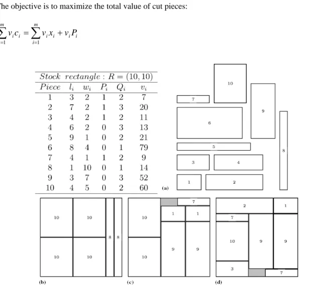
In the two-dimensional non-guillotine cutting problem, we consider a large stock rectangle R = (L, W) of length L and width W. We also consider m types of small pieces. Each type of piece i (i =1,...,m) is characterized by its dimensions li, wi

0

<

l

≤

L

,

0

<

w

≤

W

Each type of piece i may also have ci copies such that

P

≤

c

≤

Q

(

i

=

1

,

K

m

)

minimum and the maximum number of copies of type i.

The set of pieces to cut has to be determined in order to respect the minimum constraints Pi (i

=1,…, m). That is why we define the variables xi(i =1,..., m) which represent the number of copies

of type i cut in excess of the lower bound Pi :

i i

i

c

P

x

=

−

i

=

1

,...,

m

The objective is to maximize the total value of cut pieces:

i i m

i

m

i i i i

i

c

v

x

v

P

v

=

+

∑

∑

=1 =1

(2)

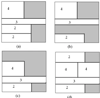
Figure 1. Instance 3 from Beasley (b) Unconstrained optimal solution (c) Constrained optimal solution (d) Doubly constrained optimal solution

Depending on the values of Pi and Qi we distinguish three types of problems:

– Unconstrained:

∀

i

=

1

,...,

m

,

P

=

0

,

Q

=

⎣

L

×

W

/(

l

×

w

)

⎦

– Constrained:

∀

i

=

1

,...,

m

,

P

=

0

,

∃

1

≤

i

≤

m

,

Q

<

⎣

L

×

W

/(

l

×

w

)

⎦

– Doubly constrained: ∃1≤i≤m,

P

>

0

,

∃

1

≤

j

≤

m

,

Q

<

⎣

L

×

W

/

l

×

w

⎦

In function of the considered problem, the optimal solution is different as illustrated by the example of Figure1, cited in Alvarez-Valdes et al. (2005).

Let ei be the efficiency of a piece i =1,...,m such that ei = vi/(li × wi). According to this definition, we

distinguish two types of problems:

– Unweighted:

e

=

1

∀

i

=

1

,...,

m

– Weighted:

e

≠

1

∀

i

=

1

,...,

m

2.2. Literature Review

As mentioned above, as far as we are concerned, we are interested by the constrained problem. The unconstrained version has been already treated by Tsai et al. (1998), and by Healy et al. (1999). For the constrained problem, some exact methods have been proposed in the literature. Beasley (1985) was the first to propose an exact branch and bound algorithm where the upper bound was derived from Lagrangian relaxation of a (0-1) integer programming formulation of the problem. More research has been conducted by Scheithauer and Terno (1993), Hadjiconstantinou and Christofides (1995), Fekete and Schepers (1997), and Caprara and Monaci (2004).

Alvarez-Valdes et al. (2005, 2007) proposed a simple upper bound. This bound is obtained by solving the following bounded knapsack problem, where variables xi represent the number of pieces

of type i to be cut in excess of its lower bound Pi.

max

∑

∑

= =

+

i

x

v

P

v

1 1

:

.

.

t

s

∑

∑

= =

−

×

≤

i

w

x

L

W

P

l

w

l

)

(

)

(

,

i

Q

P

x

≤

−

i

=

1

,...,

m

,

0

≥

i

x

i

=

1

,...,

m

Other bounds included in exact methods, as mentioned above, were proposed by Scheithauer and Terno (1993) and recently by Hadjiconstantinou et al. (2002), who developed a new upper bound based on an integer programming model. This model handles capacity constraint, the non-overlapping constraint, uniqueness of placement and a position constraint.

Heuristic methods were proposed by Biro and Boros (1984), Farley (1999) and recently by Wu et al. (2002) who developed a constructive algorithm when Pi= Qi, i =1,..., m. In their approach, a piece is cut in the corner of the current cutting pattern and the choice of piece to be cut is selected according to a fitness evaluation function.

Several metaheuristics are available. Lai and Chan (1997) and Leung et al. (2001) proposed simulated annealing and genetic algorithms. Alvarez-Valdes et al. (2005) developed a GRASP algorithm which is based on a constructive algorithm. We also use this constructive algorithm in this work (algorithm 2). They investigated several strategies for the improvement phase and several choices for critical search parameters. The computational results show that their idea is suitable for Beasley’s constrained and doubly constrained test problems. Alvarez-Valdes (2007) applied a Tabu search for the same problem, with two moves, based on the reduction and insertion of blocks of pieces. The efficiency of the moves is based on merging the empty rectangles and filling with the pieces still to be cut. Intensification and diversification strategies based on long term memory are included. This method gives very good results for constrained test problems.

3. ADAPTATION OF ITERATED LOCAL SEARCH METHOD

In this section, the ILS approach is adapted to our problem. First, we give the definition of an ILS algorithm, and then we present the three procedures which are used.

3.1 Iterated Local Search (ILS)

According to Glover et al. (2002), Iterated Local Search (ILS) is a simple and generally applicable stochastic local search method that iteratively applies local search to perturbations of the current search point, leading to a randomized walk in the space of local optima. The ILS algorithm starts from a local optimal solution obtained by the local search algorithm and, and at each iteration, a copy of the current solution is perturbed and improved by the local search. If the new solution is better than the current one, the next iteration starts with the new solution, otherwise the current solution is perturbed again.

ILS is based on a deterministic heuristic which is used to generate the starting point solution. Perturbation is used to generate new starting points for the local search. To apply ILS we define three procedures: the constructive heuristic, the perturbation procedure and the local search one. These three procedures use the placement algorithm, which is used to decide how to place a piece in the empty space before cutting it.

3.2. Placement Procedure

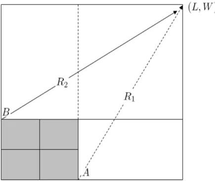
Let n be the number of copies not yet cut for one given piece and b a block of these n copies, arranged in rows and columns, such that the number of copies in the block does not exceed Qi. We want to place this block in the empty space of the large rectangle, using the concept of empty rectangle. We define an empty rectangle as a rectangle that contains no blocks. It is determined by its free point. A free point is a corner of an already placed block. For example, in Figure 2, we have a block of four copies placed in the lower left corner of the large rectangle. The free points generated by this block are:

– A: the lower right corner of the block. – B: the upper left corner of the block.

Figure 2. Placement procedure

By placing the block of four copies, two rectangles are created. The empty rectangle R1 is

characterized by its free point A which correspond to the bottom left corner and by its upper right corner of coordinates (L, W). The empty rectangle R2 is characterized by its free point B which

correspond to the bottom left corner and by its upper right corner of coordinates (L, W).

The Algorithm 1 presents the placement procedure which is used in the constructive algorithm in order to place the blocks in the large stock rectangle. In this procedure each block is placed nearest the corners (bottom left, bottom right, upper right and upper left) of the large rectangle such that: – its bottom edge touches either the bottom of the large rectangle or the top edge of another block and its left edge touches either the left edge of the large rectangle or the right edge of another block for bottom left position.

– its bottom edge touches either the bottom of the large rectangle or the top edge of another item and its left edge touches either the right edge of the large rectangle or left edge of another block for bottom right position.

– its top edge touches either the top of the large rectangle or the bottom edge of another block, and its left edge touches either the left edge of the large rectangle or the right edge of another block for upper left position.

– its top edge touches either the top of the large rectangle or the bottom edge of another block, and its left edge touching either the right edge of the large rectangle or the left edge of another block for upper right position.

Once a block is placed in a position in the large rectangle, we update the list of empty rectangles by removing the used rectangle and create new rectangles generated by the free points of the already placed block and by modifying the empty rectangles dimensions in order to avoid overlaps.

Algorithm 1 – Placement procedure for one given block

1: ifb can fit in the first rectangle of the list in lower left corner then

2: Place b in this position

3: Update the list of empty rectangles according to the free points and their dimensions. 4: else ifb can fit in the first rectangle of the list in lower right corner then

5: Place b in this position

6: Update the list of empty rectangles according to the free points and their dimensions. 7: else ifb can fit in the first rectangle of the list in upper left corner then

8: Place b in this position

9: Update the list of empty rectangles according to the free points and their dimensions. 10: else ifb can fit in the first rectangle of the list in upper right corner then

11: Place b in this position

12: Update the list of empty rectangles according to the free points and their dimensions. 13: end if

3.3. The Constructive Heuristic

We use the constructive algorithm of Alvarez-Valdes et al. (2005) described in Algorithm 2. This heuristic is an iterative process. At each iteration, a piece is chosen to be cut. The process is stopped if no piece can be cut. Consider a set PC of type pieces, where each type i =1,...,m, is characterized by its dimensions (li,wi), its value vi and lower bound Pi. Define a set Q where Qi is the upper bound

on the number of copies of type i (i =1,...,m) still to be cut. We also define a set C, where Ci is the

number of cut copies of type i (i =1,...,m).

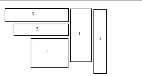
Consider an example (Instance 1 from Beasley (2004)) in Figure 3. We apply the constructive algorithm. In this example we have 5 types of pieces (m = 5).

Piece li wi Pi Qi vi ei

1 3 7 0 2 35 1.66

2 8 2 0 2 40 2.5

3 10 2 0 1 27 1.35

4 5 4 0 3 23 1.15

Algorithm 2 – Constructive algorithm of Alvarez-Valdes et al. 1: Initialize

2: The list of empty rectangles is initialized by the large stock rectangle R = (L, W ). – PC={pc1, pc2, . . . , pcm}.

– Q = {Q1,Q2,...,Qm}.

– C =Ø.

3: Order the type pieces of PC according to 3 criteria:

(a) Order by Pi × li× wi non-increasing giving priority to pieces which must be cut.

(b) Break ties by non-increasing ei.

(c) Break remaining ties by non-increasing li × wi.

4: In the PC order, find the first index j (such that Qj> 0) of type piece which can fit in the

stock rectangle. If it does not exist, stop; else go to step 4.

5: Find the maximum value

0

<

n

≤

Q

6: Call the placement procedure to place the block b. 7: Update Q : Qj = Qj - n, Cj= Cj+ n, go to step 3.

Figure 3. Instance 1 from Beasley

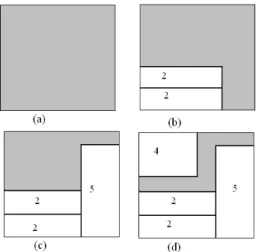
Initially PC = {2, 5, 1, 3, 4} in the efficiency order and Q = {2, 2, 2, 1, 3}. We consider the first piece in the list (piece 2) with Q2 =2, we cut it twice in the lower left corner of the large stock

rectangle. We update Q = {0, 2, 1, 3, 2} and C = {0, 2, 0, 0, 0} (see (b) in Figure 4). We try to cut a piece 5 with Q5 =2, but only one piece can fit in the empty space. We place this piece in the lower

right corner (see (c) in Figure 4). We update Q = {0, 2, 1, 3, 1} and C = {0, 2, 0, 0, 1}, then we consider the pieces 1, 3 but they do not fit into the empty space of the large rectangle.

We take the last piece in PC, piece 4 with Q4 =3, and cut a block with one copy at the upper left

Figure 4. Instance 1 Beasley (1985). Selecting the most efficient piece.

3.4. The Perturbation Procedure

The perturbation procedure described in Algorithm 3 consists in a permutation between cut and uncut pieces in random order. The aim of this procedure is to generate new starting points for the local search. Consider PC and PC the sets of type of pieces still to be cut and C, C the sets of cut pieces. The algorithm 3 presents this procedure.

Algorithm 3 – Perturbation procedure 1: C=C

2: repeat

3: Draw randomly p_i∈C 4: Remove pi from the solution.

5: PC =PC 6: repeat

7: Draw randomly p_k ∈PC

8: Try to cut pk with the placement procedure.

9: if failure then

10: PC =PC\{pk}

11: end if

12: until PC= Ø or permutation done 13: if PC= Ø then

14: C =C\{pi}

15: Put pi back in the solution.

16: end if

For example, in Instance 1 from Beasley (2004), we swap piece 5 and piece 3. The new solution is presented in Figure 5:

Figure 5. Instance 1 from Beasley (1985). Permutation between pieces 5 and 3.

3.5. The Local Search Procedure

We tested several local search procedures in order to find the best one. The first one consists in eliminating the final k% blocks of the solution (the last 10%). Once the final pieces have been removed from the solution, the constructive algorithm is applied. Preliminary tests have shown that give poor results, even using different values for the parameter k.

Figure 6. Instance 1 Beasley (1985). (a) perturbed solution. (b) solution after removing piece 2. (c) moving to the corners. (d) fill.

For this reason, we tested another method which consists in removing cut pieces in random order and moves the remaining ones to the corners of the large rectangle and finally filling the empty space by applying the constructive algorithm. When selecting the piece to cut, the piece eliminated is not considered until another piece has been included in the modified solution.

For the same previous example (Instance 1 from Beasley (2004)), we applies the local search to the configuration obtained after the perturbation in Figure 5. Randomly, we decide to remove piece 2

and we get the Figure 6 (b). Then, we move the remaining pieces to the corners of the large rectangle (Figure 6 (c)) and apply the constructive algorithm which leads to the configuration in Figure 6 (d).

3.6. General Structure of the ILS Algorithm

We present in Algorithm 4 the general structure of the ILS algorithm. BestSol, denotes the best solution and BestValue the value of the best solution. Sol is a solution characterized by the set C of cut copies of pieces. Value is the value of the solution sol and MaxIterations is the number of iterations.

Algorithm 4 – General structure of the ILS 1: BestSol = solution of constructive algorithm 2: BestValue =

∑

bestsol

C

i

v

x

3: Sol = Local search (BestSol) 4: Value =

∑

∈Csol

i i ix v

5: if Value > BestValue then 6: BestSol = Sol

7: BestValue = Value 8: end if

9: for count =1 to MaxIterations do 10: Sol = BestSol

11: Sol = Perturbation (Sol) 12: Sol = Localsearch (Sol) 13: Value =

∑

∈Csol

i i ix v

14: ifValue > BestValuethen 15: BestSol = Sol

16: BestValue = Value 17: end if

18:end for

4. COMPUTATIONAL RESULTS

To test our approach, we have used several sets of test problems:

– A set of 21 problems from literature: 12 from Beasley (2004), 2 from Hadjiconstantinou and Christofides (1995), 1 from Wang (2003),1 from Christofides and Whitlock (1977) and 5 from Fekete and Schepers (1997). The length and width of the large rectangle vary in [10, 100], the number of pieces in [5, 30] and the maximum number of pieces which could be cut in [10, 97]. For all of them, the optimal solutions are known.

– A set of 10 problems from Leung et al. (2003), consisting of 3instances from Lai and Chan (1997), 5 from Jakobs (1996) and 2 from Leung et al. (2003). The length and width of the large rectangle vary in [45, 400], the number of pieces in [5, 50] and the maximum number of pieces which could be cut in [10, 50].

– A set of 630 large problems generated by Beasley (2004). All the problems have a stock rectangle of size (100, 100). According to Alvarez-Valdes (2005, 2007), for each number of piece types m (m =40, 50, 100, 150, 250, 500, 1000), 10 problems are randomly generated with Pi=0, Qi

= 1;3;4 for i=1,...,m. These 630 instances are divided into 3 types, according to the percentages of the types of pieces of each class (Table 1, Table 2):

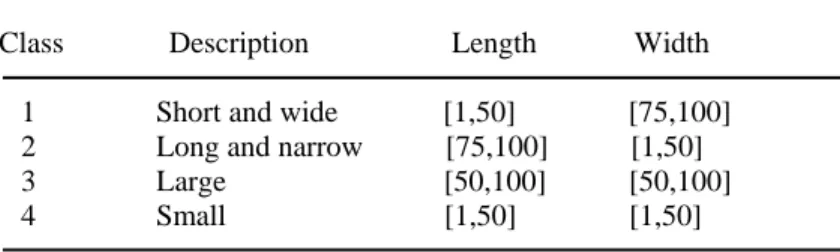
Table 1. Length and width for each class

Class Description Length Width 1 Short and wide [1,50] [75,100] 2 Long and narrow [75,100] [1,50] 3 Large [50,100] [50,100] 4 Small [1,50] [1,50]

Table 2. Percentage of pieces of each class Type Class

1 2 3 4 1 20 20 20 40 2 15 15 15 55 3 10 10 10 70

The value assigned to each piece is equal to its area multiplied by an integer randomly chosen from {1,2,3}.

– A set of Hopper and Turton (2001) instances in which each piece appears once (Q =1) and its value is equal to its area. The length and width of the large rectangle vary in [20, 240].

4.1. Implementation

Our ILS has been coded in Delphi 7 and run on a 2.8 GHz Pentium 4. The algorithm runs until it reaches the optimal solution, if known, or the corresponding upper bound, or after 500 iterations. The complete computational results appear in the following tables. The four tables include a direct comparison with the GRASP algorithm and Tabu search algorithm of Alvarez-Valdes (2005, 2007). In these tables MPDO indicates the Mean Percentage Deviation from Optimum and NOS the Number of Optimal Solutions. In Tables 3, 4 and 6, the ILS values are compared with the optimal solutions (Beasley (2004)) and with the GRASP algorithm and Tabu search results (Alvarez-Valdes (2005, 2007)). For the large instances in Table 5 the optimal solutions are unknown, the comparisons are made with the upper bounds obtained by solving the knapsack problem presented in section 2.2. In this table we calculate the percentage of deviation from the upper bounds which we indicate by MPDUP.

Table 3. Instances from literature

Instances L, H m GRASP CPU

Time

Tabu CPU Time Optimum ILS CPU Time

10;10 5 164 0 164 0,06 164 164 0

Beasley 10;10 7 230 0 230 0 230 230 0

10;10 10 247 0 247 0 247 247 0,09

15;10 5 268 0 268 0 268 268 0

15;10 7 358 0 358 0 358 358 0

15;10 10 289 0 289 0 289 289 0

20;20 5 430 0 430 0 430 430 0

20;20 7 834 0,77 834 0,16 834 834 0,52

30;30 10 924 0 924 0,05 924 924 0,23

30;30 5 1452 0 1452 0 1452 1452 0

30;30 7 1688 0,05 1688 0,06 1688 1688 0,32

30;30 10 1865 0,05 1865 0 1865 1865 0,61

Hadjiconstantinou 30;30 7 1178 0 1178 0 1178 1178 0

and Christofides 30;30 15 1270 0 1270 0,11 1270 1270 0

Wang 70;40 19 2726 0,77 2726 0,06 2726 2726 1,82

Christofides and Whitlock

40;70 20 1860 0,39 1860 0,05 1860 1860 0,16

Fekete and 100;100 15 27589 2,31 27718 2,14 27718 27698 1,95

Schepers 100;100 30 21976 4,17 22502 3,4 22502 21844 4,98

100;100 30 23743 3,68 24019 0,66 24019 23952 1,39

100;100 33 32893 0 32893 0 32893 32893 0

100;100 29 27923 0 27923 0 27923 27923 0

MPDO 0,19% 0,58 0% 0,32 0 0,15% 0,57

NOS 18 21 21 18

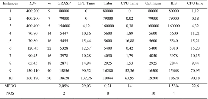
Table. 4. Instances from Leung et al. (2003)

Instances L;W m GRASP CPU Time Tabu CPU Time Optimum ILS CPU time

1 400;200 9 80000 0 80000 0 80000 80000 1,12

2 400;200 7 79000 0 79000 0,02 79000 79000 0,18

3 400;400 5 154600 4,12 160000 0,38 160000 160000 4,32

4 70;80 14 5447 10,16 5600 1,89 5600 5600 11,21

5 70;80 16 5455 15,44 5600 16,88 5600 5540 15,21

6 120;45 22 5328 12,57 5400 0,42 5400 5310 15,23

7 90;45 16 3978 10,28 4050 1,79 4050 3978 10,15

8 65;45 18 2871 14,94 2925 1,53 2925 2844 9,44

9 150;110 40 15856 90,52 16280 52,36 16500 15668 70,95

10 160;120 50 18628 132,26 19044 63,95 19200 18628 90,18

MPDO 2,05% 29,03 0,21 14 1,53% 22,6

Table 5. Larger instances

m Q M = m × Q GRASP CPU time Tabu CPU time ILS CPU time 40 1 40 6,97 2,33 6,55 10,97 6,89 2,38

3 120 2,22 6,62 1,95 14,2 1,78 5,88 4 160 1,81 4,44 1,65 18,26 1,8 4,02

50 1 50 4,8 4,71 4,85 15,26 4,8 3,33

3 150 1,5 7,05 1,27 22,5 1,23 8,06

4 200 1,18 5,34 0,96 18,19 1,09 6,02

100 1 100 1,51 5,36 1,5 38,79 1,51 9,2

3 300 0,47 9,41 0,31 32,11 0,5 10

4 400 0,26 6,99 0,18 19,67 0,23 14,12 150 1 150 0,89 5,53 0,07 54,9 0,88 11

3 400 0,14 11,71 0,05 31,76 0,11 18,03 4 600 0,11 6,75 0,45 19,67 0,09 20,74 250 1 250 0,51 5,27 0,01 90,07 0,51 14,31

3 750 0,04 13,89 0 13,7 0,04 13,8

4 1000 0,03 6,65 0 4,5 0 5,75

500 1 500 0,05 3,24 0,03 86,17 0,055 4,1

3 1500 0 12,24 0 1,1 0,01 8,4

4 2000 0 1,15 0 0,84 0 1,09 1000 1 1000 0 1,01 0 7,8 0 0,18

3 3000 0 6,53 0 1,54 0,02 4,23

4 4000 0 0,29 0 1,19 0 1,12 MPDUP 1,07 6,01 0,97 25,34 1,03 7,89

For the first set of 21 instances (Table 3), the average distance to optimum is 0.15% compared to 0.19% for the GRASP. We improve two instances and do as well as GRASP for 18 others. We obtain 0.57s of execution time versus 0.58s for the GRASP and 0.32s for Tabu search. For the

second set (Table 4), ILS outperforms the GRASP for 3 instances and does as well as the GRASP and the Tabu search for 4 instances. The mean percentage of deviation from the optimum is 1.53% versus 2.05% for the GRASP and 0.21% for the Tabu search.

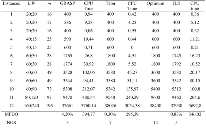
Table 6. Instances from Hopper and Turton (2001)

Instances L;W m GRASP CPU Time

Tabu CPU Time

Optimum ILS CPU time

1 20;20 16 400 0,94 400 0,42 400 400 0,36

2 20;20 17 386 9,28 400 4,23 400 400 5,12

3 20;20 16 400 0,06 400 0,95 400 400 0,32

4 40;15 25 590 19,44 600 0,44 600 600 11,21

5 40;15 25 600 0,71 600 0 600 600 0,21

6 60;30 28 1765 26,8 1800 4,91 1800 1745 16,23 7 60;30 28 1774 30,92 1800 5,52 1800 1792 10,52 8 60;60 49 3528 102,05 3580 45,27 3600 3580 20,17 9 60;60 49 3544 94,41 3580 51,11 3600 3542 80,15 10 60;90 73 5308 212,07 5342 135,97 5400 5312 100,8 11 80;120 97 9470 480,44 9548 240,39 9600 9460 204,6 12 160;240 196 37661 3760,14 38026 3054,38 38400 37930 3692,8 MPDO 4,20% 394,77 0,30% 295,39 0,83% 346,02

NOS 3 7 12 5

The average execution time is 22.6s compared to 29.03s for the GRASP. For the larger instances, (Table 5) shows that the average deviation from the knapsack upper bound is 1.03% compared to 1.07% for the GRASP and 0.97% for the Tabu search. We outperforms the GRASP for 11 subsets (for (m= 50, Q= 1, 3, 4); (m=50, Q= 3, 4); (m=100, Q=4); (m=150, Q=1, 3, 4); (m=250, Q=3, 4)) and find the same results for 7 others. ILS supersedes the Tabu search for the second subset which corresponds to (m=40, Q=3). The average distance from the knapsack upper bounds is 1.78% for ILS compared to 1.95% for the Tabu search. For the subset (m=50, Q=1) the mean percentage of deviation from knapsack upper bounds is 4.80% for ILS versus 4.85% for Tabu search. The average distance of the knapsack upper bounds for the subset (m=50, Q=2) is 1.23% for ILS versus 1.27% for the Tabu search and the subset (m=150, Q=4) the mean percentage of deviation from knapsack upper bounds is 0.09% compared to 0.45% for the Tabu search. However ILS does as well as the Tabu search for 4 subsets which correspond to (m=250, Q=4), (m=500, Q=4) and (m=1000, Q=1, 4).

For the instances of Hopper and Turton (2001) we note that the average distance to the optimum is 0.83% compared to 4.20% for the GRASP. We improve 7 instances and do as well as the GRASP for 3 others. ILS also supersedes the Tabu search for one instance and achieves the same results for 6 others.

5. CONCLUSION

We have presented an Iterated Local Search for the constrained two-dimensional non-guillotine cutting problem, which is based on three procedures: a constructive algorithm used to generate the starting points, a perturbation procedure which consists in permutation between cut and uncut pieces, and a local search which removes cut pieces. The computational results are very competitive compared to the GRASP of Alvarez-Valdes (2005). In the first set the average distance to the optimum is 0.15% compared to 0.19% for the GRASP. For the second set the mean percentage of deviation from optimum is 1.53% versus 2.05% for the GRASP. For the larger instances the average deviation from the knapsack upper bounds is 1.03% compared to 1.07% for the GRASP. Finally, for the last set (Hopper and Turton (2001) instances), the average deviation from the optimum is 0.83% compared to 4.20% for the GRASP. ILS outperforms the Tabu search for some instances of the larger instances and for some instances of Hopper and Turton (2001). To improve the results, we suggest adding other moves in the local search and combining this method with the GRASP algorithm.

ACKNOWLEDGMENTS

This work has been supported in part by Champagne Ardenne Regional Council and the European Social Fund.

REFERENCES

[1] Alvarez-Valdes R., Parreno F., Tamarit J.M. (2005), A Grasp algorithm for constrained two-dimensional non guillotine cutting problems; Journal of Operational Research Society 56(4); 414-425. [2] Alvarez-Valdes R., Parreno F., Tamarit J.M. (2007), A Tabu search algorithm for two-dimensional non

guillotine cutting problems; Journal of Operationan Research 183; 1167-1182.

[3] Beasley J.E. (1985), A two dimensional non guillotine cutting tree search procedure; Operations Research 33(1); 49-64.

[4] Beasley J.E. (2004), A population heuristic for constrained two-dimensional non-guillotine cutting problems; European Journal of Operational Research 156(3); 601-627.

[5] Biro M., Boros E. (1984), Network flows and non-guillotine cutting pattern; European Journal of Operational Research 16; 215-221.

[6] Caprara A., Monaci M. (2004), On the two-dimensional Knapsack problem; Operations Research Letters 32; 5-14.

[7] Christofides N., Whitlock C. (1977), An algorithm for two dimensional cutting problems; Operations Research 25; 30-44.

[8] Farley A.A. (1999), Selection of stock plate characteristics and cutting style for two dimensional cutting stock situations; European Journal of Operational Research 44; 239-246.

[9] Fekete S.P., Schepers J. (1997), On more-dimensional packing III: Exact Algorithms, Report No.97.290; Technical University Berlin.

[10] Garey M.R., Johnson D.S. (1979), Computer and intractability: A guide to the theory of NP-completeness; Freeman and Company; San Francisco.

[11] Glover F., Kochenberger G. (2002), Editors, Handbook of metaheuristics; International series in operations research and management science vol. 57; Kluwer Academic Publishers, Norwell, MA, 321-353.

[12] Hadjiconstantinou E., Boschetti M.A., Mingozzi A. (2002), New upper bounds for the two-dimensional orthogonal non-guillotine cutting stock problem; IMA Journal of Management Mathematics 13; 95-119.

[13] Hadjiconstantinou E., Christofides N. (1995), An exact algorithm for general orthogonal two-dimensional knapsack problems; European Journal of Operational Research 83; 39-56.

[14] Healy P., Creavin M., Kuusik A. (1999), An optimal algorithm for placement rectangle; Operations Research Letters 24; 73-80.

[15] Hopper E., Turton B.C.H. (2001), An empirical investigation of meta-heuristic and heuristic algorithms for a 2D packing problem; European Journal of Operational Research 128; 34-57.

[16] Jakobs S. (1996), On genetic algorithms for the packing of polygons; European Journal of Operational Research 88; 165-181.

[17] Lai K.K., Chan J.W.M. (1997), Developing a simulated annealing algorithm for the cutting stock problem; Computers and Industrial Engineering 32; 115-127.

[18] Leung T.W., Yung C.H., Troutt M.D. (2001), Applications of genetic search and simulated annealing to the two-dimensional orthogonal packing problem; Computers and Industrial Engineering 40; 201-214.

[19] Leung T.W., Yung C.H., Troutt M.D. (2003), Application of a mixed simulated annealing-genetic algorithm heuristic for the two-dimensional orthogonal packing problem; European Journal of Operational Research 145; 530-542.

[20] Scheithauer G., Terno J. (1993), Modeling of packing problems; Optimization 28; 63-84.

[21] Tsai R.D., Malstrom E.M., Meeks H.D. (1988), A two-dimensional palletizing procedure for warehouse loading operations; IIE Transactions 20; 418-425.

[22] Wächer G., Haussner H., Schumann H. (2007), An improved typology of cutting and packing problems; European Journal of Operational Research 183; 1109-1130.

[23] Wang P.Y. (2003), Two algorithms for constrained two-dimensional cutting stock problems; Operations Research 31; 573-586.

[24] Wu Y.L., Huang W., Wong S.C., Young G.H. (2002), An effective quasi-human based heuristic for solving rectangle packing; European Journal of Operational Research 141; 341-358.