Journal of Industrial and Systems Engineering Vol. 8, No. 3, pp 24-41
Summer 2015
Two new heuristic algorithms for covering Tour Problem
Mehdi Alinaghian
1*, AlirezaGoli
21,2Department of Industrial and Systems Engineering, Isfahan University of Technology,
Isfahan, Iran
[email protected], [email protected]
Abstract
Covering tour problem (CTP) is the generalized form of Traveling Salesman Problem (TSP), which has found different applications in the designing of distribution networks, disaster relief, and transportation routing. The purpose of this problem is to determine the Hamiltonian cycle with the lowest cost using a subset of all the nodes, such that the other nodes would be in a distance shorter than the pre-specified one, from at least one visited node. In this paper, two new heuristic algorithms called MDMC (minimum distance-maximum covering) and AGENI (adapted generalized insertion) are presented to solve CTP. In order to assess the performance of the proposed algorithms in small scale, several test problems are accurately solved and the results are compared with those from the proposed heuristic algorithms. Also, in large scales, the results of each of proposed algorithms are compared with the three heuristic algorithms, existing in the literature. Finally, the effect of neighborhood searches on the performance of the proposed algorithms will be investigated. The results show that the performance of the proposed algorithms in small and large scale test problems used in this paper is appropriate.
Keywords: covering tour problem; local search; heuristic methods.
1- Introduction
Covering problem was introduced for the first time in 1964 (Schilling, Jayaraman and Barkhi, 1994). In this problem, service presentation depends on the distance between customer and facilities. In this problem, a customer can receive service from a facility when the distance between the customer and one of the facilities, is shorter than or equal to the covering distance (covering criterion). Covering distance is the radius of the area, within which if a customer is located, she/he will be able to receive service from the facility or be covered by it. Covering distance can be defined as time or cost. Covering problem is divided into two covering types of full coverage and partial coverage in terms of the coverage of points (Daskin, 1995).
Covering tour problem (CTP), is a form of the general covering problem in which, the facilities of the service provider, are in the travelling points of a vehicle, or in other words, the vehicle is tasked with responding to customer demands. CTP is defined on theG=(V ∪W E, )graph, in which,
1 2
{ ,
,...,
n}
V
=
v v
v
is the set of the nodes which a vehicle can travel through, andT
⊆
V
, are the*Corresponding author.
nodes which the vehicle must travel through.The starting point of (
v
1) vehicle, is described as the depot andv
1∈
T
. The set of the nodes that must be covered are presented byW
=
{
w w
1,
2,...,
w
m}
. Also E={(v vi, j) :v vi, j∈ ∪V W}describes the edges or communication paths between different points of a network.To demonstrate demand point’s coverage, covering matrix A=[aij]mnwith the covering distance ofτ
are used, defined in equation 1.The density function of
ρ
covering matrix, as shown in equation 2, is a criterion to show the coverage level of theW
set. The bigger this criterion is, the closer the network nodes together and the larger the covered area will be.The purpose of this problem is to determine the travelling points of a vehicle, or in other words, to determine the traveling tour of the vehicle such that all the
W
points are covered and the length of the formed tour is minimized (Hodgson, Laporte and Semet, 1998).Different types of CTP have been introduced, and the following ones can be mentioned as examples.
• Tour multiplicity for vehicle: in this type, a vehicle returns to depot after finishing its tour and starts another tour. This type is applicable when the number of covered nodes and the nodes that can be visited is high and only one vehicle is available. In addition some limitations such as maximum travelling time or capacity exist.
• Vehicle multiplicity: A number of vehicles are available and each of them has an individual tour.
• Depot multiplicity: A number of depots exist in networks and each vehicle has started its travel from one of the depots to which or to another depot, it returns at the end.
• Covering tour along with demand and limited vehicle capacity: Covered nodes, each have a certain demand of one or more goods, and the vehicle with limited capacity for carrying the required goods, is tasked with providing a part or all of this demand.
In continue, in the section 2 of the paper, the CTP literature is reviewed. In section 3, the mathematical model of the problem is presented. In section 4, Heuristic methods to solve CTP are introduced. Numerical results are presented in section 5 and finally conclusion is presented in section6.
1
0
ij ij
if e
if e
τ
τ
≤
>
1,2,..., 1,2,...,
i m
j n
= =
ij a
)
1
(
)
2
(
1 1
m n ij i j
a mn
2- CTP literature and similar problems
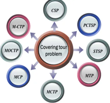
CTP has many similar problems, some of which are shown in figure 1.
Figure 1. CTP-related problems
CTP can be introduced as an example of TSP, in which the assumption of visiting all cities doesn't exist (Salari and Naji-Azimi, 2012). This problem is very similar to covering salesman problem (CSP), but in CSP, all the groups are of one type and their starting points can be any of a graph's nodes.
CSP is recognized with the purpose of selecting a tour with the lowest cost such that the P cities are travelled through and other cities would be located in the covering distance of the visited cities. The difference between this problem and CTP is in the structure of the problem's network. Current & Schilling (1989) used CSP to select paths for disaster relief for cities. They selected the visited cities in a way that other cities, would be located very near to them, and the people in these cities who had demands, would be able to walk to the visited cities and receive disaster relief. They presented an integer linear model for their problem and extracted the best possible response with a 2-stage heuristic algorithm, based on the sets' coverage.
Arkin and Hassin (1994) introduced CSP by considering geometric distance. They considered the travelling path of the salesman in a continuous space and calculated the distances between the points as Euclidian distances. Their aim was to minimize the total distance travelled by salesman who starts moving from one point, and after finishing its Hamiltonian cycle, returns back to the same point. They implemented their model by some simple heuristic algorithms.
Current and Schilling (1994) introduced two bi-criteria models for CSP and called them median tour problem (MTP) and maximal covering tour problem (MCTP). In both of the problems, the tour should include the p cities and the length of the tour should be minimized. In MTP, the second goal is to minimize the distance between the visited and unvisited cities. In MCTP, the second goal is to maximize the satisfied demand from the visited cities and their covered cities.
Gendreau, Hertz and Laporte (1992) considered CTP in a special form, that the nodes would include two groups. W1 is a group of nodes which can be visited, and W2 is the set of the nodes that must be
covered. The aim of their model, is to minimize the Hamiltonian cycle length among the W1nodes,
such that all the W2nodes would be covered. To solve this problem, they first presented a branch and
can be visited (W1). Also, using the algorithm offered by Current and Schilling (1994), they offered
the best possible responses for their model.
Hachicha et al (2000), introduced the multi-vehicle covering tour problem (m-CTP).They considered the nodes in two types, one type that can be visited and the other that is covered, and wanted to minimize the distance travelled by each vehicle. All of these vehicles deliver one desired item to their own transit points concerning the other assumptions of this problem as follows.
• Each vehicle starts to move from one depot and returns again to it.
• Only one vehicle passes through each point.
• The number of the nodes passed by each vehicle can at most be equal to the constant number of p.
• The length of the tour of each vehicle cannot be more than the constant value of q.
Golden et al (2012), offered two heuristic methods for the CTP model presented by Current and Schilling, and called them LS1 and LS2. LS1, aims to improve a selected tour in two stages. In the first stage, it increases and decreases the number of the visited cities, and in the second stage, it investigates the reasonability of a selected tour. LS2 specifies the best possible cycle according to the cities selected for visiting with the use of Lin and Kernigan's algorithm (Lin and Kernighan, 1973). At the end, using these two heuristic methods, it tries to escape from local optimal point and find a general optimal response.
Salari and Azimi (2012) introduced a linear integer model which is based on local search for CSP. In their assumed network only one type of node exists and the transit points can be any of the network point’s .The goal is to minimize the tour length and the coverage of all the network nodes. Their offered model can be used for similar problems such as CTP.
CTP is also related to prize-collecting traveling salesman problem (PCTSP) and selective travelling salesman problem (STSP). In each of these problems, for each i node, there's a non-negative profit equal to pi. In PCTSP, the goal is to minimize the length of the selected tour among some nodes, such
that the minimum expected profit would be gained. This model was introduced for the first time by Fischetti and Toth (1988). On the opposite, in STSP, the goal is to maximize the profit gained from tour selection for travelling, such that the tour length would not exceed the maximum allowable length. This problem was introduced for the first time by Laporte and Matrello (1990). In both of the above cases, the problem is formulated using an integer linear programming approach, and with the branch and bound algorithm, its optimal response for a number of nodes of less than or equal to 100, was obtained.
Another type of relevant problem, is median cycle problem (MCP). This problem has two types. In the first type which is called MCP1, the goal is to minimize the length of the selected cycle and the distance between the visited and unvisited points. This problem was introduced for the first time by Labbé et al (2004). Another type of this problem known as MCP2, has minimized cycle length, while there's an upper bound limitation for the distance between visited and unvisited points. Pérez, Moreno and Martı́n (2003) introduced the two similar problems and an integer linear model for each of them. Another type of relevant problem is bi-objective covering tour problem (BOCTP). Jozefowiez, Semet and Talbi (2007) introduced and investigated this problem. They aimed to minimize the tour of vehicle while minimizing the maximum distance of covered point. The network of study has two types of nodes. One type are the nodes that can be visited, some of which must certainly be visited, and another type of nodes, which must be covered. They showed that each response to this problem has two parts. The first part, is related to set covering problem (SCP) and the second part is related to TSP.
Another type of BOCTP is offered in the researches of Tricoire , Graf and Gutjahr (2012). They investigated CTP with fuzzy demand. Their problem, aims to specify some points in network to establish distribution center for critical conditions and vehicle routing between these distribution centers. In this research, the location of distribution centers are selected in a way that the other network points would be placed in the distance covered from distribution centers. They offered a bi-objective model for this area. In its first goal, the sum of the implementation costs of distribution centers and goods transportation by vehicle are minimized, and in the second goal, the uncovered demand, is minimized.
Multi-objective covering tour problem (MOCTP) was introduced for the first time by Nolz et al (2010) in which some vehicles start to move from a central depot and after visiting some nodes, they return to the same depot. Each node has a specific demand which must be satisfied by a vehicle. The goal of this problem is to minimize the functions below:
1- Linear combination of the distances between all the nodes with the nearest visited node and the number of the nodes with no access to the visited node.
2- Total distance travelled by vehicles.
3- Maximum distance travelled per each vehicle.
These researchers presented bi-objective models. At first, they minimized the first and second objective functions, and then they minimized the first and third functions. For each of these conditions, neighborhood searches are developed based on genetic algorithm and efficient responses are offered from these models.
Jozefowiez (2014) introduced a mathematical model and a branch and bound algorithm to solve MCTP. This researcher considered the importance level of different covered points and defined individual weights for each covered point. At the end, using random numerical examples, the accuracy of the solution method was investigated.
Azimi and Salari (2014) added time limit to CSP. Also, they changed the objective function of this problem to the maximization of the number of covered points. In this regard, these researchers offered a new mathematical model and some heuristic methods and compared them with recent heuristics. Salari , Reihaneh and Sabbagh (2015) used the integration of ant colony algorithm and dynamic planning to solve CSP. Also, Commune and colleagues, in that same year, offered a variable neighborhood search algorithm for MCTP.
In general, there are three class of methods for solving this problem: Exact methods, heuristic methods and metaheuristic methods. The importance of heuristic methods is that they have a high speed and a reasonable accuracy which make them very applicable when there is not enough time for decision making, like disaster relief situation. Also they can be used for generating a proper initial solution for metaheuristic methods. Furthermore in many applications of CTP problem there is a central depot and only one vehicle is available. Disaster relief in rural areas is common example of these assumptions. In this problem a single vehicle leaves the depot or distribution center, visits several points and distributes relief goods among victims and finally returns to depot or distribution center. The rule for choosing visited points is in such a way that their distances from not visited points are less than a certain specified level. According to the importance of these assumptions in this paper the CTP with a single vehicle and a single depot is studied. The main contributions in this paper can be summarized as follow:
• Two heuristic methods concerning classic CTP with the assumption that a depot and a vehicle exist are investigated.
• The performance of algorithms is compared with other heuristic algorithms in literature.
• finally the effect of local search method on performance of algorithms are investigated
3- Mathematical model
To model CTP, with the assumption of the existence of a vehicle and coverage of all the points of the W set, tij defines the distance between the two nodes of i and j. The xij binary decision variable
shows the selected edges and yi shows the selected nodes in the vehicle tour and
S
lrepresents the setof the nodes located in the 1 node coverage radius. The mathematical model of this problem is presented from the paper of Hodgson, Laporte and Semet (1998).
1 1
min
n n ij ij i j
Z
t x
= =
=
∑∑
Subject to
2
ik kj k
i k j k
x
x
y
k
V
< >
+
=
∀ ∈
∑
∑
) 5 (1
l k k Sy
l W
∈
≥
∀ ∈
∑
) 6 ( , \ \ ,2
,2 |
|
2, \
,
ij t i S j V S
i V S j S
x
y
S
V
S
n
T S
t
S
∈ ∈ ∈ ∈
≥
∀ ⊂
≤
≤ −
≠ ∅ ∈
∑
) 7 (1
ky
=
∀ ∈
k
T
)
8
(
, {0,1 }
ij i x y ∈
Equation 3, the model's objective function, shows the minimization of the cycle length. Equation 4, shows the relationship between the selected edges and the nodes visited in the tour. Equation 5, states that each of the transit points should at least, cover one covering point. Equation 6, is introduced to remove the below of the tour. Equation 7, guarantees that all the points of the T set are visited. In figure 2, an example of a justifiable response of CTP is shown.
Figure2. A an example of a justifiable response of CTP (Jozefowiez , Semet and Talbi ,2007)
4-Heuristic methods to solve CTP
Generally, heuristic methods are categorized into the two categories of constructive and optimization ones. In constructive heuristic algorithms, the goal is to produce a justifiable response in a way that it has the lowest value possible for the objective function. The optimization heuristic algorithms, receive a primary response as the input, and try to improve the primary response with a repetitive mechanism in each iteration. In this paper, two constructive heuristic methods are introduced to solve the classic CTP with the consideration of one tour and with the purpose of minimizing tour length. In the following, the effect of local searches on the offered algorithms' quality are investigated. ) 3 ( ) 4 (
4-1- Constructive heuristic algorithms
In this part, first, two new heuristic algorithms called MDMC and AGENI for CTP, and then some heuristic algorithms, recognized in previous researches are introduced.
4-1-1- The MDMC proposed heuristic algorithm
The stages of the first proposed algorithm, called minimum distance-maximum covering (MDMC) are as follows:
Stage zero. Place all the nodes in the set of the unvisited and uncovered NV nodes. Start from the depot node. For all the nodes, calculate the distance from depot (i=dep) and calculate the proportion offered in equation 9.
) 9 ( t
( )
ij ij
v kj k P
a
=
∑
In equation 9, dij is the distance between I and j nodes, and also, akjtakes the value of 1 if node k, is
covered by node j. v is the parameter of the effect of the number of covered nodes. The best value for v, is calculated as 0.5 through trial and error. The less the distance between a node from a depot is and the more the number of nodes it covers, the less the proposed index will be.
Stage 1: consider the number of SP (according to the experiments performed, the best value for SP was considered equal to
R
; R is the total number of nodes) from the nodes with the lowest index value of equation (9). Randomly select a node from this set and assign it to a vehicle. Remove this node along with all the nodes that can be covered by it from the NV set.Stage 2: update the index defined in (9) for the nodes of the NV set, with the difference that the node i, will be the last visited node.
Stage 3: repeat stage 1 and 2. If the NV set is emptied, it means that the algorithm has ended.
4-1-2- Adapted GENI heuristic algorithm (AGENI)
The second proposed algorithm, is based on the GENI algorithm. The GENI algorithm or the generalized insertion procedure was introduced for the first time in Gendreau, Hertz and Laporte (1992) for TSP. This algorithm is created from the combination of two insertion methods, and the results show that this algorithm has a good performance in response quality and time to resolve. In this research, the insertion of type 1 GENI algorithm, is developed.
The stages of the proposed algorithm are as follows: Stage 1: start the desired tour from depot.
Stage 2: out of the transit nodes, choose 3 of the transit nodes that can provide the highest coverage. Check all the different movement modes from the depot among these 3 nodes, and select the best one in terms of distance. Assign all the nodes located at the coverage distance of these three nodes, and remove them from the set of non-passed nodes.
Stage3: Among the unvisited transit nodes, select one of the nodes with the highest number of covering nodes. Name the selected node as v, and assign all the nodes located at its coverage distance to the node v and remove them from the set of unpassed nodes.
Stage 4: assume that the selected tour is (v v1, 2,..., ,...,vi vj,...,vk,...,v1).Also, if the node v is the selected one, Np( )v will be defined as a set of p nodes in the selected tour with the shortest distance from v compared to the other in-tour nodes. (p is assumed as 3), and also, Pij represents the nodes
between
v
i and vj.Sub-stage 1: select the two
v
i and vjnodes from the Np( )v set and select thev
knode from the1
( )\ { , }
p j i j
N v+ v v set.
Sub-stage 3: remove the ( ,v vi i+1),(v vj, j+1),(v vk, k+1)edges.
Sub-stage 4: add the edges ( ,v vi ),(v v, j),(vi+1,vk ),(vj+1,vk+1) to the tour.
Sub-stage 5: repeat the sub-stages 1 to 4 per all the pair-nodes of the Np( )v set and per all the 1
( )\ { , }
p j i j
N v + v v nodes, and report its best mode.
Stage 5: this procedure continues until all the unselected nodes are finished.
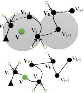
Figure 3 shows an example of insertion with the use of the aforementioned method.
Figure3. A sample of a run of the GENI algorithm
4-1-3- PRIMAL-1 algorithm
In this algorithm, with the aim of minimizing the objective function of𝐹𝐹(𝑐𝑐𝑛𝑛, 𝑏𝑏𝑛𝑛), the travelling path of vehicle is determined, in which, cn is the value added to the objective function after the selection of
the n node to pass through, and bn is the number of the covered nodes after visiting the n node.
The function F is defined as below based on Hachicha et al (2000). Based on this function, if a node, adds less cost, or covers more nodes, it has a greater priority.
2
( , )
log n
n
n n b
C F c b =
The stages of this algorithm are as follows:
1- Calculate the value of the function F for the unpassed nodes.
2- Among the unpassed nodes out of p nodes (which is obtained as 3 through trial and error), with the lowest value of the F function, select one of them randomly and set that node as the transit node, and remove all the covered nodes, from the list of the unpassed nodes.
3- Repeat stages 1 to 3, until the list of the unpassed nodes are emptied.
)
10
4-1-4- PRIMAL-2 algorithm
This algorithm is like primal-1 algorithm with the difference that the function F, equals the number of the nodes covered by each of the visited nodes (bn) and the goal is to select nodes with the highest
amount of F.
4-1-5- Nearest Neighbor (NN) algorithm
In this algorithm, first the nearest node to depot is selected as the first visited node, and then all the covered nodes, are assigned to the transit nodes. Then, among P number of nearest nodes to the last visited node (P is obtained as 3 through trial and error), one is randomly selected as the next visited node, and this process continues until all the nodes are either visited or covered (Snyder and Daskin ,2006 ).
4-2- Optimization heuristic algorithms
In local search methods, some changes are applied to an available response so it would be improved. In this research, the 3 methods below, are used to create neighborhood.
4-2-1- Node replacement inside a path (LS1)
The location of two visited nodes inside a path, are replaced.
Figure4. an example of node replacement inside a path
4-2-2-Replacement of covering and uncovering nodes (LS2)
This part, examines the possibility of replacing a covered node with its covering node (visited node). All the transit nodes of a vehicle, are selected one by one, and all the possible replacements with the nodes under cover are investigated and the best change, is reported.
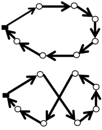
4-2-3-2-OPT algorithm (LS3) (Croes, 1958)
In this algorithm, if the number of transit nodes equals n, by selecting the two nodes of i and j among n transit nodes, path changing, is done like in figure 5.
Figure 5.A sample of 2-OPT
5- Numerical results
In this section, first the performance of the proposed heuristics are investigated in small scale, and the results are compared with accurate responses. In the second section, the performance of the proposed algorithms are examined and in the final section, the effect of the local search methods on the performance of the proposed algorithms are investigated.
5-1- The results in small scale examples
In the first stage, to compare the performance of the proposed heuristic methods, 5 sample problems in small scale and 10 sample problems in large scale, are considered. In small scale, the optimal response of the problems was obtained using the Gomez software with 3600s time limit. It should be noted that each of the heuristics for each problem, was repeated 10 times, and the mean results are given in table 1 and 2. In these tables, the first column shows the problem number and |V| shows the number of visited nodes. |W| shows the number of the nodes that should be covered. M shows the mean of the objective function of each problem, and R, shows the change percentage between the responses created in 10 repetitions based on equation 11. Also, GAP, shows the error percentage of the algorithm and is obtained from the equation below. In equation (12),
Z
maxandZ
min are the maximum and minimum values of the objective function in 10 repetitions of the algorithm.) 11 (
max min
max
Z Z
R
Z
− =
)
12
(
LS best LS
Z Z
GAP
Z
− =
In equation (11), Zls is the best response obtained from the desired heuristic algorithm and Zbest is the
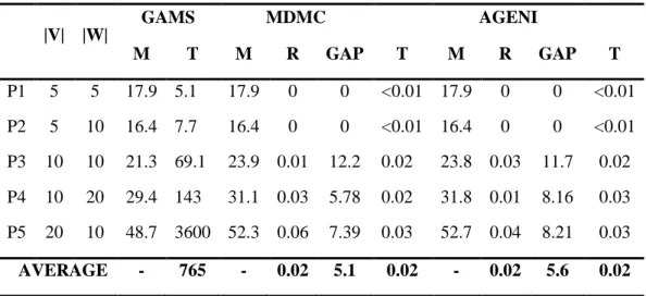
Table1. The summary of the results obtained from solving 5 problems in small scale by the accurate method and the proposed algorithms
|V| |W|
GAMS MDMC AGENI
M T M R GAP T M R GAP T
P1 5 5 17.9 5.1 17.9 0 0 <0.01 17.9 0 0 <0.01
P2 5 10 16.4 7.7 16.4 0 0 <0.01 16.4 0 0 <0.01
P3 10 10 21.3 69.1 23.9 0.01 12.2 0.02 23.8 0.03 11.7 0.02
P4 10 20 29.4 143 31.1 0.03 5.78 0.02 31.8 0.01 8.16 0.03
P5 20 10 48.7 3600 52.3 0.06 7.39 0.03 52.7 0.04 8.21 0.03
AVERAGE - 765 - 0.02 5.1 0.02 - 0.02 5.6 0.02
Table 2.The summary of the results obtained from solving 5 problems in small scales by the PRIMAL1, PRIMAL2 and NN algorithms.
|V| |W|
PRIMAL1 PRIMAL2 NN
M R GAP T M R GAP T M R GAP T
P1 5 5 17.9 0 0 <0.01 17.9 0 0 <0.01 17.9 0 0 <0.01
P2 5 10 16.4 0 0 <0.01 16.4 0 0 <0.01 16.4 0 0 <0.01
P3 10 10 25.1 0 17.8 <0.01 24.8 0 16.4 <0.01 23.8 0.01 11.7 <0.01
P4 10 20 35.8 0.01 21.8 0.02 38.6 0.03 31.3 0.02 38.1 0.08 29.6 0.02
P5 20 10 59.4 0.02 22 0.03 59.4 0.05 22 0.03 56.4 0.05 15.8 0.02
AVERAGE - 0.01 12.3 0.01 - 0.02 13.9 0.01 - 0.03 11.4 0.01
As it is clear from the results, the proposed algorithms with the mean errors of 5.1% and 5.6%, showed a better performance compared to the existing algorithms. Also, all the heuristic algorithms in 2 of the problems out of the 5 problems, resulted in the optimal response. In view of CPU time, all algorithms have good performance with average time smaller than 0.02 second.
5-2- The results in large scale examples
To compare the performance of proposed methods in large scale problems, 10 problems are considered. In tables 3 and 4, the summary of the results from running different heuristic methods are shown.
Table3. The summary of the results from running two proposed heuristic methods in large scale
|V| |W|
MDMC AGENI
M R T GAP M R T GAP
P6 20 20 59.7 0.04 0.04 0 61.1 0.05 0.06 2.35
P7 20 40 61.4 0.03 0.11 0 63.8 0.9 0.08 3.91
P8 50 50 97.1 0.09 0.27 1.89 95.3 0.16 0.31 0
P9 50 100 128.5 0.18 0.52 0 134.7 0.27 0.47 4.82
P10 100 100 161.8 0.29 1.03 1.44 159.5 0.34 0.99 0
P11 100 200 296.3 0.18 1.60 4 284.9 0.41 1.57 0
P12 150 150 341.1 0.49 2.41 1.16 337.2 0.58 2.64 0
P13 150 300 388.5 0.74 3.11 2.4 379.4 0.98 3.95 0
P14 200 200 497.4 0.91 3.54 5.69 470.6 1.02 5.16 0
P15 200 400 564.2 1.04 5.01 2.99 547.8 1.09 6.28 0
P6 20 20 59.7 0.04 5.44 0 61.1 0.05 7.19 2.35
P7 20 40 61.4 0.03 5.71 0 63.8 0.9 7.59 3.91
P8 50 50 97.1 0.09 6.24 1.89 95.3 0.16 8.33 0
P9 50 100 128.5 0.18 6.81 0 134.7 0.27 8.71 4.82
P10 100 100 161.8 0.29 7.98 1.44 159.5 0.34 9.42 0
P11 100 200 296.3 0.18 8.10 4 284.9 0.41 9.95 0
P12 150 150 341.1 0.49 9.86 1.16 337.2 0.58 10.37 0
P13 150 300 388.5 0.74 10.29 2.4 379.4 0.98 11.13 0
P14 200 200 497.4 0.91 11.47 5.69 470.6 1.02 12.32 0
P15 200 400 564.2 1.04 12.04 2.99 547.8 1.09 12.71 0
Table4.The summary of the results from running two proposed heuristic algorithms in large scale
|V| |W|
PRIMAL1 PRIMAL2 NN
M R T GAP M R T GAP M R T GAP
P
6
20 20 63.2 0.03 0.02 5.86 65.4 0.02 0.02 9.55 63.4 0.04 0.02 6.2P
7
20 40 64.1 0.05 0.04 4.4 64.1 0.05 0.05 4.4 64.1 0.06 0.05 4.4P
8
50 50 99.8 0.08 0.1 4.72 98.6 0.08 0.97 3.46 103.7 0.05 0.07 8.81P
9
50 100 138.6 0.09 0.28 7.86 141.2 0.06 0.23 9.88 142.6 0.19 0.19 11P
10
100 100 168.7 0.14 0.79 5.77 172.4 0.18 0.62 8.09 169.5 0.18 0.53 6.27 P11
100 200 314.5 0.39 0.91 10.4 310.8 0.34 0.88 9.09 325.7 0.26 0.96 14.3 P12
150 150 371.9 0.43 1.24 10.3 379.9 0.51 1.19 12.7 379.9 0.48 1.24 12.7 P13
150 300 421.5 0.77 1.35 11.1 434.4 0.64 1.42 14.5 456.1 0.53 1.96 20.2 P14
200 200 521.9 0.56 2.11 10.9 537.3 0.67 1.76 14.2 530.9 0.73 2.16 12.8P
15
200 400 628.6 0.83 2.41 14.8 671.9 0.91 2.31 22.7 690.2 1.07 2.75 26P
6
20 20 63.2 0.03 3.72 5.86 65.4 0.02 3.55 9.55 63.4 0.04 3.42 6.2P
7
20 40 64.1 0.05 4.08 4.4 64.1 0.05 4.72 4.4 64.1 0.06 4.25 4.4P
8
50 50 99.8 0.08 4.51 4.72 98.6 0.08 4.39 3.46 103.7 0.05 5.16 8.81P
9
50 100 138.6 0.09 5.42 7.86 141.2 0.06 5.2 9.88 142.6 0.19 5.72 11P
10
100 100 168.7 0.14 6.92 5.77 172.4 0.18 5.73 8.09 169.5 0.18 6.27 6.27 P11
100 200 314.5 0.39 7.22 10.4 310.8 0.34 7.99 9.09 325.7 0.26 6.94 14.3 P12
150 150 371.9 0.43 9.42 10.3 379.9 0.51 8.64 12.7 379.9 0.48 8.24 12.7 P13
150 300 421.5 0.77 10.07 11.1 434.4 0.64 9.23 14.5 456.1 0.53 9.07 20.2 P14
200 200 521.9 0.56 11.19 10.9 537.3 0.67 11.47 14.2 530.9 0.73 10.73 12.8 P15
200 400 628.6 0.83 11.98 14.8 671.9 0.91 12.35 22.7 690.2 1.07 11.17 26AVERAGE - 0.34 4.18 8.6 - 0.35 3.75 10.08 - 0.36 4.04 12.3
As is clear from table 3 and 4, the performance of the proposed heuristic algorithms, is better than the existing heuristic algorithms in large scale. The error rates of the proposed algorithms are 2 and 1.1%, respectively and on the opposite, the error rates of the existing algorithms, are 8.6, 10.8 and 12.3%.in view of solution time all algorithms have good performance with average time smaller than 6 seconds but the average solution time of proposed algorithms are about 6 seconds that is slightly larger than that from existing heuristic algorithms in the literature with average time about 4 second.
5-3- Investigation of the effect of local searches on the proposed algorithms’
performance
In order to investigate the effect of the combination of the local search methods on the algorithms of AGENI and MDMC, they are combined with each of the three local search methods, and implemented on the sample problems. Each of these local search methods is repeated until no further optimization resulted in the response.
In table 5, the results from the combination of the MDMC heuristic algorithm with local search methods in small scales, are shown. In this table, LS1, is the replacement method of the nodes inside a path, LS2 is the replacement of covering and uncovering nodes, and LS3, is the 2-OPT method. It's noteworthy to say that the information related to the problems, are given in tables 1 and 2.
Table5.The results from combining the MDMC method with the local search method in small scales
GAMS MDMC+LS1 MDMC+LS2 MDMC+LS3
M T M R T GAP M R T GAP M R T GAP
P1 17.9 5.1 17.9 0 0.01 0 17.9 0 0.01 0 17.9 0 0.01 0
P2 16.4 7.7 16.4 0 0.19 0 16.4 0 0.29 0 16.4 0 0.29 0
P3 21.3 69.1 22.1 0.01 0.73 3.76 22.1 0.01 0.84 3.76 21.9 0.01 0.9 2.82
P4 29.4 142.5 31.1 0.03 1.4 5.78 31.1 0.03 1.34 5.78 31.1 0.03 1.49 5.78
P5 48.7 3600 50.7 0.06 2.2 4.11 49.8 0.06 2.51 2.26 51.1 0.06 2.31 4.93
AVERAGE 764.9 - 0.02 0.906 2.7 - 0.02 0.998 2/4 - 0.02 1 2.7
As shown in table 5, the combination of the MDMC method with local search methods, causes a 2.5 per cent error rate reduction from 5% to 2.5%. The highest error has occurred at about 5.87% in the p4 problem. Among the local search methods, the replacement of the covering and uncovering nodes has had the best performance with the mean error rate of 2.4% in problems in small scales. The results from the combination of the AGENI algorithm and local searches are shown in table 6.
Table6.The results from combing the AGENI method with the local search method in small scales.
GAMS AGENI+LS1 AGENI+LS2 AGENI+LS3
M T M R T GAP M R T GAP M R T GAP
P1 17.9 5.1 17.9 0 0.01 0 17/9 0 0.01 0 17.9 0 0.01 0
P2 16.4 7.7 16.4 0 0.37 0 16/4 0 0.29 0 16.4 0 0.29 0
P3 21.3 69.1 22.1 0.03 0.84 3.76 21.1 0.03 0.86 0.94 21.9 0/03 0.9 2.82
P4 29.4 142.5 31.1 0.01 1.28 5.78 31.1 0.01 1.49 5.78 31.1 0/01 1.49 5.78 P5 48.7 3600 50.2 0.04 2.48 3.08 51.3 0.04 2.68 5.34 50.2 0/04 2.51 3.08
AVERAGE 764.9 - 0.02 0.996 2.5 - 0.02 1.066 2.4 - 0.02 1.04 2.3
As shown in table 6, the combination of the AGENI method with the 2-OPT local search method, has had the best performance in small scale problems and has offered 2.3% error. In this part, the combination with the covering and uncovering nodes replacement method is in the second place with little distance with the combination with 2-opt method.
At the end, for a more accurate examination of combined algorithms, these algorithms are implemented on 10 problems produced in large scales. The results are given in table 7.
Table7. The results from combined algorithms on 10 problems with large scales
METHODS 6P 7P 8P 9P 10P 11P 12P 13P 14P 15P Average
MDMC+LS1
M 55.7 60.2 89.4 100.7 155.3 273.4 307.9 334.9 405.2 491.9
R 0.03 0.09 0.08 0.16 0.2 0.39 0.24 0.31 0.42 0.59 0.251
T 2.4 3.9 5.2 7.1 10.4 9.6 13.4 15.2 16.8 17.1 10.11
GAP 6.5 3.26 2.64 5.56 3.19 3.44 2.02 5.61 2.12 2.08 3.642
MDMC+LS2
M 55.7 59.8 90.1 95.4 158.3 264.3 305.1 320.5 412.9 497.4
R 0.03 0.02 0.09 0.19 0.21 0.27 0.31 0.39 0.4 0.47 0.238
T 3.1 5.2 6.8 9.4 12.3 15.2 17.1 18.5 20.7 24.9 13.32
GAP 6.5 2.57 3.44 0 5.18 0 1.09 1.07 4.06 3.22 2.713
MDMC+LS3
M 52.3 60.9 89.9 100.7 156.4 270.2 301.8 320.4 407.5 496.3
R 0/02 0.07 0.09 0/16 0.27 0.34 0.31 0.44 0.49 0.59 0.278
T 2/9 4.7 5.9 8/6 11.1 14.3 16.5 17.9 19.9 22.1 12.39
GAP 0 4.46 3.21 5.56 3.92 2.23 0 1.04 2.7 2.99 2.611
AGENI+LS1
M 53.1 60.2 90.1 104.7 155.6 273.4 305.1 317.1 412.9 481.9
R 0.04 0.06 0.11 0.25 0.19 0.29 0.37 0.49 0.61 0.52 0.293
T 2.9 3.5 6.4 7.2 9/4 12.3 14.6 17.2 18.1 19.4 11.1
GAP 1.53 3.26 3.44 9.75 3.39 3.44 1.09 0 4.06 0 2.996
AGENI+LS2
M 55.7 58.3 88.3 99.3 151.7 264.3 305.1 319.5 396.8 483.1
R 0.03 0.07 0.17 0.18 0.29 0.39 0.46 0.39 0.47 0.55 0.3
T 2.8 4.1 7.5 9.6 12.8 15.9 18.3 20.9 22.4 25.6 13.99
GAP 6.5 0 1.38 4.09 0.8 0 1.09 0.76 0 0.25 1.487
AGENI+LS3
M 55.7 60.9 87.1 100.7 150.5 269.1 305.1 317.1 407.5 491.9
R 0.04 0.09 0.26 0.24 0.31 0.44 0.31 0.35 0.47 0.51 0.302
T 2.6 3.9 7.1 8.5 11.3 15.2 16.9 19.3 21/5 24.9 13.12
GAP 6.5 4.46 0 5.56 0 1.82 1.09 0 2/7 2.08 2.421
As shown in table 7, among the 10 problems, the combined methods based on MDMC in 4 problems, could result the best possible response and the combined methods with AGENI, could, in 6 problems, offer the best possible responses. Also, the produced heuristic algorithms which used LS2, have gained the highest share in finding the best possible response (4 problems out of 10). In figure 6, the mean error, changesmean and meantime to resolve are shown for each of the 6 combined algorithms.
Figure6. The error, changes and time to resolve of 6 combined algorithms on 10 problems with large scale
As it is clear from figure 6, the LS2 local search method, has a higher time to resolve compared to LS1 and LS3, when combined with MDMC or AGENI. Also, the time to resolve of each of the combined methods which used the AGENI response production algorithm, is longer than the combined methods which used MDMC.But the lowest possible error has occurred in the combined algorithms of AGENI with LS2. On the one hand, this combined algorithm has the highest time to resolve. Concerning the changes of response, also, almost all the methods, showed similar changes.
6. Conclusion
In this research, two new heuristic algorithms were introduced for CTP. In order to investigate the performance of the proposed heuristics in small scale, 5 sample problems were solved with exact method, and the results of them, were compared with the results of the proposed algorithms. In the following, 10 sample large scale problems were solved and the proposed heuristic algorithms were compared with the existing heuristics. In these scales, the mean error rate of the proposed algorithms were 2% and 1.1% respectively, while the error of the existing methods in the literature was about 10%. At the end, in order to investigate the effect of the local search methods on the quality of the response, two of the proposed algorithms were combined with three local search methods and were compared in large and small scales. In small scales, the error for the proposed algorithms deceased from about 5% to 2.5%. In large scales, the mean error rate, had a proper decrease.
References
Arkin E. M. and Hassin R.,(1994)."Approximation algorithms for the geometric covering salesman problem," Discrete Applied Mathematics, vol. 55, pp. 197-218.
Croes G.,(1958). "A method for solving traveling-salesman problems," Operations Research, vol. 6, pp. 791-812.
Current J. R. and Schilling D. A.,(1989). "The covering salesman problem," Transportation science, vol. 23, pp. 208-213.
Current J. R. and Schilling D. A.,(1994). "The median tour and maximal covering tour problems: Formulations and heuristics," European Journal of Operational Research, vol. 73, pp. 114-126.
3. 64 2 2. 71 3 2. 61 1 2. 99 6 1. 48
7 2.421
10 .1 1 13 .3 2 12 .3 9 11 .1 13 .9 9 13 .1 2 0. 25 1 0. 23 8 0. 27 8 0. 29 3 0. 3 0. 30 2
M D M C + L S 1 M D M C + L S 2 M D M C + L S 3 A G E N I + L S 1 A G E N I + L S 2 A G E N I + L S 3 GAP T R
Daskin M.,(1995). "Network and discrete location analysis," ed: John Wiley and Sons, New York. Fischetti M. and Toth P.,(1988). "AN ADDITIVE APPROACH FOR THE OPTIMAL SOLUTION OF THE PRIZE-COLLECTING TRAVELLING SALESMAN PROBLEM. VEHICLE ROUTING: METHODS AND STUDIES. STUDIES IN MANAGEMENT SCIENCE AND SYSTEMS-VOLUME 16," Publication of: Dalctraf.
Gendreau M., Hertz A., and Laporte G.,(1992). "New insertion and postoptimization procedures for the traveling salesman problem," Operations Research, vol. 40, pp. 1086-1094.
Golden B., Naji-Azimi Z., Raghavan S., Salari M., and Toth P.,(2012). "The generalized covering salesman problem," INFORMS Journal on Computing, vol. 24, pp. 534-553.
Hachicha M., John Hodgson M., Laporte G., and Semet F.,(2000). "Heuristics for the multi-vehicle covering tour problem," Computers & Operations Research, vol. 27, pp. 29-42.
Hodgson M. J., Laporte G., and Semet F., (1998). "A Covering Tour Model for Planning Mobile Health Care Facilities in SuhumDistrict, Ghama," Journal of Regional Science, vol. 38, pp. 621-638. Labbé M., Laporte G., Martín I. R., and González J. J. S.,(2004). "The ring star problem: Polyhedral analysis and exact algorithm," Networks, vol. 43, pp. 177-189.
Jozefowiez N., Semet F., and Talbi E.-G.,(2007). "The bi-objective covering tour problem," Computers & operations research, vol. 34, pp. 1929-1942.
Jozefowiez, N. (2014). A branch‐and‐price algorithm for the multivehicle covering tour problem. Networks, 64(3), 160-168.
Laporte G. and Martello S.,(1990). "The selective travelling salesman problem," Discrete applied mathematics, vol. 26, pp. 193-207.
Lin S. and Kernighan B. W.,(1973). "An effective heuristic algorithm for the traveling-salesman problem," Operations research, vol. 21, pp. 498-516.
Moreno Pérez J. A., Marcos Moreno-Vega J., and Rodrı́guez Martı́n I.,(2003). "Variable neighborhood tabu search and its application to the median cycle problem," European Journal of Operational Research, vol. 151, pp. 365-378.
Naji-Azimi Z. and Salari M.,(2014). "The time constrained maximal covering salesman problem," Applied Mathematical Modelling, vol. 38, pp. 3945-3957.
Salari M., Reihaneh M., and Sabbagh M. S.,(2015). "Combining ant colony optimization algorithm and dynamic programming technique for solving the covering salesman problem," Computers & Industrial Engineering.
Nolz P. C., Doerner K. F., Gutjahr W. J., and Hartl R. F.,(2010). "A bi-objective metaheuristic for disaster relief operation planning," in Advances in multi-objective nature inspired computing, ed: Springer, pp. 167-187.
Salari M. and Naji-Azimi Z.,(2012). "An integer programming-based local search for the covering salesman problem," Computers & Operations Research, vol. 39, pp. 2594-2602.
Schilling D. A., Jayaraman V., and Barkhi R., (1993). "A REVIEW OF COVERING PROBLEMS IN FACILITY LOCATION," Computers & Operations Research.
Snyder L. V. and Daskin M. S.,(2006). "A random-key genetic algorithm for the generalized traveling salesman problem," European Journal of Operational Research, vol. 174, pp. 38-53.
Tricoire F., Graf A., and Gutjahr W. J.,(2012). "The bi-objective stochastic covering tour problem," Computers & operations research, vol. 39, pp. 1582-15922.