172
Multi-objective optimization of population partitioning problem
under interval uncertainty
Foroogh ghollasi mood
1, Hasan Hosseini-Nasab
1*, Mohammad Bagher Fakhrzad
1,
javad Tayyebi
2Industrial Engineering Department, Yazd University, Yazd, Iran
Industrial Engineering Department, Birjand University of Technology, Birjand, Iran [email protected], [email protected], [email protected], [email protected]
Abstract
This paper addresses a bi-objective mixed integer optimization model under uncertainty for population partitioning problem. The objective functions are to minimize the number of communications between partitions and to balance their population. The main constraints are defined for creating contiguous and compact partitions as well as assigning uniquely each basic unit to one partition. To deal with the uncertainty of parameters, a robust programming method is proposed that causes the uncertainty parameters lie between the interval of best-case (the deterministic mode) and worst-best-case (the highest uncertainty level for all parameters). As the suggested method is NP-Hard, three meta-heuristic algorithms NSGAII, PESA, and SPEA are developed and, to evaluate the efficiency of the algorithms, 10 small-size examples, 10 medium-size examples and, 10 large-size examples are generated and solved. According to computational results, the SPEA has the best performance. The method is examined for a real-world application, as a case study in Iran.
Keywords: Partitioning, interval uncertainty, multi-objective optimization, robust programming.
1-Introduction
Population partitioning problem is generally defined as grouping basic units to partitions (Garfinkel & Nemhauser, 1970). Optimal partitions in a territory should have features, such as balance (population size, distance from each other and unemployment rate), contiguousness, compactness, and the absence of holes (Baqir, 2002). To solve partitioning problems in real-world applications, it is necessary to show connections between territories as a network structure (Liberatore & Camacho-Collados, 2016). This structure is an undirected graph 𝐺 = (𝑉, 𝐸) with vertex set 𝑉 (cities or basic units) and connection set 𝐸. Any population partitioning problem can be regarded as a graph partitioning problem (Tran, Dinh, & Gascon, 2017).
Many studies have been done on partitioning application in different fields. One of the earliest studies belongs to Ghiggi et al. (Ghiggi, Puliafito, & Zoppoli, 1975). There, each partition is composed of a certain number of inseparable communities with centralized population. Minciardi et al. studied decomposition of a geographic territory into an indefinite number of non-overlapping partitions.
*Corresponding author
ISSN: 1735-8272, Copyright c 2020 JISE. All rights reserved
Journal of Industrial and Systems Engineering Vol. 12, No. 4, pp. 172 - 197
173
They introduced two heuristic algorithms to achieve compact primary areas for reducing calculations process in partitions (Minciardi, Puliafito, & Zoppoli, 1981). Pezzella et al. addressed partitioning problem with optimal allocation of services (Pezzella, Bonanno, & Nicoletti, 1981). Lin and Kao introduced a mixed integer optimization model to partition municipal solid waste collection sites (H.-Y. Lin & Kao, 2008). Chen and Yum presented a new public security criterion to define security function level (Chen & Yum, 2010). Benzarti et al. addressed partitioning problem to deal with home health care services. Their contribution was formulating home health care partitioning problem as a mixed integer programming model with some criteria, such as basic units separation, compactness, workload balance between human resources, and consistency (Benzarti, Sahin, & Dallery, 2013). De Assis et al. investigated balanced multi-criteria partitioning problem for electricity meter reading based on compactness and homogeneity criteria of partitions (De Assis, Franca, & Usberti, 2014). Butsch et al. proposed a heuristic algorithm for arc routing districting problem (Butsch, Kalcsics, & Laporte, 2014). Camacho-Collados et al. studied multi-criteria police districting problem for the first time. They considered some area criteria, such as risk, compactness, and mutual support (Camacho-Collados, Liberatore, & Angulo, 2015). García‐Ayala et al. solved road network partitioning problem with a certain number of partitions by an integer mathematical model..
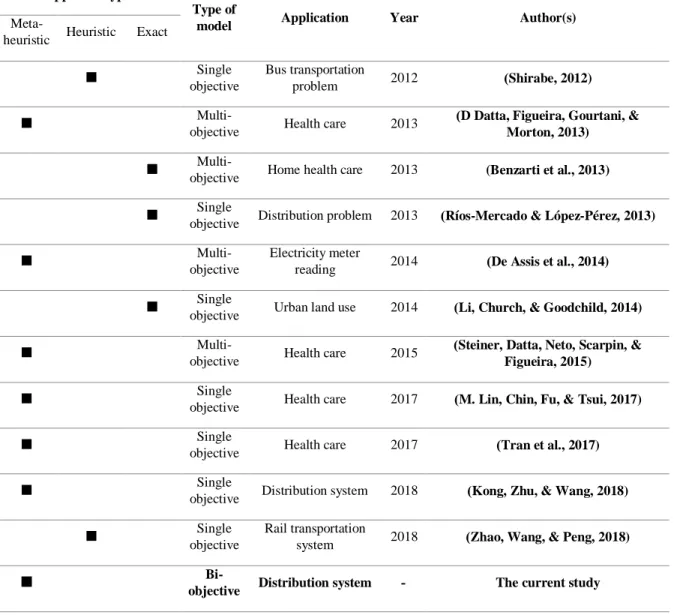
Table 1. Studies in the field of graph partitioning with emphasize on solution methods Author(s) Year Application Type of model Approach type Exact Heuristic Meta-heuristic )Shirabe, 2012) 2012 Bus transportation problem Single objective
)D Datta, Figueira, Gourtani, & Morton, 2013) 2013 Health care Multi-objective
(Benzarti et al., 2013) 2013
Home health care
Multi-objective
)Ríos-Mercado & López-Pérez, 2013) 2013
Distribution problem Single
objective
)De Assis et al., 2014) 2014 Electricity meter reading Multi-objective
)Li, Church, & Goodchild, 2014) 2014
Urban land use Single
objective
)Steiner, Datta, Neto, Scarpin, & Figueira, 2015) 2015 Health care Multi-objective
)M. Lin, Chin, Fu, & Tsui, 2017) 2017
Health care Single
objective
)Tran et al., 2017) 2017
Health care Single
objective
)Kong, Zhu, & Wang, 2018) 2018
Distribution system Single
objective
)Zhao, Wang, & Peng, 2018) 2018 Rail transportation system Single objective
The current study -
Distribution system
Bi-objective
174
This problem was taken into consideration by many organizations including post offices, municipalities for urban and winter services, road maintenance, and urban waste disposal sections (García‐Ayala, González‐Velarde, Ríos‐Mercado, & Fernández, 2016)
To solve partitioning problems, many methods have been developed mainly based on meta-heuristic algorithms. In addition to the well-known genetic algorithm, some other meta-heuristic algorithms have been used to solve partitioning problem, such as simulated annealing (Brooks & Morgan, 1995), tabu search (Bozkaya, Erkut, & Laporte, 2003), hybrid simulated annealing and tabu-search (Baños, Gil, Paechter, & Ortega, 2007), particle swarm (Wang, Wu, & Mao, 2007), and differential evolution (Dilip Datta & Figueira, 2011).
In this paper, population partitioning problem is proposed as a bi-objective problem with the aim of minimizing connections between basic units outside a partition and balancing the population in partitions under uncertainty conditions. To deal with uncertainty of parameters, the optimization method provided by Sim and Bertsimas (Bertsimas & Sim, 2004) is applied.
The remainder of this paper is organized as follows. The problem definition is given in section 2. Solution methods and the related explanations are presented in section 3. In section 4, the proposed algorithms are compared with the mathematical model. The efficiency of algorithms is assessed in section 5. The case study is investigated in section 6. Finally, conclusions are presented in section 7.
2-Problem statement
Assume 𝐺 = (𝑉, 𝐸) is an undirected graph with vertex set 𝑉 (basic units) and edge set 𝐸. The vertex set 𝑉 contains 𝑁 vertices 𝑣1, 𝑣2, … , 𝑣𝑁. Each vertex 𝑣𝑖 is represented by a pair (𝑥𝑖, 𝑦𝑖) of vertical and
horizontal coordinates. Any edge of G with two endpoints 𝑣𝑖 and 𝑣𝑗is denoted by (𝑣𝑖, 𝑣𝑗). Each vertex 𝑣𝑖
has a weight 𝑤𝑖 ≥ 0, and it can be considered as 𝑤𝑖𝑗 = 𝑤𝑖+ 𝑤𝑗 for each pair of vertices 𝑣𝑖 and 𝑣𝑗. These
weights represent some characteristics, such as population and demand for each vertex. Since the adjacency matrix corresponding to G is symmetric, it follows that𝑤𝑖𝑗 = 𝑤𝑗𝑖. We can also consider 𝑊 = (𝑤𝑖𝑗) as an adjacency matrix. If 𝑤𝑖𝑗 > 0, then there is an edge between vertices 𝑣𝑖 and 𝑣𝑗. If 𝑤𝑖𝑗 = 0,
there is not any edge joining vertices 𝑣𝑖 and 𝑣𝑗. In addition, another parameter 𝑝𝑖𝑗 represents the
population difference between vertices 𝑣𝑖 and 𝑣𝑗. In fact, this serves as a parameter to balance the
population in partitions.
Suppose that the goal is to divide vertices into the set of partitions P. We denote by |𝑃| the number of elements belonging to P. So 𝑃 = {1,2, … , |𝑃|}. Let the values 𝐶𝑚𝑖𝑛 and 𝐶𝑚𝑎𝑥 respectively represent the
minimum and maximum number of vertices that can be placed in a partition. It is clear that 𝑃 ∈ {2, … , 𝑁 − 1}, 𝐶𝑚𝑖𝑛, 𝐶𝑚𝑎𝑥∈ {1, … , 𝑁} and 𝐶𝑚𝑖𝑛 ≤ 𝐶𝑚𝑎𝑥. Let 𝑋𝑖𝑝 be a binary variable that equals to one
if vertex 𝑣𝑖 is assigned to partition 𝑝 ∈ {1, … , |𝑃|}, and otherwise 𝑋𝑖𝑝= 0. Another binary variable 𝑌𝑖𝑗
equals to one if vertices 𝑣𝑖 and 𝑣𝑗 are not assigned to the same partition, and otherwise 𝑌𝑖𝑗= 0. The
objective function of partitioning problem is to minimize the total weight of edges that are considered as connections between two partitions. Since the adjacency matrix corresponding to G is symmetric, the objective function can be defined as min1
2∑ 𝑌𝑖,𝑗 𝑖𝑗𝑤𝑖𝑗 or min ∑𝑖≤𝑗𝑌𝑖𝑗𝑤𝑖𝑗. According to these definitions,
the mathematical model of the problem is expressed in equations (1) to (7). Input parameters
𝑤𝑖𝑗 Number of required transfers between vertices 𝑣𝑖 and 𝑣𝑗 (the transferred population between
vertices).
𝑝𝑖𝑗 Difference between populations of vertices 𝑣𝑖 and 𝑣𝑗. M A positive and large enough scalar
175
2-1-Mathematical formulation
Model 1
(1.a) 𝑀𝑖𝑛 ∑ ∑ 𝑌𝑖𝑗𝑤𝑖𝑗
𝑗=𝑖+1 𝑖∈𝑉
,
(1.b) 𝑀𝑖𝑛 ∑ ∑ 𝑌𝑖𝑗𝑝𝑖𝑗
𝑗=𝑖+1 𝑖∈𝑉
, 𝑠. 𝑡.
(2) ∀𝑖 ∈ 𝑉,
∑ 𝑋𝑖𝑝 𝑝∈𝑃
= 1,
(3) ∀𝑝 ∈ 𝑃,
𝐶𝑚𝑖𝑛 ≤ ∑ 𝑋𝑖𝑝 𝑖∈𝑉
≤ 𝐶𝑚𝑎𝑥,
(4) ∀𝑖, 𝑗 ∈ 𝑉, 𝑝 ∈ 𝑃,
−𝑌𝑖𝑗− 𝑋𝑖𝑝+ 𝑋𝑗𝑝 ≤ 0,
(5) ∀𝑖, 𝑗 ∈ 𝑉, 𝑝 ∈ 𝑃,
−𝑌𝑖𝑗+ 𝑋𝑖𝑝− 𝑋𝑗𝑝 ≤ 0,
(6) ∀𝑖, 𝑗 ∈ 𝑉, 𝑝 ∈ 𝑃,
∑ 𝑋𝑟𝑝 𝑟∈𝐻𝑖𝑗
≥ 𝑆𝑃𝑖𝑗− 𝑀 (2 − (𝑋𝑗𝑝+ 𝑋𝑖𝑝)),
(7) ∀𝑖, 𝑗 ∈ 𝑉, 𝑝 ∈ 𝑃,
𝑋𝑖𝑝∈ {0,1}, 𝑌𝑖𝑗∈ {0,1},
The first objective function is to minimize the total weight of connections between partitions. The second objective function balances the population in partitions as much as possible. Constraint (2) ensures that each vertex is assigned to only one partition. Constraint (3) guarantees that the number of vertices in each partition is between the upper and lower bounds. Constraints (4) and (5) state that if vertices 𝑣𝑖 and 𝑣𝑗are not in the same partition, then 𝑌𝑖𝑗 = 1, otherwise 𝑌𝑖𝑗= 0. Constraint (6) is the first provided
mathematical formulation maintaining continuity, compactness, and the absence of holes. 𝑆𝑃𝑖𝑗 is the set
of vertices on the shortest path between vertices 𝑣𝑖 and 𝑣𝑗, and |𝑆𝑃𝑖𝑗| is the number of its vertices.
Constraint (7) specifies the range of variables.
One of the most prominent characteristics of this model is that it considers the fundamental constraints of the partitioning problem (contiguity and compactness partitions). No integrated, specific mathematical model has been presented yet since the constraints are difficult to design (Kalcsics. J, 2015). The constraint (6) states that the shortest path between each two basic units belonging to a single partition must be located inside that partition. Thus, all of the points on the shortest path between the two basic units are inside that partition as well. This constraint not only assures contiguity and avoidance of unusual partition allocations but also causes partitions with the feature of compactness to be generated. In the final partitioning, therefore, the generated partitions are expected to be convex as far as possible, and no unusual allocation is expected to exist. However, points on shortest path between each two basic units can be specified using some common algorithms like Dijkstra’s algorithm. In this algorithm, the shortest-path tree will be formed if the algorithm is run for all the points in the area under investigation. It should be noted that there is not one communication path between each of the two points (corners) in the graph network used in this research, unlike in communication networks between populated areas. The relations between points will be in the form of a graph network. This can be observed more clearly in the case study of the research. However, a question that may be raised is how path selection will work if there is more than one shortest path between two different vertices. To respond to this question, one can consider the structure of the algorithm used for finding the shortest path (Dijkstra’s algorithm in this research). As stated, the shortest-path tree will be generated if the algorithm is run for all the vertices in the area. Therefore, two shortest paths are never identified between two specific vertices, since the eventual structure would then involve a cycle, and would no longer be a tree, and this would be a contradiction in
176
the algorithm structure. It can, therefore, be assured that the points on the shortest path between two vertices are identified by the algorithm that is used.
A point to must be clarified is the difference between the parameters 𝑝𝑖𝑗 and 𝑤𝑖𝑗 and their
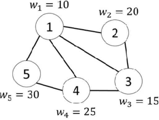
computational structure in the mathematical model. Let us illustrate it by one example. Assume that the network contains 5 vertices with populations of 10, 20, 15, 25, and 30 shown in figure 1.
Fig 1. A graphic structure of problem
Therefore, one can say that 𝑝12= 𝑝21= 10, 𝑝23= 𝑝32= 5, 𝑝34= 𝑝43= 10, 𝑝45= 𝑝54= 5, 𝑝14= 𝑝41= 15, 𝑝13= 𝑝31= 5, and 𝑝15= 𝑝51= 20. Moreover, parameter 𝑤𝑖𝑗 is randomly specified
according to the following numbers. 𝑤12= 𝑤21= 20
𝑤23= 𝑤32 = 15 𝑤34= 𝑤43= 15 𝑤45= 𝑤54= 20 𝑤14= 𝑤41 = 10 𝑤13= 𝑤31= 15 𝑤15= 𝑤51= 10
As stated before, 𝑝𝑖𝑗 can be calculated through the population of vertices; however, 𝑤𝑖𝑗 is a parameter
that is independently entered by the decision maker. For example, it can indicate the amount of demands that should be moved between adjacent vertices. This work has several practical applications in health care system management and supply chain management. In fact, 𝑝𝑖𝑗 is used to create population balance
in partitions while 𝑤𝑖𝑗 aims to minimize the number of trips between partitions. For example, in
healthcare system, it is assumed that some people from a certain basic unit have to go to adjacent basic units to receive healthcare services. If vertices 1, 2, and 3 are supposed to be in a partition and vertices 4 and 5 in another partition, value of the first and the second objective functions will be 45 and 35 based on objective functions (a.1) and (b.1), respectively. If the partition structure is changed and vertices 1 and 2 are located in one partition and vertices 3, 4, and 5 in the other partition, then the first and the second objective values will be 35 and 50, respectively. As can be seen, different partition structures are non-dominated; therefore, one cannot choose an ideal solution definitely. In fact, this example demonstrates that the provided objective functions are generally contradictory and can be considered as different objective functions.
2-2-
Robust mathematical formulation
In this paper, the investigated uncertainty is related to matrices 𝑊 = (𝑤𝑖𝑗)𝑁×𝑁and 𝑃 = (𝑝𝑖𝑗)𝑁×𝑁. Each
component 𝑤𝑖𝑗 is modeled randomly as an indeterminate symmetric distribution parameter bounded to 𝑤̂𝑖𝑗 which varies in the interval [𝑤𝑖𝑗− 𝑤̂𝑖𝑗, 𝑤𝑖𝑗+ 𝑤̂𝑖𝑗]. It is noteworthy that parameter 𝑤̂𝑖𝑗 is the constant
177
part and 𝑤𝑖𝑗 is the variable part. Therefore, one can state 𝑤̂𝑖𝑗 = 𝑤̂𝑗𝑖 for 𝑖, 𝑗 = 1, … , 𝑁. Similarly, the same
definitions can be proposed for parameter 𝑝𝑖𝑗. Based on Sim and Bertsimas robust programming
(Bertsimas, 2004), the uncertainty conditions for parameter 𝑤𝑖𝑗 is first described, and then it is considered
similarly for parameter 𝑝𝑖𝑗.
Robust optimization is proposed to investigate uncertainty of weight matrix W by means of 𝑤̃𝑖𝑗 = [𝑤𝑖𝑗− 𝑤̂𝑖𝑗, 𝑤𝑖𝑗+ 𝑤̂𝑖𝑗], where 𝑤𝑖𝑗 is the nominal value of edge (𝑣𝑖, 𝑣𝑗). J is the set of indices related to W
with uncertain changes i.e. 𝐽 = {(𝑖, 𝑗): 𝑤̂𝑖𝑗 > 0, 𝑖 = 1, . . , 𝑁, 𝑗 = 𝑖 + 1, … , 𝑁}. It is supposed that 𝛤 is a
parameter that is not necessarily integer and gets value in the interval [0, |𝐽|]. This parameter was introduced by Bertsimas and Sim (Bertsimas & Sim, 2003) to adjust robustness of the proposed method against conservative level of introduced solution. The number of coefficients 𝑤𝑖𝑗 and 𝑤𝑖𝑡𝑗𝑡are allowed to be changed at most ⌊𝛤⌋ and (𝛤 − ⌊𝛤⌋), respectively. The subscript of i and j is t which is explained in the following. In Bertsimas robust programming, the number of uncertain parameters varies proportional to value of the robustness parameter, so there should be a counter in the set of main counters that counts the uncertain parameters. For instance, if we have 10 basic units, there will be 100 number of w. Assume that based on value of the robustness parameter, only 10 of them are uncertain, and the rest remain at the upper bound. Hence, a counter is required to count those 10. The index t does the same as explained. Therefore, robust partitioning problem can be formulated as follows.
Model 2
min (𝑋𝑖𝑝,𝑌𝑖𝑗)
(∑ ∑ 𝑌𝑖𝑗𝑤𝑖𝑗 𝑗=𝑖+1 𝑖∈𝑉
+ max
{𝑆:𝑆⊆𝐽,|𝑆|≤𝛤 (𝑖𝑡𝑗𝑡)∈𝐽/𝑆}
( ∑ 𝑌𝑖𝑗𝑤̂𝑖𝑗 (𝑖,𝑗)∈𝑆
+ (𝛤 − ⌊𝛤⌋) 𝑤̂𝑖𝑡𝑗𝑡𝑌𝑖𝑡𝑗𝑡)), (8)
𝑠. 𝑡.
𝐶𝑜𝑛𝑠𝑡𝑟𝑎𝑖𝑛𝑡𝑠 (2) − (6).
Notice that there are different conditions based on the selected value 𝛤.
If 𝛤 = 0, no change is allowed and the problem is decreased to a nominal one like to Model 1. If 𝛤 is selected as an integer number, the value of the objective function (8) will equal to
max
{𝑆|𝑆⊆𝐽,|𝑆|≤𝛤 }∑(𝑖,𝑗)∈𝑆𝑌𝑖𝑗𝑤̂𝑖𝑗 at most.
If 𝛤 = |𝐽|, the problem can be solved by the Swister method (Fan, Zheng, & Pardalos, 2012). As stated in (Fan et al., 2012), the objective function (8) can be equivalently formulated as a mixed binary linear programming.
The method used in the proof of the following theorem was proposed by (Bertsimas & Sim, 2004) for the first time.
Theorem: Model 2 is equivalent to the following mixed binary linear programming formulation.
Model 3
(9) 𝑀𝑖𝑛 ∑ ∑ 𝑌𝑖𝑗𝑤𝑖𝑗
𝑁
𝑗=𝑖+1 𝑖∈𝑉
+ 𝛤 𝑈0+ ∑ 𝑈𝑖𝑗 (𝑖,𝑗)∈𝐽
, 𝑠. 𝑡.
178
(10) ∀𝑖 ∈ 𝑉,
∑ 𝑋𝑖𝑝 𝑝∈𝑃
= 1,
(11) ∀𝑝 ∈ 𝑃,
𝐶𝑚𝑖𝑛 ≤ ∑ 𝑋𝑖𝑝 𝑖∈𝑉
≤ 𝐶𝑚𝑖𝑛,
(12) ∀𝑖, 𝑗 ∈ 𝑉, 𝑝 ∈ 𝑃,
−𝑌𝑖𝑗− 𝑋𝑖𝑝+ 𝑋𝑗𝑝 ≤ 0,
(13) ∀𝑖, 𝑗 ∈ 𝑉, 𝑝 ∈ 𝑃,
−𝑌𝑖𝑗+ 𝑋𝑖𝑝− 𝑋𝑗𝑝 ≤ 0,
(14) ∀(𝑖, 𝑗) ∈ 𝐽,
𝑈0+ 𝑈𝑖𝑗− 𝑌𝑖𝑗𝑤̂𝑖𝑗≥ 0,
(15) ∀𝑖, 𝑗 ∈ 𝑉, 𝑝 ∈ 𝑃,
∑ 𝑋𝑟𝑝 𝑟∈𝐻𝑖𝑗
≥ 𝑆𝑃𝑖𝑗− 𝑀 (2 − (𝑋𝑗𝑝+ 𝑋𝑖𝑝)),
(16) ∀(𝑖, 𝑗) ∈ 𝐽,
𝑈𝑖𝑗≥ 0,
(17) 𝑈0≥ 0,
(18) ∀𝑖, 𝑗 ∈ 𝑉, 𝑝 ∈ 𝑃.
𝑋𝑖𝑝∈ {0,1}, 𝑌𝑖𝑗∈ {0,1} ,
Proof: For any given value of (𝑌𝑖𝑗)𝑖=1,…,𝑁 ,𝑗=𝑖+1,…,𝑁in Model 2, max {𝑆:𝑆⊆𝐽,|𝑆|≤𝛤
(𝑖𝑡𝑗𝑡)∈𝐽/𝑆}
(∑(𝑖,𝑗)∈𝑆𝑌𝑖𝑗𝑤̂𝑖𝑗+ (𝛤 − ⌊𝛤⌋) 𝑤̂𝑖𝑡𝑗𝑡𝑌𝑖𝑡𝑗𝑡) can be linearized by introducing 𝑧𝑖𝑗 for all (𝑖, 𝑗) ∈ 𝐽 subject to constraints
∑(𝑖,𝑗)∈𝐽𝑧𝑖𝑗≤ 𝛤and 0 ≤ 𝑧𝑖𝑗≤ 1, as shown in Model 4.
Model 4
𝑚𝑖𝑛 ∑(𝑖,𝑗)∈𝑆𝑌𝑖𝑗𝑤̂𝑖𝑗𝑧𝑖𝑗, (19)
𝑠. 𝑡.
∑(𝑖,𝑗)∈𝐽𝑧𝑖𝑗≤ 𝛤, (20)
0 ≤ 𝑧𝑖𝑗 ≤ 1, ∀(𝑖, 𝑗) ∈ 𝐽. (21)
This formulation is a fractional knapsack problem with bound constraints. The optimal solution of this formulation should have ⌊𝛤⌋ variables 𝑧𝑖𝑗 = 1 and one 𝑧𝑖𝑗 = 𝛤 − ⌊𝛤⌋ that is equivalent to the optimal
solution in maximization part of Model 2. Model 4 is linear for the given values of (𝑌𝑖𝑗)𝑖=1,…,𝑁 ,𝑗=𝑖+1,…,𝑁.
Its duality can be formulated as follows:
Model 5
(22) 𝑀𝑖𝑛 𝛤 𝑈0+ ∑ 𝑈𝑖𝑗
(𝑖,𝑗)∈𝐽 , 𝑠. 𝑡.
(23) ∀(𝑖, 𝑗) ∈ 𝐽,
𝑈0+ 𝑈𝑖𝑗− 𝑌𝑖𝑗𝑤̂𝑖𝑗≥ 0,
(24) ∀(𝑖, 𝑗) ∈ 𝐽.
𝑈𝑖𝑗≥ 0,
(25) 𝑈0≥ 0,
Model 3 can be obtained by combining models 5 and 2. This completes the proof.
On account of the fact that the proposed model has a linear structure, it can be solved as a mixed binary programming model by CPLEX solver. The final structure of the model is as follows:
179
Model 6
(26) 𝑀𝑖𝑛 ∑𝑖∈𝑉∑𝑗=𝑖+1𝑌𝑖𝑗𝑤𝑖𝑗+ 𝛤1 𝑈10+ ∑(𝑖,𝑗)∈𝐽𝑈1𝑖𝑗,
(27) 𝑀𝑖𝑛 ∑𝑖∈𝑉∑𝑗=𝑖+1𝑌𝑖𝑗𝑝𝑖𝑗+ 𝛤2 𝑈20+ ∑(𝑖,𝑗)∈𝐽𝑈2𝑖𝑗,
𝑠. 𝑡
(28) ∀𝑖 ∈ 𝑉,
∑ 𝑋𝑖𝑝 𝑝∈𝑃
= 1,
(29) ∀𝑝 ∈ 𝑃,
𝐶𝑚𝑖𝑛≤ ∑ 𝑋𝑖𝑝 𝑖∈𝑉
≤ 𝐶𝑚𝑎𝑥,
(30) ∀𝑖, 𝑗 ∈ 𝑉, 𝑝 ∈ 𝑃,
−𝑌𝑖𝑗− 𝑋𝑖𝑝+ 𝑋𝑗𝑝 ≤ 0,
(31) ∀𝑖, 𝑗 ∈ 𝑉, 𝑝 ∈ 𝑃,
−𝑌𝑖𝑗+ 𝑋𝑖𝑝− 𝑋𝑗𝑝 ≤ 0,
(32) ∀𝑖, 𝑗 ∈ 𝑉, 𝑝 ∈ 𝑃,
∑ 𝑋𝑟𝑝 𝑟∈𝐻𝑖𝑗
≥ 𝑆𝑃𝑖𝑗− 𝑀 (2 − (𝑋𝑗𝑝+ 𝑋𝑖𝑝)),
(33) ∀(𝑖, 𝑗) ∈ 𝐽,
𝑈10+ 𝑈1𝑖𝑗− 𝑌𝑖𝑗𝑤̂𝑖𝑗≥ 0,
(24) ∀(𝑖, 𝑗) ∈ 𝐽,
𝑈1𝑖𝑗 ≥ 0,
(34) 𝑈10 ≥ 0,
(35) ∀(𝑖, 𝑗) ∈ 𝐽,
𝑈20+ 𝑈2𝑖𝑗− 𝑌𝑖𝑗𝑃̂𝑖𝑗≥ 0,
(36) ∀(𝑖, 𝑗) ∈ 𝐽,
𝑈2𝑖𝑗 ≥ 0,
(37) 𝑈20 ≥ 0,
(38) ∀𝑖, 𝑗 ∈ 𝑉, 𝑝 ∈ 𝑃.
𝑋𝑖𝑝∈ {0,1}, 𝑌𝑖𝑗∈ {0,1},
3-Solution method
In this paper, small-size instances are solved by the epsilon-constraint method using CPLEX solver, Version 12.1. On account of the fact that partitioning problem is NP-hard, meta-heuristic algorithms including NSGAII, PESA, and SPEA are developed to solve large-size instances. The key point in using meta-heuristic algorithms is design of solution representation. Therefore, algebraic structure of the solution representation and the proposed algorithms are presented in the next section.
3-1-Solution representation
The solution representation for the present partitioning problem is an array of basic units. The value of a member of the solution is equal to the number of partitions that the basic unit belongs to it. An example of solution structure is shown in Figure 2.
180
Each number represents a partition, and position of each number represents a basic unit. The length of each solution indicates the number of basic units. For example, the above solution shows a four-partition vector with the following basic units in each partition.
Partition 1: Basic units 1 and 4. Partition 2: Basic units 3 and 6. Partition 3: Basic units 5 and 8. Partition 4: Basic units 2 and 7.
Since some meta-heuristic algorithms require continuous representation, the above solution representation can be converted to continuous form. Firstly, a real random number is generated in [0, |𝑃| − 1]. Each generated number is rounded to an integer number greater or equal to itself. For instance, the solution representation related to |𝑃| = 5 is shown in figure 3.
Fig 3. An example of solution representation
Since it is hard to determine a feasible solution for the partitioning problem by random assignment, a greedy algorithm is applied to initialize solutions for algorithms. If partition contiguity constraints are not satisfied by the cross-over operator, it will be corrected by a labeling procedure in a way that an unconnected component of a partition would be labeled as a new partition. Other constraints may not be satisfied at any step of initialization and solution production processes. Therefore, a constructive/repair mechanism is applied to those constraints according to the algorithm presented in (Steiner et al., 2015).
3-2-Structure of NSGAII algorithm
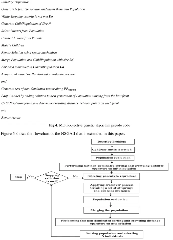
The multi-objective genetic algorithm is one of most widely used and powerful algorithms to solve multi-objective optimization problems and has been proven to be effective in solving various problems. Deb et al. developed the second version of bi-objective genetic algorithm (Deb, Agrawal, Pratap, & Meyarivan, 2000). They studied both quality and variety of Pareto optimal solutions to eliminate the defects of the first version. In this algorithm, two main criteria of quality and order of solutions are followed. Qualified solutions are first selected; if two identical solutions exist, the solution having more order will be selected. The NSGA-II algorithm has two known phases. The first phase uses the ranking criterion and the concept of domination. The second phase which is related to solutions order uses the congestion distance. In the first phase, solutions are ranked, and two values are calculated for each solution: the number of times that a solution is dominated and the number of solutions dominated by the current solution. To determine the two values, all solutions must be compared to each other. If there are solutions with zero number of dominations, these solutions are non-dominated, and they are Pareto optimal.
181 Initialize Population
Generate N feasible solution and insert them into Population While Stopping criteria is not met Do
Generate ChildPopulation of Size N Select Parents from Population Create Children from Parents Mutate Children
Repair Solution using repair mechanism
Merge Population and ChildPopulation with size 2N For each individual in CurrentPopulation Do Assign rank based on Pareto-Fast non-dominates sort end
Generate sets of non-dominated vector along 𝑃𝐹𝑘𝑛𝑜𝑤𝑛
Loop (inside) by adding solution to next generation of Population starting from the best front Until N solution found and determine crowding distance between points on each front end
Report results
Fig 4. Multi-objective genetic algorithm pseudo code Figure 5 shows the flowchart of the NSGAII that is extended in this paper.
182
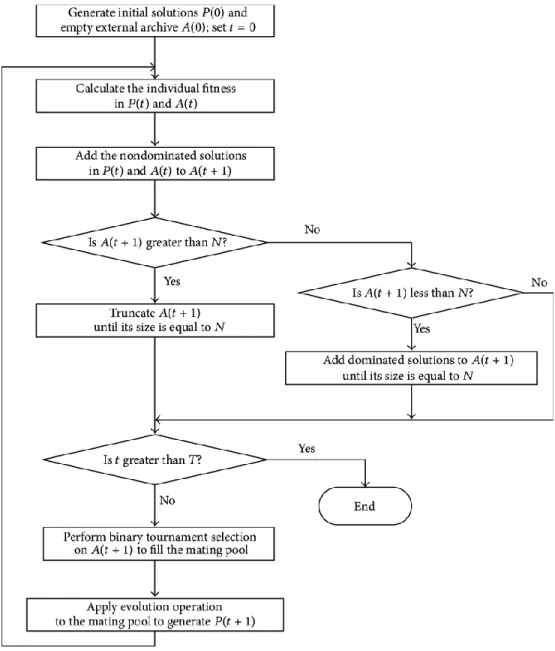
3-3- SPEA-II algorithm
SPEA and SPEA-II are efficient algorithms that use an external archive to store non-dominated solutions found during the search algorithm. SPEA algorithm has some weaknesses in the calculation of strength and fitness, and there was not any secondary criterion for comparison of non-dominated solutions. Hence, Zitzler et al. presented the second version of the algorithm that solved the mentioned weaknesses. The framework of SPEA-II algorithm is described below (Zitzler, Laumanns, & Thiele, 2001).
𝑁𝐸 Maximum archive size of non-dominated solutions E 𝑁𝐹 Population size
K Density computation parameter. (𝐾 = √𝑁𝐸+ 𝑁𝐹)
Step 1: Create initial solutions population 𝑃0 and let 𝐸0= ∅ and 𝑡 = 0.
Step 2: Calculate fitness of each solution i in 𝑃𝑡∪ 𝐸𝑡 as follows.
Sub-step 2-1: Firstly, calculate raw fitness of solution i as follows.
(39) 𝑅(𝑖) = ∑ 𝑠(𝑗)
𝑗∈𝑃𝑡
, ∀ 𝑗 > 𝑖 ∈ 𝑃𝑡,
Where 𝑗 > 𝑖 means that solution j dominates solution i. Moreover, s(j) shows strength value of solution, which is the number of solutions that are dominated by solution j.
Sub-step 2-2: Calculate fitness of solution i as follows.
(40) 𝐷(𝑖) = 1
𝜎𝑖𝑘+ 2, ∀ 𝑖 ∈ 𝑃𝑡,
Where 𝜎𝑖𝑘 is the distance between solution i and the kth nearest neighbor to it.
Sub-step 2-3: Obtain the fitness value by the sum of the raw fitness and the density of solution i, i.e., (41) 𝐹(𝑖) = 𝑅(𝑖) + 𝐷(𝑖), ∀ 𝑖 ∈ 𝑃𝑡.
Step 3: Copy all non-dominated solutions in 𝑃𝑡∪ 𝐸𝑡 to 𝐸t+1. Two possible states may occur.
State 1: If |𝐸𝑡+1| > 𝑁𝐸, |𝐸𝑡+1| − 𝑁𝐸 number of solutions are eliminated by the repetitive method of
deleting the response with the criterion 𝜎𝑘. In fact, the solution that has the minimum distance of 𝜎𝑘 from other solutions is first eliminated. However, if more than one solution has the minimum distance, the second lowest distance can be determined and thus the additional solutions will be deleted similarly (this criterion will cause to delete similar or closely related solutions that do not care about the solutions density).
State 2: If |𝐸𝑡+1| ≤ 𝑁𝐸 , 𝑁𝐸− |𝐸𝑡+1| number of dominated solutions are moved from 𝑃𝑡∪ 𝐸𝑡 to 𝐸𝑡+1 in
183
Step 4: If the stop condition is provided, the algorithm will stop, and it will return |𝐸𝑡+1| solutions.
Step 5: Use the Dual Competition Method to choose parents from set 𝐸𝑡+1.
Step 6: Apply cross-over and mutation operators on parents and produce 𝑁𝑃 children. The children are
added to 𝑃𝑡+1, and one unit will added to the counter (𝑡 = 𝑡 + 1). Then return to step 2.
It should be noted that this algorithm also uses the same method of cross-over and mutation used in the NSGAII algorithm.
Figure 6 shows the flowchart of the SPEAII that is extended in this paper.
184
3-4-PESA-II algorithm
Another of most well-known multi-objective algorithms is the second version of the Pareto-based selection algorithm (PESA-II) which uses genetic algorithm functions to generate new solutions. The first version of this algorithm, presented by (Corne, Jerram, Knowles, & Oates, 2001), had some weaknesses in the selection phase. The developed version of the algorithm, PESA-II, was presented in 2001. Steps of PESA-II algorithm are as follows.
𝑁𝐸 The largest archive of undesirable solutions E. 𝑁𝑃 Population size.
𝑁 Number of networks in each axis of the objective function.
Step 1: Start with a random initial population 𝑃0, set the external archive 𝐸0 to null, and let t = 0.
Step 2: Divide the space into 𝑛𝑘 cloud cubicles where n is the number of networks in each axis of the
objective function, and k is the number of objectives.
Step 3: Combine non-dominated solutions archive 𝐸𝑡 with new solutions of 𝑃𝑡. Three possible states may
occur.
State 1: If a new solution is dominated by at least one of the solutions in archive 𝐸𝑡, delete the new
solution.
State 2: If a new solution dominates several solutions in 𝐸𝑡, delete the dominated solutions from the
archive, add the new solution to archive 𝐸𝑡, and update the cloud cube members.
State 3: If a new solution is not dominated by any solution in 𝐸𝑡 and does not dominate any solution in 𝐸𝑡,
add the solution to 𝐸𝑡. If |𝐸𝑡| = 𝑁𝐸+1, choose an arbitrary cube randomly (the selection is done using the
roulette wheel so that the busy arbitrary cube would be more likely to be selected). Select an available solution randomly and delete it. Finally, update the arbitrary cube members.
Step 4: If the stop criterion is met, stop and show the final 𝐸𝑡.
Step 5: Let 𝑃𝑡 = ∅, combine some solutions of 𝐸𝑡, and select the mutation based on the information
density of the arbitrary cubes. Use the cross-over and mutation to generate 𝑁𝑃 children and copy it to 𝑃𝑡+1.
Step 6: Set t to t + 1 and go to step 3.
It should be noted that this algorithm also uses the same method of cross-over and mutation used in the NSGAII algorithm.
185
Fig 7. Flowchart of the PESAII
4-Comparison of proposed algorithm with mathematical model
After solving the problem by the algorithms coded in Visual C ++ using the Visual Studio system with a 3.2GHz processor, the random-access memory of 4GB in Windows 10 operating system, the obtained results are presented. In this section, to examine the results of the proposed algorithms in comparison with the results of the mathematical model, a number of numerical examples are generated, and the efficiency of the proposed algorithms is evaluated using the MID index. In this index, the Euclidean distance between the final non-dominated solutions generated by the algorithm and the optimal Pareto set produced by CPLEX is calculated as follows.
(42)
2
1 1
max min ,
obj j j
n Q
i best
j j
i j
f f
f f
MID
186
Where 𝑓𝑖𝑗 represents the jth objective value of the ith solution. In addition, 𝑓𝑏𝑒𝑠𝑡𝑗 is the ideal point of the
jth objective function. 𝑓𝑚𝑎𝑥𝑗 and 𝑓𝑚𝑖𝑛 𝑗
are respectively the highest and the lowest values of all Pareto solutions for the jth objective function. |𝑄| and 𝑛𝑜𝑏𝑗 are respectively the number of points in the Pareto
optimal front and the number of objective functions. Since the optimal front is different from that of the algorithm, there is no regularity. Therefore, in this formulation, each member of the algorithm front is calculated with that of the optimal front.
Table 2. Comparison of results of the mathematical model and the proposed algorithm 𝛤1 =|𝐽1|
5 𝑎𝑛𝑑 𝛤2 = |𝐽1|
5 𝛤1 =|𝐽1|
3 𝑎𝑛𝑑 𝛤2 = |𝐽1|
3 𝛤1 =|𝐽1|
2 𝑎𝑛𝑑 𝛤2 = |𝐽2| 2 Instanc es Numbe r Instanc es Size M ID = m ax (𝑁 𝑆 𝐺 𝐴 𝐼𝐼 ,𝑆 𝑃 𝐸 𝐴 ,𝑃 𝐸 𝑆 𝐴 )
Run time (second)
M ID = m ax (𝑁 𝑆 𝐺 𝐴 𝐼𝐼 ,𝑆 𝑃 𝐸 𝐴 ,𝑃 𝐸 𝑆 𝐴 )
Run time (second)
M ID = m ax (𝑁 𝑆 𝐺 𝐴 𝐼𝐼 ,𝑆 𝑃 𝐸 𝐴 ,𝑃 𝐸 𝑆 𝐴 )
Run time (second)
P E S A S P E A N S G A II Cp le x P E S A S P E A N S G A II Cp le x P E S A S P E A N S G A II Cp le x 1.55 72 26 27 167 3.76 41 48 25 162 3.41 50 31 50 153 SM1 Small 1.71 73 43 32 323 4.90 54 79 46 192 3.76 77 37 53 201 SM2 2.61 97 83 69 357 6.52 63 113 121 309 5.74 84 62 72 302 SM3 3.67 100 98 99 341 6.64 70 175 125 326 8.07 88 170 78 330 SM4 4.43 151 128 108 343 7.46 81 182 133 348 9.75 94 186 89 335 SM5 4.46 168 165 148 358 9.04 251 197 181 363 9.81 167 200 91 337 SM6 5.83 199 168 155 362 12.0 8 280 218 187 368 12.8 3 192 208 117 361 SM7 6.00 202 247 163 311 13.1 2 305 221 200 357 13.2 192 230 162 383 SM8 6.04 208 277 165 322 15.1 8 320 228 243 481 13.2 9 217 233 257 394 SM9 8.57 216 296 178 422 15.4 0 329 236 246 484 18.8 5 238 237 297 447 SM10 9.32 241 306 224 427 17.3 2 341 304 331 501 20.5 265 248 304 549 ME1 Mediu m 9.97 251 343 358 432 17.4 6 346 350 347 519 21.9 3 331 255 315 582 ME2
187
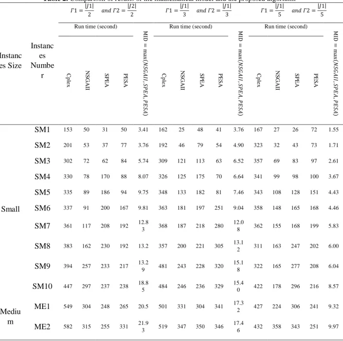
According to the above table, increasing the denominators of 𝜞𝟏 and 𝜞𝟐fractions results in significant changes of running time. Its reason is that the number of constraints is reduced if the level of uncertainty parameters is decreased. Figures 8, 9 and 10 show these changes.
Fig 8. The comparison of running time in Γ1=|J1|/2 and Γ2=|J2|/2
Fig 9. The comparison of running time in Γ1=|J1|/3 and Γ2=|J1|/3 0
50 100 150 200 250 300 350
1 2 3 4 5 6 7 8 9 10 11 12
PESA SPEA NSGAII
0 50 100 150 200 250 300 350 400
1 2 3 4 5 6 7 8 9 10 11 12
188
Fig 10. The amount of solving time for Γ1=|J1|/5 and Γ2=|J1|/5
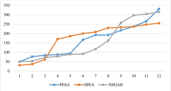
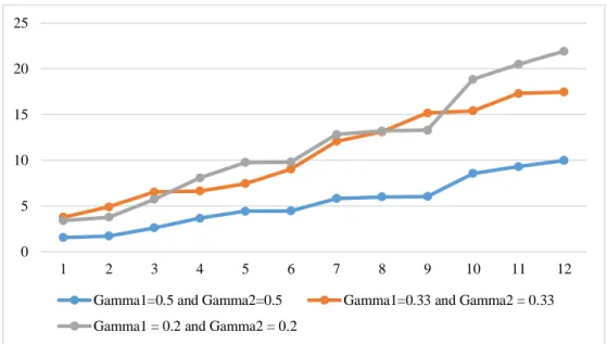
As can be seen, the reduction of uncertainty level in the above figures yields that the algorithms’ times are closer to each other, and the reason is reducing the solving space and consequently, decreasing the number of computations in different repetitions. Therefore, one cannot rank the algorithms from the aspect of their running time; however, decreasing the amount of uncertainty leads to the reduction of MID value, and consequently the obtained solutions of different instances become closer to the exact solutions produced by CPLEX. Figure 8 displays the trend of these changes.
Fig 11. The change of MID values for different values of Γ1 and Γ2
0 50 100 150 200 250 300 350 400
1 2 3 4 5 6 7 8 9 10 11 12
PESA SPEA NSGAII
0 5 10 15 20 25
1 2 3 4 5 6 7 8 9 10 11 12
Gamma1=0.5 and Gamma2=0.5 Gamma1=0.33 and Gamma2 = 0.33 Gamma1 = 0.2 and Gamma2 = 0.2
189
According to figure 11, it can be seen that solutions produced with Γ1 =|J1|
5 and Γ2 = |J1|
5 are closer to
the solutions produced by CPLEX which is due to the small number of uncertain parameters, solving space reduction, and decreasing the number of calculations per iteration. In conclusion, one cannot choose an algorithm as the best to solve real-world problems. In other words, obtained results of small-size instances are similar to CPLEX results. To investigate behavior of the proposed algorithms in larger-dimensional problems, a number of numerical examples with different uncertainty level are generated, and the obtained results are examined in the next section.
5-Evaluation of the proposed algorithms efficiency
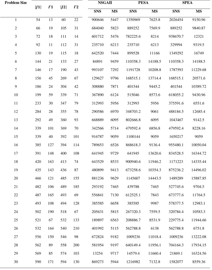
To evaluate the efficiency of the proposed algorithms regarding generation of appropriate solutions, 10 small-size examples, 10 medium-size examples, and 10 large-size examples are generated and compared using the Spread of Non-Domination Solution (SNS) (Maghsoudlou, Kahag, Niaki, & Pourvaziri, 2016) and Maximum Spread (MS) (Samadi, Mehranfar, Fathollahi Fard, & Hajiaghaei-Keshteli, 2018). The SNS and MS indices are calculated as follows:
(43)
2
1 1
1
,
obj n Q
j i
i
MID
jf
SNS
Q
(44)
21
n
obj maxj
minj.
j
MS
f
f
According to table 3, it can be clearly seen that the SPEA algorithm has larger values of SNS and MS criteria which indicates the higher efficiency of this algorithm than the other proposed algorithms; therefore, to solve large-scale problems, it is convenient to use this Algorithm.
190
Table 3. Results of sensitivity analysis of the robustness parameter
Problem Size
Robust Parameters Results
|𝑱𝟏| 𝜞𝟏 |𝑱𝟐| 𝜞𝟐
NSGAII PESA SPEA
SNS MS SNS MS SNS MS
1 54 13 60 22 900646 5447 1350969 7625.8 2026454 9150.96 2 66 19 105 31 684040 5823 889252 7569.9 889252 9840.87 3 72 18 111 14 601712 5476 782225.6 8214 938670.7 12321 4 92 11 112 31 235710 6213 235710 6213 329994 9319.5 5 130 19 115 18 642520 7444 899528 11166 1349292 16749 6 144 21 133 27 84891 9459 110358.3 14188.5 110358.3 14188.5 7 146 17 190 43 993107 7292 1191728 10208.8 1787593 11229.68 8 156 45 269 67 129627 9796 168515.1 13714.4 168515.1 20571.6 9 186 24 304 42 308880 7871 401544 9445.2 401544 10389.72 10 199 59 339 71 367890 6124 515046 8573.6 618055.2 9430.96 11 233 30 347 79 312993 5956 312993 5956 375591.6 6551.6 12 284 28 355 78 290586 6970 348703.2 9061 488184.5 12685.4 13 292 49 360 93 668889 6095 802666.8 6095 1043467 9142.5 14 339 101 369 70 342566 5714 479592.4 6856.8 479592.4 8228.16 15 339 40 392 101 916787 9059 1100144 9059 1650217 9059 16 385 127 394 114 789653 6526 868618.3 9136.4 955480.1 10050.04 17 391 148 400 108 641945 9729 641945 13620.6 834528.5 16344.72 18 420 163 413 74 643529 8533 900940.6 11946.2 1171223 14335.44 19 435 143 436 87 480899 9413 673258.6 10354.3 875236.2 14496.02 20 466 121 485 155 881236 9629 1145607 14443.5 1489289 15887.85 21 482 106 489 185 293192 7465 439788 7465 527745.6 9704.5 22 487 165 493 69 556841 7130 612525.1 7843 673777.6 11764.5 23 493 108 494 128 385585 6658 385585 9987 578377.5 12983.1 24 502 190 518 67 205631 5815 267320.3 7559.5 320784.4 10583.3 25 521 67 532 133 189897 6563 208886.7 8531.9 229775.4 11944.66 26 532 164 540 210 401992 5115 562788.8 6138 562788.8 6751.8 27 556 150 546 98 672824 9182 1009236 11018.4 1009236 13222.08 28 562 89 558 200 581954 9197 640149.4 11956.1 704164.3 17934.15 29 569 85 574 103 13254 9717 14579.4 11660.4 21869.1 16324.56 30 590 171 594 130 869273 5944 1216982 7132.8 1582077 8559.36
191
6-Investigation of case study
In this section, a case study in Iran is investigated. Table 4 and figure 12 show the population and geographical coordinates of the considered basic units in Iran.
b.Graph structure of basic units. a.Basic units structure
Fig 12. Graphical structure of the case study
Since connections between basic units are considered as complete graphs in partitioning problem, the basic units in (a) are converted to the structure of the graph (b). The distance between basic units based on the connections and population of each basic unit are available through the data sets of the Iranian Center for Statistics and other legal geographical information sites. Some data used to solve the problem is presented in table 4.
Table 4. Some information about population, coordinates, and connections between vertices Connectivity Number of inhabitants Centroid Coordinates (x,y) Municipality ID 1022 1021 … 3 2 1 0 0 … 1 1 0 1780 (47.754331,39.042881) 1 0 0 … 1 0 1 41165 (48.53135,37.624719) 2 0 0 … 0 1 1 2841 (48.71865,37.388331) 3 ⋮ ⋮ ⋮ ⋮ ⋮ ⋮ ⋮ ⋮ ⋮ 0 0 … 0 0 0 5417 (49.906411,36.888306) 1021 0 0 … 0 0 0 18756 (50.174514,37.152006) 1022
The following results are the best 10 results of independent implementation of each algorithm. The number of iterations is 200. It is also considered that 𝛤1 =|𝐽1|
2 , 𝛤2 = |𝐽2|
2 , and |𝑃| = 10.
After solving the problem with the SPEA algorithm, which has the best performance, variation interval of the obtained Pareto front are (120, 2506423) and (242, 1031562). Interval of the objective function values are (120, 242) and (2506423, 1031562). The Pareto front structure is considered as figure 13.
192
Fig 13. The Pareto front obtained from solving the SPEA algorithm for the case study
As can be seen, 46 non-dominated Pareto members are generated. To implement the final results in the case study structure, the Pareto member with the first objective function value of 146 and the second objective function value of 2015013 is considered, and the final partitioning is demonstrated in figure 14.
Fig 14. The final partitioning structure of the case study
To analyze sensitivity of the proposed algorithm performance in solving the case study, numerical results for different values of 𝛤1 =|𝐽1|
2 𝛤2 = |𝐽1|
2 , 𝛤1 = |𝐽1|
3 𝛤2 = |𝐽1|
3 , 𝛤1 = |𝐽1|
4 𝛤2 = |𝐽1|
4 , and 𝛤1 = |𝐽1|
5 𝛤2 = |𝐽1|
5 are reported. Table 5 shows the objective function values for each created partitions.
10 12 14 16 18 20 22 24 26
120 140 160 180 200 220 240
O
bj
2
:ba
lan
ce
x
10
5
193
Table 5. The objective function values for the partitions هپ
هن 𝜞𝟏 =
|𝑱𝟏| 𝟐 𝜞𝟐 =
|𝑱𝟏|
𝟐 𝜞𝟏 =
|𝑱𝟏| 𝟑 𝜞𝟐 =
|𝑱𝟏|
𝟑 𝜞𝟏 =
|𝑱𝟏| 𝟒 𝜞𝟐 =
|𝑱𝟏|
𝟒 𝜞𝟏 =
|𝑱𝟏| 𝟓 𝜞𝟐 =
|𝑱𝟏| 𝟓
F1 F2 F1 F2 F1 F2 F1 F2
1 185 1522488 153 1268490 172 1251046 177 1327309
2 198 1450048 149 1336178 152 1299656 197 1374532
3 288 933640 246 847842 243 880579 266 711917
4 275 1855679 202 1441249 210 1346297 237 1570229
5 207 790832 178 654728 152 635829 186 722323
6 301 1507125 286 1367168 258 1288178 259 1181550
7 283 930131 261 829630 260 846349 255 863209
8 282 660395 268 564261 275 541937 255 645863
9 283 1081343 260 988316 223 893226 248 918347
1
0 209 726486 197 663846 186 644481 169 711672
𝑀𝑎𝑥 − 𝑀𝑖𝑛 = 1195284
𝑀𝑎𝑥 − 𝑀𝑖𝑛 = 876988
𝑀𝑎𝑥 − 𝑀𝑖𝑛 = 804360
𝑀𝑎𝑥 − 𝑀𝑖𝑛 = 924366 As can be seen, the more the uncertainty level, the greater the balance in the partitions. It indicates that decreasing the uncertainty level leads to better results in solving the problem. In fact, decision making process becomes more appropriate, and the algorithm will be able to find more qualified solutions. Figure 15 shows the change trend of objective function values for different uncertainty level in all partitions.
Fig 15. The first objective function value obtained from the SPEAII algorithm
140 160 180 200 220 240 260 280 300
0 1 2 3 4 5 6 7 8 9 10
O
B
JE
C
TI
V
E
FU
N
C
TI
O
N
1
194
Fig 16. The second objective function value obtained from the SPEAII algorithm
In figure 16, different signs of ×, the square, the triangle, and + are respectively considered for uncertainty levels of 𝛤1 =|𝐽1|
2 𝛤2 = |𝐽1|
2 , 𝛤1 = |𝐽1|
3 𝛤2 = |𝐽1|
3 , 𝛤1 = |𝐽1|
4 𝛤2 = |𝐽1|
4 , and 𝛤1 = |𝐽1|
5 𝛤2 = |𝐽1|
5 . The uncertainty level 𝛤1 = |𝐽1|
5 𝛤2 = |𝐽1|
5 and 𝛤1 = |𝐽1|
2 𝛤2 = |𝐽1|
2 have respectively the greatest
values in the first and the second objective functions. It can be clearly seen that the lowest difference between the largest and the lowest population of partitions is related to 𝛤1 =|𝐽1|
5 𝛤2 = |𝐽1|
5 which
indicates that better results are obtained from lower level of uncertainty.
7-Conclusions and future suggestions
In this paper, a bi-objective mathematical model is proposed for population partitioning problem under uncertainty conditions. This model can be used as a supporting tool for managers to make final decisions. Since the proposed model is in the category of non-deterministic polynomial hard (NP-hard) problems, meta-heuristic algorithms should be applied to solve real-world problems. Hence, three meta-heuristic algorithms PESA, SPEAII, and NSGAII are proposed. To evaluate the efficiency of the proposed algorithms, suitable comparison criteria are considered.
After investigation of the results, it is found that the SPEAII algorithm has the highest performance level than the other algorithms. The obtained Pareto members are non-dominated. A thorough investigation of one of the produced members confirmed that the optimal structure has complete feasible conditions. Therefore, the results of this model can be used for implementation in real-world conditions. After comparing the proposed algorithms, it can be seen that the NSGAII algorithm results has more distance from the generated front by CPLEX with comparison to the others. This matter suggests that using operators of SPEAII and PESA algorithms can lead to more suitable results.
Comparison of results of different numerical examples reveals that SPEAII algorithm has the highest level of performance and can be used as the final algorithm. In addition, increasing robustness parameter affects the obtained results, and the criterion of the sum of objective functions increases. In other words, more uncertainty results higher level of objective functions and worsen the results. To expand the scope of the research, some suggestions are presented below.
The first suggestion can be implementation of results in larger real-world environments. Investigation of the obtained results can clearly show the performance range of the model and algorithms.
500000 700000 900000 1100000 1300000 1500000 1700000 1900000
0 1 2 3 4 5 6 7 8 9 10
O
B
JE
C
TI
V
E
FU
N
C
T
IO
N
2
195
Using other new meta-heuristic algorithms and comparing the final results can be considered as another research proposal. This can provide a suitable field for generating better solutions by other algorithms as well as comparing the functionality of different algorithms in this problem. Since some parameters of the problem cannot be estimated exactly, using appropriate approaches
to deal with uncertainty will expand the scope of the problem. One of the most credible approaches to deal with uncertainty is robust programming which leads to constructive solutions to changes.
Proposing exact algorithms such as branch and bound and branch and cut can also provide a guarantee for obtaining exact solutions in medium-size and occasionally large-size problems.
References:
Baños, R., Gil, C., Paechter, B., & Ortega, J. (2007). A hybrid meta-heuristic for multi-objective optimization: MOSATS. Journal of Mathematical Modelling and Algorithms, 6(2), 213-230.
Baqir, R. (2002). Districting and government overspending. Journal of political Economy, 110(6), 1318-1354.
Benzarti, E., Sahin, E., & Dallery, Y. (2013). Operations management applied to home care services: Analysis of the districting problem. Decision Support Systems, 55(2), 587-598.
Bertsimas, D., & Sim, M. (2004). The price of robustness. Operations Research, 52(1), 35-53.
Bertsimas, D., & Sim, M. J. M. p. (2003). Robust discrete optimization and network flows. 98(1-3), 49-71.
Bozkaya, B., Erkut, E., & Laporte, G. (2003). A tabu search heuristic and adaptive memory procedure for political districting. European Journal of Operational Research, 144(1), 12-26.
Brooks, S. P., & Morgan, B. J. (1995). Optimization using simulated annealing. Journal of the Royal Statistical Society: Series D (The Statistician), 44(2), 241-257.
Butsch, A., Kalcsics, J., & Laporte, G. (2014). Districting for arc routing. INFORMS Journal on Computing, 26(4), 809-824.
Camacho-Collados, M., Liberatore, F., & Angulo, J. M. (2015). A multi-criteria police districting problem for the efficient and effective design of patrol sector. European Journal of Operational Research, 246(2), 674-684.
Chen, X., & Yum, T.-S. P. (2010). Patrol districting and routing with security level functions. Paper presented at the 2010 IEEE International Conference on Systems, Man and Cybernetics.
Corne, D. W., Jerram, N. R., Knowles, J. D., & Oates, M. J. (2001). PESA-II: Region-based selection in evolutionary multiobjective optimization. Paper presented at the Proceedings of the 3rd Annual Conference on Genetic and Evolutionary Computation.
Datta, D., Figueira, J., Gourtani, A., & Morton, A. (2013). Optimal administrative geographies: an algorithmic approach. Socio-Economic Planning Sciences, 47(3), 247-257.
196
Datta, D., & Figueira, J. R. (2011). Graph partitioning by multi-objective real-valued metaheuristics: A comparative study. Applied Soft Computing, 11(5), 3976-3987.
De Assis, L. S., Franca, P. M., & Usberti, F. L. (2014). A redistricting problem applied to meter reading in power distribution networks. Computers & Operations Research, 41, 65-75.
Deb, K., Agrawal, S., Pratap, A., & Meyarivan, T. (2000). A fast elitist non-dominated sorting genetic algorithm for multi-objective optimization: NSGA-II. Paper presented at the International Conference on Parallel Problem Solving From Nature.
Fan, N., Zheng, Q. P., & Pardalos, P. M. (2012). Robust optimization of graph partitioning involving interval uncertainty. Theoretical Computer Science, 447, 53-61.
García‐Ayala, G., González‐Velarde, J. L., Ríos‐Mercado, R. Z., & Fernández, E. (2016). A novel model for arc territory design: promoting Eulerian districts. International Transactions in Operational Research, 23(3), 433-458.
Garfinkel, R. S., & Nemhauser, G. L. (1970). Optimal political districting by implicit enumeration techniques. Management Science, 16(8), B-495-B-508.
Ghiggi, C., Puliafito, P. P., & Zoppoli, R. (1975). A combinatorial method for health-care districting.
Paper presented at the IFIP Technical Conference on Optimization Techniques.
Kong, Y., Zhu, Y., & Wang, Y. (2018). A center-based modeling approach to solve the districting problem. International Journal of Geographical Information Science, 1-17.
Li, W., Church, R. L., & Goodchild, M. F. (2014). An extendable heuristic framework to solve the p-compact-regions problem for urban economic modeling. Computers, Environment and Urban Systems, 43, 1-13.
Liberatore, F., & Camacho-Collados, M. (2016). A comparison of local search methods for the multicriteria police districting problem on graph. Mathematical Problems in Engineering, 2016.
Lin, H.-Y., & Kao, J.-J. (2008). Subregion districting analysis for municipal solid waste collection privatization. Journal of the Air & Waste Management Association, 58(1), 104-111.
Lin, M., Chin, K.-S., Fu, C., & Tsui, K.-L. (2017). An effective greedy method for the Meals-On-Wheels service districting problem. Computers & Industrial Engineering, 106, 1-19.
Maghsoudlou, H., Kahag, M. R., Niaki, S. T. A., & Pourvaziri, H. (2016). Bi-objective optimization of a three-echelon multi-server supply-chain problem in congested systems: Modeling and solution.
Computers & Industrial Engineering, 99, 41-62.
Minciardi, R., Puliafito, P., & Zoppoli, R. (1981). A districting procedure for social organizations.
European Journal of Operational Research, 8(1), 47-57.
Pezzella, F., Bonanno, R., & Nicoletti, B. (1981). A system approach to the optimal health-care districting. European Journal of Operational Research, 8(2), 139-146.
Ríos-Mercado, R. Z., & López-Pérez, J. F. (2013). Commercial territory design planning with realignment and disjoint assignment requirements. Omega, 41(3), 525-535.
197
Samadi, A., Mehranfar, N., Fathollahi Fard, A., & Hajiaghaei-Keshteli, M. (2018). Heuristic-based metaheuristics to address a sustainable supply chain network design problem. Journal of Industrial and Production Engineering, 35(2), 102-117.
Shirabe, T. (2012). Prescriptive modeling with map algebra for multi-zone allocation with size constraints. Computers, Environment and Urban Systems, 36(5), 456-469.
Steiner, M. T. A., Datta, D., Neto, P. J. S., Scarpin, C. T., & Figueira, J. R. (2015). Multi-objective optimization in partitioning the healthcare system of Parana State in Brazil. Omega, 52, 53-64.
Tran, T.-C., Dinh, T. B., & Gascon, V. (2017). Meta-heuristics to Solve a Districting Problem of a Public Medical Clinic. Paper presented at the Proceedings of the Eighth International Symposium on Information and Communication Technology.
Wang, T., Wu, Z., & Mao, J. (2007). A new method for multi-objective tdma scheduling in wireless sensor networks using pareto-based pso and fuzzy comprehensive judgement. Paper presented at the International Conference on High Performance Computing and Communications.
Zhao, J., Wang, D., & Peng, Q. (2018). Optimizing the Train Dispatcher Desk Districting Problem in
High-Speed Railway Network (No. 18-03607).
Zitzler, E., Laumanns, M., & Thiele, L. (2001). SPEA2: Improving the strength Pareto evolutionary algorithm. TIK-report, 103.