Test Problem Construction for
Single-Objective Bilevel Optimization
Ankur Sinha, Pekka Malo
Department of Information and Service Economy
Aalto University School of Business, Finland
{Firstname.Lastname}@aalto.fi
Kalyanmoy Deb, IEEE Fellow
Department of Mechanical Engineering
Indian Institute of Technology Kanpur, India
[email protected]
KanGAL Report Number 2013002
Abstract
In this paper, we propose a procedure for designing controlled test problems for single-objective bilevel optimization. The proposed procedure is flexible such that the different complexities present in a bilevel problem can be controlled in-dependently of each other. At the same time, the procedure allows to introduce difficulties caused by interaction of the two levels. Using the construction proce-dure, the paper also provides a test suite of twelve test problems, which consists of eight unconstrained and four constrained problems. The test suite contains prob-lems with scalable variables and constraints, which can be used to evaluate the ability of the algorithms in handling bilevel problems. To provide baseline results, we have solved the proposed test problems using a nested bilevel evolutionary al-gorithm. The results can be used for comparison, while evaluating the performance of any other bilevel optimization algorithm.
Keywords:Bilevel optimization, bilevel test-suite, test problem construction, evo-lutionary algorithm.
1
Introduction
Bilevel optimization constitutes a challenging class of optimization problems, where one optimization task is nested within the other. A large number of studies have been conducted in the field of bilevel programming [7, 17, 11, 9], and on its practical appli-cations [2]. Classical approaches commonly used to handle bilevel problems include the Karush-Kuhn-Tucker approach [4, 12], Branch-and-bound techniques [3] and the
use of penalty functions [1]. Despite a significant progress made in classical opti-mization towards solving bilevel optiopti-mization problems, most of these approaches are rendered inapplicable for bilevel problems with higher levels of complexity. Over the last two decades, technological advances and availability of enormous computing re-sources have given rise to heuristic approaches for solving difficult optimization prob-lems. Heuristics such as evolutionary algorithms are recognized as potent tools for handling challenging classes of optimization problems. A number of studies have been performed towards using evolutionary algorithms [19, 18, 9] for solving bilevel prob-lems. However, the research on evolutionary algorithms for bilevel problems is still in nascent stage, and significant improvement in the existing approaches is required. Most of the heuristic approaches lack a finite time convergence proof for optimization problems. Therefore, it is a common practice among researchers to demonstrate the convergence of their algorithms on a test bed constituting problems with various com-plexities. To the best knowledge of the authors, in the domain of single objective bilevel programming, there does not exist a systematic framework for constructing bilevel test problems with controlled difficulties. Test problems, which offer various difficulties found in practical application problems, are often required during the construction and evaluation of algorithms.
Past studies [13] on bilevel optimization have introduced a number of simple test problems. However, the levels of difficulty cannot be controlled in these test problems. In most of the studies, the problems are either linear [14], or quadratic [5, 6], or non-scalable with fixed number of decision variables. Application problems in transporta-tion (network design, optimal pricing), economics (Stackelberg games, principal-agent problem, taxation, policy decisions), management (network facility location, coordina-tion of multi-divisional firms), engineering (optimal design, optimal chemical equilib-ria) etc [10] have also been used to demonstrate the efficiency of algorithms. For most of these problems, the true optimal solution is unknown. Therefore, it is hard to iden-tify, whether a particular solution obtained using an existing approach is close to the optima. Under these uncertainties, it is not possible to systematically evaluate solution procedures on practical problems. These drawbacks pose hurdles in algorithm devel-opment, as the performance of the algorithms cannot be evaluated on various difficulty frontiers. A test-suite with controllable level of difficulties helps in understanding the bilevel algorithms better. It gives an information as to what properties of bilevel prob-lems is being efficiently handled by the algorithm and what is not. An algorithm which performs well on the test problem by effectively tackling most of the challenges of-fered by the test-suite is expected to perform good on other simpler problems as well. Therefore, controlled test problems are necessary for the advancement of the research on bilevel optimization using evolutionary algorithms.
In this paper, we identify the challenges commonly encountered in bilevel opti-mization problems. A test problem construction procedure is proposed, which mimics these difficulties in a controllable manner. Using the construction procedure, we pro-pose a collection of bilevel test problems scalable in terms of variables and constraints. The proposed scheme allows to control the difficulties at the two levels independently of each other. At the same time, it also allows to control the extent of difficulty arising due to interaction of the two levels . The test problems generated using the framework are such that the optimal solution of the bilevel problem is known. Moreover, the
in-duced set of the bilevel problem is known as a function of the upper level variables. Such information helps the algorithm developers to debug their procedures during the development phase, and also allows to evaluate the convergence properties of the ap-proach.
The paper is organized as follows. In the next section, we explain the structure of a general bilevel optimization problem and introduce the notation that is used through-out the paper. Section 3 presents our framework for constructing scalable test problems for bilevel programming. Thereafter, following the guidelines of the construction pro-cedure, we suggest a set of twelve scalable test problems in Section 4. To create a benchmark for evaluating different solution algorithms, the problems are solved using a simple nested bilevel evolutionary algorithm which is a nested scheme described in Section 5. The results for the baseline algorithm are discussed in Section 6.
2
Description of a Bilevel Problem
A bilevel optimization problem involves two levels of optimization tasks, where one level is nested within the other. The outer optimization task is usually called as upper level optimization task, and the inner optimization task is called as lower level opti-mization task. The structure of such an optiopti-mization problem requires that only the optimal solutions of the inner optimization task are acceptable as feasible members for the outer optimization task. The problem contains two types of variables; namely the upper level variablesxu, and the lower level variablesxl. The lower level is opti-mized with respect to the lower level variablesxl, and the upper level variablesxuact as parameters. An optimal lower level vector and the corresponding upper level vec-torxu constitute a feasible upper level solution, provided the upper level constraints are also satisfied. The upper level problem involves all variablesx = (xu,xl), and the optimization is supposed to be performed with respect to bothxuandxl. In the following, we provide two equivalent formulations for a general bilevel optimization problem with one objective at both levels:
Definition 1 (Bilevel Optimization Problem (BLOP)) Let X = XU ×XL denote
the product of the upper-level decision spaceXU and the lower-level decision space
XL, i.e. x = (xu,xl) ∈ X, ifxu ∈ XU and xl ∈ XL. For upper-level objective
functionF :X →Rand lower-level objective functionf :X →R, a general bilevel
optimization problem is given by
Minimize
x∈X
F(x),
s.t. xl∈argmin
xl∈XL
f(x)gi(x)≥0, i∈I ,
Gj(x)≥0, j∈J.
(1)
where the functionsgi : X → R,i ∈ I, represent lower-level constraints andGj :
X→R,j∈J, is the collection of upper-level constraints.
In the above formulation, a vectorx(0) = (x(0)
u ,x
(0)
l )is considered feasible at the upper level, if it satisfies all the upper level constraints, and vectorx(0)l is optimal
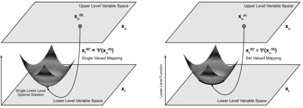
at the lower level for the givenx(0)u . We observe in this formulation that the lower-level problem is a parameterized constraint to the upper-lower-level problem. An equivalent formulation of the bilevel optimization problem is obtained by replacing the lower-level optimization problem with a set value function which maps the given upper-lower-level decision vector to the corresponding set of optimal lower-level solutions. In the domain of Stackelberg games, such mapping is referred as the rational reaction of the follower on the leader’s choicexu.
Definition 2 (Alternative definition of Bilevel Problem) Let set-valued functionΨ :
XU ⇒XL, denote the optimal-solution set mapping of the lower level problem, i.e.
Ψ(xu) = argmin
xl∈XL
f(x)
gi(x)≥0, i∈I . A general bilevel optimization problem (BLOP) is then given by
Minimize
x∈X
F(x),
s.t. xl∈Ψ(xu),
Gj(x)≥0, j∈J.
(2)
where the functionΨmay be a single-vector valued or a multi-vector valued function
depending on whether the lower level function has multiple global optimal solutions or not.
In the test problem construction procedure, theΨfunction provides a convenient description of the relationship between the upper and lower level problems. Figures 1 and 2 illustrate two scenarios, whereΨcan be a single vector valued or a multi-vector valued function respectively. In Figure 1, the lower level problem is shown to be a paraboloid with a single minimum function value corresponding to the set of upper level variablesxu. Figure 2 represents a scenario where the lower level function is a paraboloid sliced from the bottom with a horizontal plane. This leads to multiple min-imum values for the lower level problem, and therefore, multiple lower level solutions correspond to the set of upper level variablesxu.
3
Test Problem Construction Procedure
The presence of an additional optimization task within the constraints of the upper optimization task leads to a significant increase in complexity, as compared to any sin-gle level optimization problem. We identify various kinds of complexities, which a bilevel optimization problem can offer, and provide a test problem construction pro-cedure which can induce these difficulties in a controllable manner. In order to create realistic test problems, the construction procedure should be able to control the scale of difficulties at both levels independently and collectively, such that the performance of algorithms in handling the two levels is evaluated. The test problems created using the construction procedure are expected to be scalable in terms of number of decision variables and constraints, such that the performance of the algorithms can be evaluated
Figure 1: Relationship between upper and lower level variables in case of a single-vector valued mapping. For simplicity the lower level function is in the shape of a paraboloid.
Figure 2: Relationship between upper and lower level variables in case of a multi-vector valued mapping. The lower level function is shown in the shape of a paraboloid with the bottom sliced with a plane.
against increasing number of variables and constraints. The construction procedure should be able to generate test problems with the following properties:
Necessary Properties:
1. The optimal solution of the bilevel optimization should be known.
2. Clear identification of a relationship between the lower level optimal solutions and the upper level variables.
Properties for inducing difficulties:
1. Controlled difficulty in convergence at upper and lower levels. 2. Controlled difficulty caused by interaction of the two levels.
3. Multiple global solutions at the lower level for a given set of upper level vari-ables.
4. Possibility to have either conflict or cooperation between the two levels. 5. Scalability to any number of decision variables at upper and lower levels. 6. Constraints (preferably scalable) at upper and lower levels.
Next, we provide the bilevel test problem construction procedure, which is able to induce most of the difficulties suggested above.
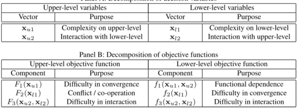
Table 1: Overview of test-problem framework components
Panel A: Decomposition of decision variables
Upper-level variables Lower-level variables
Vector Purpose Vector Purpose
xu1 Complexity on upper-level xl1 Complexity on lower-level
xu2 Interaction with lower-level xl2 Interaction with upper-level
Panel B: Decomposition of objective functions
Upper-level objective function Lower-level objective function
Component Purpose Component Purpose
F1(xu1) Difficulty in convergence f1(xu1,xu2) Functional dependence
F2(xl1) Conflict / co-operation f2(xl1) Difficulty in convergence
F3(xu2,xl2) Difficulty in interaction f3(xu2,xl2) Difficulty in interaction
3.1
Objective functions in the test-problem framework
To create a tractable framework for test-problem construction, we split the upper and lower level functions into three components. Each of the components is specialized for induction of certain kinds of difficulties into the bilevel problem. The functions are determined based on the required complexities at upper and lower levels independently, and also by the required complexities because of the interaction of the two levels. We write a generic bilevel test problem as follows:
F(xu,xl) =F1(xu1) +F2(xl1) +F3(xu2,xl2) f(xu,xl) =f1(xu1,xu2) +f2(xl1) +f3(xu2,xl2) where
xu= (xu1,xu2) and xl= (xl1,xl2)
(3)
In the above equations, each of the levels contains three terms. A summary on the roles of different terms is provided in Table 1. The upper level and lower level variables have been broken into two smaller vectors (see Panel A in Table 1). The vectorsxu1 and xl1 are used to induce complexities at the upper and lower levels independently. The vectorsxu2andxl2are responsible to induce complexities because of interaction. In a similar fashion, we decompose the upper and lower level functions such that each of the components is specialized for a certain purpose only (see Panel B in Table 1). At the upper level, the termF1(xu1)is responsible for inducing difficulty in convergence solely at the upper level. Similarly, at the lower level, the termf2(xl1) is responsible for inducing difficulty in convergence solely at the lower level. The term F2(xl1) decides if there is a conflict or a cooperation between the upper and lower levels. The termsF3(xl2,xu2)andf3(xl2,xu2)are interaction terms which can be used to induce difficulties because of interaction at the two levels. TermF3(xl2,xu2) may also induce a cooperation or a conflict. Finally,f1(xu1,xu2)is a fixed term for the lower level optimization problem and does not induce any convergence difficulties. It is used along with the lower level interaction term to create a functional dependence between lower level optimal solution(s) and the upper level variables. The difficulties related to constraints are handled separately.
3.1.1 Controlled difficulty in convergence
The test-problem framework allows to introduce difficulties in terms of convergence at both levels of bilevel optimization problem while retaining sufficient control. To demonstrate this, let us consider the structure of the lower level minimization problem.
For a givenxu= (xu1,xu2), the lower level minimization problem is written as
Min (xl1,xl2)
f(xu,xl) =f1(xu1,xu2) +f2(xl1) +f3(xu2,xl2),
where the upper level variables(xu1,xu2)act as parameters for the optimization prob-lem. The corresponding optimal-set mapping is given by
Ψ(xu) = argmin{f2(xl1) +f3(xu2,xl2) :xl∈XL},
wheref1does not appear due to its independence fromxl. Since all of the terms are independent of each other, we note that the optimal value of the functionf can be recovered by optimizing the functionsf2 andf3 individually. Functionf2 contains only lower level variables xl1, which do not interact with upper level variables. It introduces convergence difficulties at the lower level without affecting the upper level optimization task. Functionf3contains both lower level variablesxl2, and upper level variablesxu2. The optimal value of this function depends onxu2.
The following example shows that the calibration of the desired difficulty level for the lower level problem boils down to the choice of functionsf2andf3such that their optima are known.
Example 1: To create a simple lower level function, let the dimension of the
vari-able sets be as follows: dim(xu1) = U1, dim(xu2) = U2, dim(xl1) = L1 and
dim(xl2) = L2. Consider a special case whereL2 =U2, then the three functions
could be defined as follows:
f1(xu1,xu2) =P
U1 i=1(x
i u1)
2+PU2
i=1(x i u2)
2
f2(xl1) =P
L1 i=1(x
i l1)
2 f3(xu2,xl2) =P
U2 i=1(x
i
u2−x
i l2)
2
wheref1affects only the value of the function without inducing any convergence dif-ficulties. The corresponding optimal set mappingΨis reduced to an ordinary vector valued function
Ψ(xu) ={(xl1,xl2) :xl1=0,xl2=xu2}.
As discussed above, other functions can be chosen with desired complexities to induce difficulties at the lower level and come up with a variety of lower level func-tions. Similarly,F1is a function ofxu1, which does not interact with any lower level variables. It causes convergence difficulties at the upper level without introducing any other form of complexity in the bilevel problem.
3.1.2 Controlled difficulty in interaction
Next, we consider difficulties due to interaction between the upper and lower level optimization tasks. The upper level optimization task is defined as a minimization
problem over the graph of the optimal solution set mappingΨ, i.e.
Min{F(xu,xl) :xl∈Ψ(xu),xu∈XU}
where the objective function
F(xu,xl) =F1(xu1) +F2(xl1) +F3(xu2,xl2)
is a sum of three independent terms. Our primary interest is on the last two terms F2(xl1)andF3(xu2,xl2), which determine the type of interaction there is going to be between the optimization problems. This can be done in two different ways, depending on whether a cooperation or a conflict is desired between the upper and lower level problems.
Definition 3 (Co-operative bilevel test-problem) A bilevel optimization problem is
said to be co-operative, if in the vicinity ofx∗l for a particularxu, an improvement
in the lower level function value leads to an improvement in the upper level function value. Within our test problem framework, the independence of terms in the upper level
objective functionF implies that the co-operative condition is satisfied when for any
upper level decisionxuthe corresponding lower level decisionxl= (xl1,xl2)is such
thatxl1 ∈ argmin{F2(xl1) : xl ∈ Ψ(xu)}andxl2 ∈ argmin{F3(xu2,xl2) : xl ∈
Ψ(xu)}.
Definition 4 (Conflicting bilevel test-problem) A bilevel optimization problem is said
to be conflicting, if in the vicinity ofx∗l for a particularxu, an improvement in the
lower-level function value leads to an adverse effect on the upper level function value. In our framework, a conflicting test problem is obtained when for any upper level
de-cisionxu the corresponding lower level decision xl = (xl1,xl2)is such thatxl1 ∈
argmax{F2(xl1) :xl∈Ψ(xu)}andxl2∈argmax{F3(xu2,xl2) :xl∈Ψ(xu)}.
In the above general form, the functionsf2andf3may have multiple optimal solu-tions for any given upper level decisionxu. However, in order to create test problems with tractable interaction patterns, we would like to define them such that each problem has only a single lower lower level optimum for a givenxu. To ensure the existence of single lower level optimum, and to enable realistic interactions between the two levels, we consider imposing the following simple restrictions on the objective functions:
Case 1. Creating co-operative interaction: A test problem with co-operative
in-teraction pattern can be created by choosing
F2(xl1) = f2(xl1) (4)
F3(xu2,xl2) = F4(xu2) +f3(xu2,xl2),
whereF4(xu2)is any function ofxu2whose minimum is known.
Case 2. Creating conflicting interaction: A test problem with a conflict between
right hand side in (4):
F2(xl1) = −f2(xl1) (5)
F3(xu2,xl2) = F4(xu2)−f3(xu2,xl2).
The choice ofF2andF3suggested here is a special case, and there can be many other ways to achieve conflict or co-operation using the two functions.
Case 3. Creating mixed interaction: There may be a situation of both cooperation
and conflict if functionsF2andF3are chosen with opposite signs as,
F2(xl1) = f2(xl1) (6)
F3(xu2,xl2) = F4(xu2)−f3(xu2,xl2) or
F2(xl1) = −f2(xl1) (7)
F3(xu2,xl2) = F4(xu2) +f3(xu2,xl2).
Example 2: Consider a bilevel optimization problem where the lower level task
is given by Example 1. According to the above procedures, we can produce a test problem with a conflict between the upper and lower level by defining the upper level objective function as follows:
F1(xu1) =P
U1 i=1(x
i u1)2
F2(xl1) =−P
L1 i=1(x
i l1)
2 F3(xu2,xl2) =−P
U2 i=1(x
i
u2−xil2) 2.
(8)
The chosen formulation corresponds to Case 2, whereF4(xu2) = 0. The final optimal solution of the bilevel problem isF(xu,xl) = 0for(xu,xl) =0.
3.1.3 Multiple Global Solutions at Lower Level
In this sub-section, we discuss about constructing test problems with lower level func-tion having multiple global solufunc-tions for a given set of upper level variables. To achieve this, we formulate a lower level function which has multiple lower level optima for a givenxu, such thatx∗l ∈Ψ(xu). Then, we ensure that out of all these possible lower level optimal solutions, one of them (x∗∗l ) corresponds to the best upper level function value, i.e.,
x∗∗l ∈argmin x∗
l
F(xu,x∗l)
x∗l ∈Ψ(xu) (9)
To incorporate this difficulty in the problem, we choose the second functions at the upper and lower levels. Given that the term f2(xl1) is responsible for causing complexities only at the lower level, we can freely formulate it such that it has multiple lower level optimal solutions. From this it necessarily follows that the entire lower level function has multiple optimal solutions.
Example 3: We describe the construction procedure by considering a simple ex-ample, where the cardinalities of the variables are,dim(xu1) = 2,dim(xu2) = 2,
dim(xl1) = 2anddim(xl2) = 2, and the lower level function is defined as follows,
f1(xu1,xu2) = (x1u1)2+ (x2u1)2+ (x1u2)2+ (x2u2)2 f2(xl1) = (x1l1−x
2 l1)
2 f3(xu2,xl2) = (x1u2−x1l2)
2+ (x2
u2−x2l2) 2
(10)
Here, we observe thatf2(xl1)induces multiple optimal solutions, as its minimum value is0for allx1
l1 =x
2
l1. At the minimumf3(xu2,xl2)fixes the values ofx1l2andx 2 l2to x1
u2andx2u2respectively. Next, we write the upper level function ensuring that out of the setx1
l1=x2l1, one of the solutions is best at upper level. F1(xu1) = (x1u1)2+ (x2u1)2
F2(xl1) = (x1l1) 2+ (x2
l1) 2
F3(xu2,xl2) = (x1u2−x2l2)2+ (x2u2−x2l2)2
(11)
The formulation of F2(xl1), as sum of squared terms ensures that x1l1 = x2l1 = 0 provides the best solution at the upper level for any given(xu1,xu2).
3.2
Difficulties induced by constraints
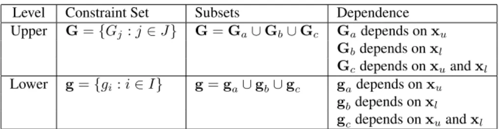
In this subsection, we discuss about the types of constraints which can be encoun-tered in a bilevel optimization problem. We only consider inequality constraints in this bilevel test problem construction framework. Considering that the bilevel problems have the possibility to have constraints at both levels, and each constraint could be a function of two different kinds of variables, the constrained set at both levels can be further broken down into smaller subsets as follows:
Level Constraint Set Subsets Dependence
Upper G={Gj :j∈J} G=Ga∪Gb∪Gc Gadepends onxu Gbdepends onxl Gcdepends onxuandxl Lower g={gi:i∈I} g=ga∪gb∪gc gadepends onxu
gbdepends onxl gcdepends onxuandxl
Table 2: Composition of the constraint sets at both levels.
In Table 2, Gandg denote the set of constraints at the upper and lower level respectively. Each of the constraint set can be broken into three smaller subsets, as shown in the table. The first subset represents constraints that are functions of the upper level variables only, the second subset represents constraints that are functions of lower level variables only, and the third subset represents constraints that are functions of both upper and lower level variables. The reason for splitting the constraints into smaller subsets is to develop an insight for solving these kinds of problems using an
evolutionary approach. If the first constraint subset (Gaorga) is non-empty at either of the two levels, then for any givenxuwe should check the feasibility of constraints in the setsGaandga, before solving the lower level optimization problem. In case, there is one or more infeasible constraints inga, then the lower level optimization problem does not contain optimal lower level solution (x∗l) for the givenxu. However, if one or more constraints are infeasible withinGb, then a lower level optimal solution (x∗l) may exist for the givenxu, but the pair (xu,x∗u) will be infeasible for the bilevel problem. Based on this property, a decision can be made, whether it is useful to solve the lower level optimization problem at all for a givenxu.
The upper level constraint subsets, Gb depends onxl, and Gc depends on xu andxl. The values from these constraints are meaningful only when the lower level vector is an optimal solution to the lower level optimization problem. Based on the various constraints which may be functions ofxu, or xl or both, a bilevel problem introduces different kinds of difficulties in the optimization task. In this paper, we aim to construct such kinds of constrained bilevel test problems which incorporate some of these complexities. We have proposed four constrained bilevel problems, each of which has at least one or more of the following properties,
1. Constraints exist, but are not active at the optimum
2. A subset of constraints, or all the constraints are active at the optimum
3. Upper level constraints are functions of only upper level variables, and lower level constraints are functions of only lower level variables
4. Upper level constraints are functions of upper as well as lower level variables, and lower level constraints are also functions of upper as well as lower level variables
5. Lower level constraints lead to multiple global solutions at the lower level 6. Constraints are scalable at both levels
While describing the test problems in the next section, we discuss the construction procedure for the individual constrained test problems.
4
SMD test problems
By adhering to the design principles introduced in the previous section, we now pro-pose a set of twelve problems which we call as the SMD test problems. Each problem represents a different difficulty level in terms of convergence at the two levels, com-plexity of interaction between two levels and multi-modalities at each of the levels. The first eight problems are unconstrained and the remaining four are constrained.
u2
with respect to lower level variables with respect to upper level variables
u2 u1
at (x ,x ) = (−2,−2) U: Lower level function contours with respect to lower level variables
l2 l1 l2 l1 x x x x x x x l2 l1 x x u1
with respect to lower level variables
u2
x u2 u1
at (x ,x ) = (0,0) S: Lower level function contours with respect to lower level variables
l1
x
l2
x
l1
R: Lower level function contours
at (x ,x ) = (2,2)u1 u2
Q: Lower level function contours
at (x ,x ) = (2,−2)u1 u2 P: Upper level function contours
at optimal lower level variables with respect to lower level variables
T: Lower level function contours
at (x ,x ) = (−2,2)u1
l2 4.3 4.1 4.3 4.5 5 5.5 5 11 4.5 4.3 4.1 15 15 1.5 1 0.5 0.1 5.5 500 20 30 8 1 4 500 100 500 100 4.1 4.5 5 5.5 11 5.5 4.5 4.3 4.1 4.5 5 5.5 11 5.5 4.5 4.3 11 5 5.5 5 100 100 500 5.5 4.3 −0.4
−1 −0.5 0 0.5 1 1.5−1.5 −1 −0.5 0 0.5 1 1.5
−0.2 0 0.2
−0.4 −0.2 0 0.2 0.4 0.6
0.8 1 1.2 1.4 1.6 0.4−1.6 −1.4 −1.2 −1 −0.8 −0.6 1.6 1.4 1.2
−4 −2 0 2 4
−4 −2 0 2 4 −0.2 −0.4 1 −0.6 0 0.4 0.8 0.6 0.4 −1.6 0.2 −1.4 −1.2
−0.4 −0.2 0 0.2 −1 −0.8 −1.5
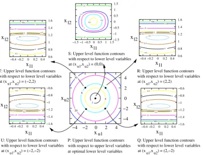
Figure 3: Upper and lower level function contours for a four-variable SMD1 test prob-lem.
4.1
SMD1
This is a simple test problem where the lower level problem is a convex optimization task, and the upper level is convex with respect to upper level variables and optimal lower level variables. The two levels cooperate with each other.
F1=P
p i=1(x
i u1)2
F2=P
q i=1(x
i l1)
2
F3=P
r i=1(x
i u2)2+
Pr
i=1(x i
u2−tanxil2) 2
f1=P
p i=1(x
i u1)2
f2=P
q i=1(x
i l1)2
f3=Pri=1(xui2−tanxil2)2
(12)
The range of variables is as follows, xi
u1∈[−5,10], ∀ i∈ {1,2, . . . , p}
xi
u2∈[−5,10], ∀ i∈ {1,2, . . . , r}
xi
l1∈[−5,10], ∀ i∈ {1,2, . . . , q}
xi l2∈(−
π 2 ,
π
2), ∀ i∈ {1,2, . . . , r}
(13)
Relationship between upper level variables and lower level optimal variables is given as follows,
xi
l1= 0, ∀ i∈ {1,2, . . . , p}
xi
l2= tan−1xiu2, ∀ i∈ {1,2, . . . , r}
P: Upper level function contours at optimal lower level variables with respect to upper level variables
Q: Upper level function contours at (x ,x ) = (2,−2)u1 u2
with respect to lower level variables with respect to lower level variables
S: Upper level function contours at (x ,x ) = (0,0)u1 u2
with respect to lower level variables R: Upper level function contours at (x ,x ) = (2,2)u1 u2 with respect to lower level variables
T: Upper level function contours at (x ,x ) = (−2,2)u1 u2
with respect to lower level variables U: Upper level function contours at (x ,x ) = (−2,−2)u1 u2
xu1 xu2 xl1 x l2 xl1 l2 l1 l2 x x x x x x x l1 l2 l1 l2 8.1 8.5 8.5 9 9.5 9.5 9 15 100 500 8.1 8.5 9 9.5 8.5 500 100 9 9.5 15 8.1 8.5 9 9.5 8.5 500 100 9 9.5 15 20 30 8 1 4 0.1 0.5 1 1.5 15 15 8.5 8.5 9 9.5 9.5 9 15 100 500 8.1
−0.4 −0.2 0 0.2 0.4−1.6 −1.4 −1.2 −1 −0.8 −0.6 −0.4 −0.2 0 0.2 0.4 0.6 0.8 1 1.2 1.4 1.6
−0.4 −0.2 0 0.2 0.4 0.6 0.8 1 1.2 1.4 1.6
−4 −2 0 2 4
−4 −2 0 2 4 −1.5 −1 −0.5 0 0.5 1 1.5−1.5
−1 −0.5 0 0.5 1 1.5
−0.4 −0.2 0 0.2 0.4 −1.6 −1.4 −1.2 −1 −0.8 −0.6
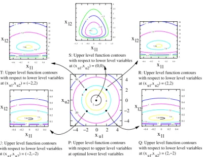
Figure 4: Upper level function contours for a four-variable SMD1 test problem.
The values of the variables at the optima arexu = 0andxlis obtained by the rela-tionship given above. Both the upper and lower level functions are equal to zero at the optima.
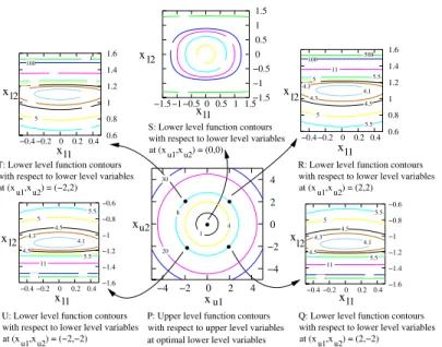
Figure 3 shows the contours of the upper and lower level functions with respect to the upper and lower level variables for a four-variable test problem. The problem has two upper level variables and two lower level variables, such that the dimensions of xu1,xu2,xl1andxu2are all one. Sub-figure P shows the upper level function contours with respect to the upper level variables, assuming that the lower level variables are at the optima. Fixing the upper level variables(xu1,xu2)at five different locations, i.e. (2,2),(−2,2),(2,−2),(−2,−2)and(0,0), the lower level function contours are shown with respect to the lower level variables. This shows that the contours of the lower level optimization problem may be different for different upper level vectors.
Figure 4 shows the contours of the upper level function with respect to the up-per and lower level variables. Sub-figure P once again shows the upup-per level func-tion contours with respect to the upper level variables. However, sub-figures Q, R, S, T and V now represent the upper level function contours at different(xu1,xu2), i.e. (2,2),(−2,2),(2,−2),(−2,−2)and(0,0). From sub-figures Q, R, S, T and V, we observe that if the lower level variables move away from its optimal location, the up-per level function value deteriorates. This means that the upup-per level function and the lower level functions are cooperative.
P: Upper level function contours
at (x ,x ) = (2,−2)u1 u2
with respect to lower level variables u2 x x l2 l1 l2 l1
at optimal lower level variables with respect to upper level variables with respect to lower level variables S: Lower level function contours at (x ,x ) = (0,0)u1 u2
with respect to lower level variables R: Lower level function contours at (x ,x ) = (2,2)u1 u2
with respect to lower level variables U: Lower level function contours at (x ,x ) = (−2,−2)u1 u2
with respect to lower level variables T: Lower level function contours at (x ,x ) = (−2,2)
l2 l1 x x x u1 u2 x xl2 l1 x l2 x l1 x x u1 x
Q: Lower level function contours 4.1 4.5 5 5.5 7.5 5 5.5 4.01 4.1 4.5 5 5.5 7.5 5 5.5 4.01 0.1 0.5 1.5 1 5.5 5 4.1 20 8 1 4 30 4.1 5 5.5 4.01 4.5 5 4.5 4.01 4.5 5 4.5 20
−0.2 0 0.2 0.4 0.1 0.2 0.4 0.1 0.2 0.3 0.4 0.5 0.6 0.3 0.4 0.5 0.6
−4 −2 0 2 4
−4 −2 6 0 4 2 0.4 4 0.2 −1.5 −1 −0.5 0 0.5 1 1.5
0.5 1 1.5 2 2.5 3 3.5 4 20 18 16 14 12 10 8 0 −0.2 −0.4 2
−0.4 −0.2 0 0.2 −0.4
−0.4 −0.2 0 0.2 0.4 2 4 6 8 10 12 14 16 18
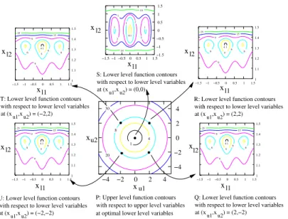
Figure 5: Upper and lower level function contours for a four-variable SMD2 test prob-lem.
4.2
SMD2
This test problem is similar to the SDM1 test problem, however there is a conflict between the upper level and lower level optimization task. The lower level optimization problem is once again a convex optimization task and the upper level optimization is convex with respect to upper level variables and optimal lower level variables. Since, the two levels are conflicting, an inaccurate lower level optimum may lead to upper level function value better than the true optimum for the bilevel problem.
F1=P
p i=1(x
i u1)2
F2=−P
q i=1(x
i l1)
2
F3=P
r i=1(x
i u2)2−
Pr
i=1(x i
u2−logxil2) 2
f1=P
p i=1(x
i u1)2
f2=P
q i=1(x
i l1)
2
f3=Pri=1(xui2−logxil2)2
(15)
The range of variables is as follows, xi
u1∈[−5,10], ∀ i∈ {1,2, . . . , p}
xi
u2∈[−5,1], ∀ i∈ {1,2, . . . , r}
xi
l1∈[−5,10], ∀ i∈ {1,2, . . . , q}
xi
l2∈(0, e], ∀ i∈ {1,2, . . . , r}
P: Upper level function contours at optimal lower level variables with respect to upper level variables
Q: Upper level function contours at (x ,x ) = (2,−2)u1 u2
with respect to lower level variables with respect to lower level variables
S: Upper level function contours at (x ,x ) = (0,0)u1 u2
with respect to lower level variables R: Upper level function contours at (x ,x ) = (2,2)u1 u2
with respect to lower level variables U: Upper level function contours at (x ,x ) = (−2,−2)u1 u2
with respect to lower level variables T: Upper level function contours at (x ,x ) = (−2,2)u1 u2
xu1 x xl1 x l2 xl1 l2 x x x x x l1 l2 l1 l2 l1 l2 x x u2 7.9 7.5 7 6.5 7.5 7 6.5 7.99 7.9 7.5 7 6.5 7.5 7 6.5 7.99 6.5 7 7.5 7.9 7.99 7.5 7 −1 −1.5 −0.5 −0.1 7 6.5 7.99 7.5 7 7.5 7.9 20 8 1 4 30
−0.4 −0.2 0 0.2 0.4 0.1 0.2 0.3 0.4 0.5 0.6
−0.4 −0.2 0 0.2 0.4 0.1 0.2 0.3 0.4 0.5 0.6
−0.4 −0.2 0 0.2 0.4 2 4 6 8 10 12 14 16 18 20
−1.5 −1 −0.5 0 0.5 1 1.5 0.5 1 1.5 2 2.5 3 3.5 4
−0.4 −0.2 0 0.2 0.4 2 4 6 8 10 12 14 16 18 20
−4 −2 0 2 4 −4 −2 0 2 4
Figure 6: Upper level function contours for a four-variable SMD2 test problem.
Relationship between upper level variables and lower level optimal variables is given as follows,
xil1= 0, ∀ i∈ {1,2, . . . , q}
xil2= log−1xiu2, ∀ i∈ {1,2, . . . , r}
(17) The values of the variables at the optima arexu = 0andxlis obtained by the rela-tionship given above. Both the upper and lower level functions are equal to zero at the optima.
Figure 5 shows the contours of the upper and lower level functions with respect to the upper and lower level variables for a four-variable test problem. The problem has two upper level variables and two lower level variables, such that the dimension ofxu1,xu2,xl1andxu2are all one. The figure provides the same information about SMD2, as Figure 3 provides about SMD1. However, the shape of the contours differ, which is caused by the use of differentF3andf3functions.
Figure 6 shows the contours of the upper level function with respect to the upper and lower level variables, and provides the same information as Figure 4 provides about SMD1. This figure shows the conflicting nature of the problem caused by using a negative sign inF2. The conflicting nature can be observed from the sub-figures Q, R, S, T and U. For a givenxu, as one moves away from the lower level optimal solution, the upper level function value further reduces. On the other hand, in 5 we observe that moving away from the lower level optimal solution causes an increase in lower level function value.
4.3
SMD3
In this test problem there is a cooperation between the two levels. The difficulty intro-duced is in terms of multi-modality at the lower level which contains the Rastrigin’s function. The upper level is convex with respect to upper level variables and optimal lower level variables.
F1=P
p i=1(x
i u1)
2
F2=P
q i=1(x
i l1)
2
F3=P
r i=1(x
i u2)2+
Pr
i=1((x i
u2)2−tanxil2) 2
f1=P
p i=1(x
i u1)2
f2=q+Pqi=1
xi l1
2
−cos 2πxi
l1
f3=P
r i=1((x
i
u2)2−tanxil2) 2
(18)
The range of variables is as follows,
xiu1∈[−5,10], ∀ i∈ {1,2, . . . , p} xi
u2∈[−5,10], ∀ i∈ {1,2, . . . , r}
xi
l1∈[−5,10], ∀ i∈ {1,2, . . . , q}
xi l2∈(
−π 2 ,
π
2), ∀ i∈ {1,2, . . . , r}
(19)
Relationship between upper level variables and lower level optimal variables is given as follows,
xi
l1= 0, ∀ i∈ {1,2, . . . , q}
xi
l2= tan
−1(xi
u2)2, ∀ i∈ {1,2, . . . , r}
(20) The values of the variables at the optima arexu = 0andxlis obtained by the rela-tionship given above. Both the upper and lower level functions are equal to zero at the optima. Rastrigin’s function used inf2 has multiple local optima around the global optimum, which introduces convergence difficulties at the lower level.
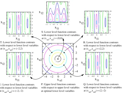
Sub-figure P in Figure 7 shows the contours of the upper level function with respect to the upper level variables assuming the lower level variables to be optimal at eachxu. Sub-figures Q, R, S, T, and U show the behavior of the lower level function at 5 different locations ofxu, which are(2,2),(−2,2),(2,−2),(−2,−2)and(0,0). The problem is once again assumed to have two upper level variables and two lower level variables, such that the dimensions ofxu1,xu2,xl1 andxu2 are all one. The figure shows that there is a different lower level optimization problem at eachxuwhich is required to be solved in order to achieve a feasible solution at the upper level. The contours of the lower level optimization problem differ, based on the location of upper level vector. It can be observed that the rastrigin’s function at the lower level introduces multiple local optima into the problem. The contours of the lower level are further distorted because of the presence of thetan(·)function at the lower level.
In spite of multiple local optima at the lower level, this problem is easier to solve because of the cooperating nature of the functions at the two levels. If a lower level optimization problem is stuck at a local optimum for a particularxu(sayx(0)u ), then it will have a poorer objective function value at the upper level. However, as soon as another lower level optimization problem is solved in the vicinity ofx(0)u , which attains
P: Upper level function contours at optimal lower level variables with respect to upper level variables u2
U: Lower level function contours at (x ,x ) = (−2,−2)u1 u2
T: Lower level function contours at (x ,x ) = (−2,2)u1 u2
S: Lower level function contours at (x ,x ) = (0,0)u1 u2
R: Lower level function contours at (x ,x ) = (2,2)u1 u2
with respect to lower level variables Q: Lower level function contours at (x ,x ) = (2,−2)u1 u2 xu1 x xl1 x l2 xl1 l2 x x x x x l1 l2 l1 l2 l1 l2 x x
with respect to lower level variables
with respect to lower level variables with respect to lower level variables
with respect to lower level variables 30
8 1 4 20 2 10 1 0.1 2 1 1 2 3 10 5 9 15 25 6 9 6 6 4.1 5 9 15 25 6 9 6 6 4.1 5 9 15 25 6 9 6 6 4.1 5 9 15 25 6 9 6 6 4.1
−4 −2 0 2 4
−4 −2 0 2 4 −1.5 −1 −0.5 0 0.5 1 1.5−1.5
−1 −0.5 0 0.5 1 1.5
−1.5 −1 −0.5 0 0.5 1 1.5 1 1.1 1.2 1.3 1.4 1.5
−1.5 −1 −0.5 0 0.5 1 1.5 1 1.1 1.2 1.3 1.4 1.5
−1.5 −1 −0.5 0 0.5 1 1.5 1 1.1 1.2 1.3 1.4 1.5 −1.5−1 −0.5 0 0.5 1 1.5
1 1.1 1.2 1.3 1.4 1.5
Figure 7: Upper and lower level function contours for a four-variable SMD3 test prob-lem.
a global optimum, then it will have a better objective function value at the upper level, and will dominate the previous inaccurate solution. Therefore, a method which is able to handle multi-modality at the lower level at least in few of its lower level optimization runs will be able to successfully solve this problem.
4.4
SMD4
In this test problem there is a conflict between the two levels. The difficulty is in terms of multi-modality at the lower level which once again contains the Rastrigin’s function. The upper level is convex with respect to upper level variables and optimal lower level variables.
F1=P
p i=1(x
i u1)2
F2=−P
q i=1(x
i l1)
2
F3=P
r i=1(x
i u2)2−
Pr
i=1(|x i
u2| −log(1 +xil2)) 2
f1=P
p i=1(x
i u1)2
f2=q+P
q i=1
xil12−cos 2πxil1 f3=Pri=1(|xui2| −log(1 +xil2))2
(21)
The range of variables is as follows, xi
u1∈[−5,10], ∀ i∈ {1,2, . . . , p}
xi
u2∈[−1,1], ∀ i∈ {1,2, . . . , r}
xi
l1∈[−5,10], ∀ i∈ {1,2, . . . , q}
xi
l2∈[0, e], ∀ i∈ {1,2, . . . , r}
P: Upper level function contours at optimal lower level variables with respect to upper level variables u2
U: Lower level function contours at (x ,x ) = (−2,−2)u1 u2
S: Lower level function contours at (x ,x ) = (0,0)u1 u2
R: Lower level function contours at (x ,x ) = (2,2)u1 u2
with respect to lower level variables Q: Lower level function contours at (x ,x ) = (2,−2)u1 u2
xu1 x xl1 x l2 xl1 l2 x x x x x l1 l2 l1 l2 l1 l2 x x
with respect to lower level variables
with respect to lower level variables with respect to lower level variables
with respect to lower level variables T: Lower level function contours at (x ,x ) = (−2,2)u1 u2
30 8 1 4 20 0.1 1 1 1 2 2 2 3 5 4.1 5 5 5 6 6 6 6 6 6 5 4.1 5 5 5 6 6 6 6 6 6 5 4.1 5 5 5 6 6 6 6 6 6 5 4.1 5 5 5 6 6 6 6 6 6 5
−4 −2 0 2 4
−4 −2 0 2 4
−1.5−1−0.5 0 0.5 1 1.5 0 1 2 3 4 5
−1 −0.5 0 0.5 1 3 4 5 6 7 8 9 10
−1 −0.5 0 0.5 1 3 4 5 6 7 8 9 10
−1 −0.5 0 0.5 1 3 4 5 6 7 8 9 10
−1 −0.5 0 0.5 1 3 4 5 6 7 8 9 10
Figure 8: Upper and lower level function contours for a four-variable SMD4 test prob-lem.
Relationship between upper level variables and lower level optimal variables is given as follows,
xil1= 0, ∀ i∈ {1,2, . . . , q} xil2= log−1|xi
u2| −1, ∀ i∈ {1,2, . . . , r}
(23) The values of the variables at the optima arexu = 0andxlis obtained by the rela-tionship given above. Both the upper and lower level functions are equal to zero at the optima.
Figure 8 represents the same information as in Figure 7 for a four-variable bilevel problem. However, this problem involves conflict between the two levels, which make the problem significantly more difficult than the previous test problem. For this test problem if a lower level optimization problem is stuck at a local optimum for a par-ticularxu, then it will end up having a better objective function value at the upper level, than what it will attain at the true global lower level optimum. Therefore, even if another lower lower level optimization problem is successfully solved in the vicinity of xu, the previous inaccurate solution will dominate the new solution at the upper level. This problem can be handled only by those methods which are able to efficiently handle lower level multi-modality without getting stuck in a local basin.
4.5
SMD5
In this test problem, there is a conflict between the two levels. The difficulty introduced is in terms of multi-modality and convergence at the lower level. The lower level problem contains the Rosenbrock’s (banana) function such that the global optimum
lies in a long, narrow, flat parabolic valley. The upper level is convex with respect to upper level variables and optimal lower level variables.
F1=Ppi=1(xiu1)2
F2=−P
q i=1
xil1+1− xil12+ xil1−12
F3=P
r i=1(x
i u2)
2−Pr
i=1(|x i u2| −(x
i l2)
2)2
f1=P
p i=1(x
i u1)
2
f2=P
q i=1
xil+11 − xi l1
2
+ xi
l1−1
2
f3=P
r i=1(|x
i
u2| −(xil2) 2)2
(24)
The range of variables is as follows,
xiu1∈[−5,10], ∀ i∈ {1,2, . . . , p} xiu2∈[−5,10], ∀ i∈ {1,2, . . . , r} xil1∈[−5,10], ∀ i∈ {1,2, . . . , q} xil2∈[−5,10], ∀ i∈ {1,2, . . . , r}
(25)
Relationship between upper level variables and lower level optimal variables is given as follows,
xil1= 1, ∀ i∈ {1,2, . . . , q} xi
l2=
p
|xi
u2|, ∀ i∈ {1,2, . . . , r}
(26) The values of the variables at the optima arexu = 0andxlis obtained by the rela-tionship given above. Both the upper and lower level functions are equal to zero at the optima.
4.6
SMD6
In this test problem, once again there is a conflict between the two levels. This prob-lem is different from previous probprob-lems such that it contains infinitely many global solutions at the lower level, for any given upper level vector. Out of the entire global solution set, there is only a single lower level point which corresponds to the best upper level function value.
F1=P
p i=1(x
i u1)
2 F2=−Pqi=1(xil1)2+
Pq+s
i=q+1(x i l1)2
F3=P
r i=1(x
i u2)2−
Pr
i=1(x i
u2−xil2) 2 f1=Ppi=1(xiu1)2
f2=P
q i=1(x
i l1)
2+Pq+s−1
i=q+1,i=i+2(x i+1
l1 −x
i l1)
2
f3=P
r
i=1(xiu2−xil2)2
(27)
The range of variables is as follows, xi
u1∈[−5,10], ∀ i∈ {1,2, . . . , p}
xi
u2∈[−5,10], ∀ i∈ {1,2, . . . , r}
xi
l1∈[−5,10], ∀ i∈ {1,2, . . . , q+s}
xi
l2∈[−5,10], ∀ i∈ {1,2, . . . , r}
xl1j
xl1i x l1
j
xl1
i
−
(
2
)
2
20 50 10
2 10
20
0
−4 −2
0 2
4 −4
−2 0
2 4
0 20 40 60 80 100
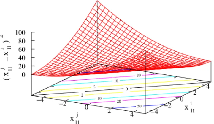
Figure 9: Plot of the term inf2responsible for creating multiple optimum solutions at the lower level. The value of the term is zero at all the points in the valley.
Relationship between upper level variables and lower level optimal variables is given as follows,
xil1= 0, ∀ i∈ {1,2, . . . , q} xil2=xiu2, ∀ i∈ {1,2, . . . , r}
(29) The values of the variables at the optima arexu = 0andxlis obtained by the rela-tionship given above. Both the upper and lower level functions are equal to zero at the optima.
Figure 9 shows the second term ((xi
l1−x
j l1)
2, fors = 2) for functionf
2, and its contours at the lower level. It could be observed from the figure that all the points alongxjl1 = xi
l2have a value 0 for the functionf2. All these points are responsible for introducing multiple global optimal solutions at the lower level for any given upper level variable vector. However, out of all the global optimal solutions at the lower level, the solutionxjl1 =xi
l2 = 0provides the best function value at the upper level for any given upper level variable vector.
4.7
SMD7
In this test problem, we introduce complexities at the upper level, while keeping the lower level optimization task relatively simpler. Most of the previous test problems would be useful to test the ability of algorithms in handling lower level optimization task efficiently. However, this test problem contains multi-modality at the upper level, which demands a global optimization approach at the upper level. The functionF1at the upper level represents a slightly modified Griewank function.
F1= 1 +4001 P p
i=1 x
i u1
2
−Πpi=1cosx√iu1
i
F2=−P
q i=1(x
i l1)
2
F3=P
r i=1(x
i u2)2−
Pr
i=1(x i
u2−logxil2) 2
f1=P
p i=1(x
i u1)3
f2=P
q i=1(x
i l1)
2
f3=P
r i=1(x
i
u2−logxil2) 2
(30)
The range of variables is as follows,
xiu1∈[−5,10], ∀ i∈ {1,2, . . . , p} xiu2∈[−5,1], ∀ i∈ {1,2, . . . , r} xil1∈[−5,10], ∀ i∈ {1,2, . . . , q} xi
l2∈(0, e], ∀ i∈ {1,2, . . . , r}
(31)
Relationship between upper level variables and lower level optimal variables is given as follows,
xil1= 0, ∀ i∈ {1,2, . . . , q} xi
l2= log
−1xi
u2, ∀ i∈ {1,2, . . . , r}
(32) The values of the variables at the optima arexu = 0andxlis obtained by the rela-tionship given above. Both the upper and lower level functions are equal to zero at the optima.
4.8
SMD8
This test problem once again tests the ability of the algorithms in handling multi-modality at the upper level, and handling a complex lower level problem at the same time. There is also a conflict between the upper level and lower level optimization tasks. The lower level objective contains the Rosenbrock’s (banana) function, and the upper level objective contains the multi-modal Ackley’s function.
F1= 20 +e−20exp
−0.2q1
p
Pp
i=1(xiu1)2
−exp1pPp
i=1cos 2πxiu1
F2=−Pqi=1
xil+11 − xi l1
2
+ xi
l1−1
2
F3=P
r i=1(x
i u2)2−
Pr
i=1(x i
u2−(xil2) 3)2
f1=P
p i=1|x
i u1|
f2=P
q i=1
xil+11 − xi l1
2
+ xi
l1−1
2
f3=Pri=1(xiu2−(xil2)3)2
(33) The range of variables is as follows,
xi
u1∈[−5,10], ∀ i∈ {1,2, . . . , p}
xi
u2∈[−5,10], ∀ i∈ {1,2, . . . , r}
xi
l1∈[−5,10], ∀ i∈ {1,2, . . . , q}
xi
l2∈[−5,10], ∀ i∈ {1,2, . . . , r}
Relationship between upper level variables and lower level optimal variables is given as follows,
xi
l1= 0, ∀ i∈ {1,2, . . . , q}
xil2= (xiu2)
1
3, ∀ i∈ {1,2, . . . , r} (35)
The values of the variables at the optima arexu = 0andxlis obtained by the rela-tionship given above. Both the upper and lower level functions are equal to zero at the optima.
4.9
SMD9
In this test problem, we introduce constraints at both upper and lower levels. Con-straints are defined such that they causes convergence difficulties at both levels inde-pendently. One constraint is introduced at each level, such that the upper level con-straint is a function of the upper level variables, and the lower level concon-straint is a function of the lower level variables. The constraints divide the search space into an-nular regions, and causes convergence difficulties without altering the global optimum. The constraint at the upper as well as the lower level is however, inactive at the opti-mum. The two levels are once again conflicting in nature, such that, an inaccurate lower level optimum may lead to upper level function value better than the true optimum for the bilevel problem.
F1=Ppi=1(xiu1)2 F2=−Pqi=1(xil1)2
F3=P
r
i=1(xiu2)2−
Pr
i=1(xiu2−log(1 +xil2))2
f1=P
p
i=1(xiu1)2
f2=P
q i=1(x
i l1)
2
f3=P
r i=1(x
i
u2−log(1 +xil2)) 2
(36)
The upper and lower level constraints are as follows: Upper level constraint
G1:
Pp
i=1(x
i u1)2+
Pr
i=1(x
i u2)2
a −
jPp i=1(x
i u1)2+
Pr
i=1(x
i u2)2
a +
0.5 b
k
≥0
Lower level constraint g1:
Pp
i=1(x
i l1)2+
Pr
i=1(x
i l2)2
a −
jPp i=1(x
i l1)2+
Pr
i=1(x
i l2)2
a +
0.5 b
k
≥0
Wherea= 1andb= 1.
(37)
The range of variables is as follows, xi
u1∈[−5,10], ∀ i∈ {1,2, . . . , p}
xi
u2∈[−5,1], ∀ i∈ {1,2, . . . , r}
xil1∈[−5,10], ∀ i∈ {1,2, . . . , q}
xil2∈(−1,−1 +e], ∀ i∈ {1,2, . . . , r}
(38)
Relationship between upper level variables (feasible with respect to upper level con-straints) and lower level optimal variables is given as follows,
xi
l1= 0, ∀ i∈ {1,2, . . . , q}
xi
l2= log
−1 xi
u2−1, ∀ i∈ {1,2, . . . , r}
x x
u2
u1 −2
0 2 4
−4 −2 0 4
Feasible Region
Infeasible Region
−4
2
Figure 10: Feasible and infeasible regions in case of a two-variable constraint function.
Figure 10 shows the restricted search space for the upper level optimization task when it is a function of two upper level variables, i.e. p= 1andr = 1. The search space looks similar at the lower level whenq= 1andr= 1. For higher number of variables, the annular rings transform into spherical shells. The values of the variables at the optima arexu= 0andxl = 0. Both the upper and lower level functions are equal to zero at the optima.
4.10
SMD10
In this test problem, we introduce constraints at the upper as well as the lower level such that they are scalable. As the number of variables are varied at the upper and the lower levels, the number of constraints also vary. This is different from the previous problem such that all the constraints are active at the optimum. However, in this function once again we have the upper level constraints as functions of the upper level variables, and the lower level constraints as functions of the lower level variables.
F1=P
p i=1(x
i
u1−2)
2
F2=P
q i=1(x
i l1)
2
F3=P
r i=1(x
i
u2−2)2−
Pr
i=1(x i
u2−tanxil2) 2
f1=P
p i=1(x
i u1)2
f2=P
q i=1(x
i l1−2)
2
f3=P
r i=1(x
i
u2−tanxil2) 2
The upper and lower level constraints are as follows: Upper level constraints
Gj :x
j
u1−
Pp
i=1,i6=j(x i u1)3−
Pr
i=1(x i
u2)3≥0, ∀j∈ {1,2, . . . , p} Gp+j :xju2−
Pr
i=1,i6=j(x i u2)3−
Pp
i=1(x i
u1)3≥0, ∀j ∈ {1,2, . . . , r} Lower level constraints
gj:xjl1−Pq
i=1,i6=j(x i l1)
3≥0, ∀j∈ {1,2, . . . , q}
(41)
The range of variables is as follows, xi
u1∈[−5,10], ∀ i∈ {1,2, . . . , p}
xi
u2∈[−5,10], ∀ i∈ {1,2, . . . , r}
xi
l1∈[−5,10], ∀ i∈ {1,2, . . . , q}
xil2∈(−2π,π2), ∀ i∈ {1,2, . . . , r}
(42)
Relationship between upper level variables (feasible with respect to upper level con-straints) and lower level optimal variables is given as follows,
xi
l1=
1
√
q−1, ∀ i∈ {1,2, . . . , q} xil2= tan−1xiu2, ∀ i∈ {1,2, . . . , r}
(43)
The values of the variables at the optima arexu= √ 1
p+r−1, andxlis obtained by the relationship given above.
Figure 11 shows the feasible region of the search space for the upper level opti-mization task, when the upper level objective it is a function of two upper variables,
i.e. p = 1, r = 1. The shaded part in the figure shows the feasible region, and
the dotted lines show the contours of the upper level objective function. For such a two variable upper level objective function, the optima lies at one of the intersections ((xu1,xu2) = (1,1)) of the constraints shown in the figure.
4.11
SMD11
In this test problem, we introduce constraints which are functions of upper as well as lower variables at both levels. The constraints at the upper level are scalable, but there is just a single constraint at the lower level. The constraint at the lower level introduces multiple global optimal solutions at the lower level for any given upper level vector. At the optimum of the bilevel problem, the lower level constraint is active as well as the upper level constraints are active. The upper level constraints eliminate a large part of the global optimal solutions from the lower level.
F1=Ppi=1(xiu1)2 F2=−Pqi=1(xil1)2 F3=Pri=1(xiu2)2−
Pr i=1(x
i
u2−logxil2)2
f1=P
p
i=1(xiu1)2
f2=P
q i=1(x
i l1)
2
f3=P
r i=1(x
i
u2−logx
i l2)
2
x x
u1 u2
25
16 9
1
2 0.25
4
Region Feasible
x − (x ) >= 0
3
x − (x ) >= 0u1 u2 u2
3 u1
−1 1 2 3 3
2
1
0
−1
−2
−3
−3 −2 0
Figure 11: Feasible and infeasible regions in case of a two-variable constraint function.
The upper and lower level constraints are as follows: Upper level constraints
Gj:xju2≥ √1
r+ logx
j
l2, ∀j∈ {1,2, . . . , r} Lower level constraint
g1:P
r i=1(x
i
u2−logxil2)
2≥1
(45)
The range of variables is as follows, xi
u1∈[−5,10], ∀ i∈ {1,2, . . . , p}
xi
u2∈[−1,1], ∀ i∈ {1,2, . . . , r}
xi
l1∈[−5,10], ∀ i∈ {1,2, . . . , q}
xi l2∈[
1
e, e], ∀ i∈ {1,2, . . . , r}
(46)
Relationship between upper level variables and lower level optimal variables is given as follows,
xi
l1= 0, ∀ i∈ {1,2, . . . , q}
xl2:Pri=1(xiu2−logxil2)2= 1
(47) The values of the variables at the optima arexu1 = 0,xu2 = 0,xl1 = 0, andxl2 = log−1−√1
r. The upper level function value is−1and the lower level function value is +1at the optima.
Figure 12 shows the constraints at the upper as well as the lower level whenr= 2. In this example, there is one constraint at the lower level and two constraints at the upper level. All the solutions on the lower level constraint represent optimal solutions to the lower levelf3. Whenxl1 = 0, such that the function f2 is also optimal, the solutions on the constraint are optimal solutions to the lower level problem for a given xu. It can be observed that the two constraints at the upper level eliminate all the lower level optimal solutions except one. The figure shows feasible region with respect to
x
xl2 l2
(x ,x ) = (0,0)u2 u2
1 2
2 1
LL Optimal LL Constraint Feasible Region LL Constraint
UL Constraint Feasible Region
UL Constraints
0 0.5 1 1.5 2 2.5 3
0 0.5 1 1.5 2 2.5 3 p
Figure 12: Feasible and infeasible regions of SMD11 for a particular upper level vector.
upper level constraints for the upper level problem. However, only pointprepresents a feasible solution for the upper level problem for a givenxu, as it is the lower level optimal solution lying in the upper level constraint feasible region. This problem differs from SDM6, which also contained multiple global solutions at the lower level, in two ways. Firstly, multiple global solutions at the lower level are introduced by lower level constraints in this problem, whereas in the previous problem, it was the lower level objective function which was entirely responsible for introducing multiple global solutions. Secondly, out of the multiple global solutions from the lower level, a single solution is selected based on upper level constraints, whereas in the previous problem all the lower level global solutions were feasible, but one of those solutions had the best upper level objective value.
4.12
SMD12
This test problem is a combination of the previous two test problems, and involves a number of difficulties. The test problem has scalable constraints at both levels, and the constraints are a function of both upper as well as lower level variables. At the same time, any lower level optimization problem for a given set of upper level variables has multiple global optima. All the lower level constraints are active at the bilevel optimum.
F1=P
p i=1(x
i
u1−2)
2
F2=P
q i=1(x
i l1)
2
F3=P
r i=1(x
i
u2−2)2+
Pr
i=1tan|x
i l2| −
Pr
i=1(x i
u2−tanxil2) 2
f1=P
p i=1(x
i u1)2
f2=P
q i=1(x
i l1−2)
2
f3=P
r i=1(x
i
u2−tanxil2) 2
The upper and lower level constraints are as follows: Upper level constraints
xiu2−tanxil2≥0, ∀i∈ {1,2, . . . , r} xju1−Pp
i=1,i6=j(x i u1)3−
Pr
i=1(x i
u2)3≥0, ∀j∈ {1,2, . . . , p} xju2−Pr
i=1,i6=j(x i u2)3−
Pp
i=1(x i
u1)3≥0, ∀j∈ {1,2, . . . , r} Lower level constraints
Pr
i=1(x i
u2−tanxil2)
2≥1
xjl1−Pp
i=1,i6=j(x i
l1)3, ∀j∈ {1,2, . . . , q}
(49)
The range of variables is as follows,
xiu1∈[−5,10], ∀ i∈ {1,2, . . . , p} xi
u2∈[−14.10,14.10], ∀ i∈ {1,2, . . . , r}
xi
l1∈[−5,10], ∀ i∈ {1,2, . . . , q}
xi
l2∈(−1.5,1.5), ∀ i∈ {1,2, . . . , r}
(50)
Relationship between upper level variables and lower level optimal variables is given as follows,
xi
l1=
1
√
q−1, ∀ i∈ {1,2, . . . , q}
xl2:P
r i=1(x
i
u2−tanx
i l2)
2= 1 (51)
The values of the variables at the optima arexu1 = √p+1r−1,xu2 = √p+1r−1,xl1 = √
q−1, andxl2= tan−1(√p+1r−1−√1r).
4.13
Summary
The properties of the SMD test problems are summarized in Table 3. In the table,
N = NoandY = Yes. It can be observed that the 12 test problems are a good mix
of various difficulties, which we discussed in the prior sections. We have tried to put the problems in an increasing order of difficulty. The last test problem can be observed to contain most of the difficulties except multi-modalities. This table will be helpful in testing algorithms for bilevel optimization. For example, if a new algorithm is able to solve SMD1 but not SMD2, one readily concludes that the algorithm is unable to handle a conflict. Similarly, if the algorithm is able to solve SMD1 and SMD2 but not SMD3 and SMD4, one would infer that the algorithm is unable to handle lower level multi-modality. Such information will be useful for an algorithm developer, as it helps him to identify the specific weaknesses in his approach, which he needs to improve on.
5
Baseline Solution Methodology
In this section, we describe the solution methodology used to solve the constructed test problems. The suggested procedure is a nested bilevel evolutionary algorithm, and requires that a lower level optimization task be solved for every new set of upper level variables produced using the genetic operators. The method relies on a steady state single objective real coded genetic algorithm to solve the problems at both levels.
Table 3: Properties of SMD test problems.
SMD Conflict
Constrained Multi-‐modality Constrained Multi-‐modality Multiple Variables Constraints Variables Constraints Global Solutions
1 N Y -‐ N N Y -‐ N N N
2 N Y -‐ N N Y -‐ N N Y
3 N Y -‐ N N Y -‐ Y N N
4 N Y -‐ N N Y -‐ Y N Y
5 N Y -‐ N N Y -‐ Y N Y
6 N Y -‐ N N Y -‐ N Y Y
7 N Y -‐ Y N Y -‐ N N Y
8 N Y -‐ Y N Y -‐ Y N Y
9 Y Y N N Y Y N N N Y
10 Y Y Y N Y Y Y N N Y
11 Y Y Y N Y Y N N Y Y
12 Y Y Y N Y Y Y N Y Y
Upper Level Lower Level
Scalability Scalability
We have implemented a modified version of the procedures [16, 15], which is used to handle the bilevel test problems. The proposed method is based on a single objective Parent Centric Crossover (PCX) [8]. A step-by-step procedure for the algorithm is described as follows:
5.1
Upper Level Optimization Procedure
Step 1: Initialization Scheme. Initialize a random population (Np) of upper level
variables. For each upper level population member execute a lower level optimization procedure to determine the corresponding optimal lower level variables. Assign upper level fitness based on the upper level function value and constraints.
Step 2: Selection of upper level parents.Choose2µpopulation members from the
previous population and conduct a tournament selection to determineµparents.
Step 3: Evolution at the upper level. Perform a PCX based crossover [8] (Refer
Sub-section 5.4) and a polynomial mutation to createλoffsprings. This provides the upper level variables for each offspring.
Step 4: Lower level optimization.Solve the lower level optimization problem
(Re-fer Sub-section 5.2) for each offspring. This provides the lower level variables for each offspring.
Step 5: Evaluate offsprings. Combine the upper level variables with the
corre-sponding optimal lower level variables for each offspring. Evaluate all the offsprings based on upper level function value and constraints.
Step 6: Population update.Chooserrandom members from the parent population
and pool them with theλoffsprings. The bestrmembers from the pool replace the chosenrmembers from the population.
Step 7: Termination check.Proceed to the next generation (Step 2) if the