Depth from Defocus vs. Stereo: How Different Really Are They?

Depth from Defocus vs. Stereo: How Different Really Are They?

YOAV Y. SCHECHNER

Department of Electrical Engineering, Technion—Israel Institute of Technology, Haifa 32000, Israel

yoavs@tx.technion.ac.il

NAHUM KIRYATI

Department of Electrical Engineering-Systems, Faculty of Engineering, Tel-Aviv University, Ramat Aviv 69978, Israel

nk@eng.tau.ac.il

Abstract. Depth from Focus (DFF) and Depth from Defocus (DFD) methods are theoretically unified with the geometric triangulation principle. Fundamentally, the depth sensitivities of DFF and DFD are not different than those of stereo (or motion) based systems having the same physical dimensions. Contrary to common belief, DFD does not inherently avoid the matching (correspondence) problem. Basically, DFD and DFF do not avoid the occlusion problem any more than triangulation techniques, but they are more stable in the presence of such disruptions. The fundamental advantage of DFF and DFD methods is the two-dimensionality of the aperture, allowing more robust estimation. We analyze the effect of noise in different spatial frequencies, and derive the optimal changes of the focus settings in DFD. These results elucidate the limitations of methods based on depth of field and provide a foundation for fair performance comparison between DFF/DFD and shape from stereo (or motion) algorithms.

Keywords: Defocus, depth from focus, depth of field, depth sensing, range imaging, shape from X, stereo, triangulation

1. Introduction

In recent years range imaging based on the lim-ited depth of field (DOF) of lenses has been gaining popularity. Methods based on this principle are nor-mally considered to be a separate class, distinguished from triangulation techniques such as depth from stereo, vergence or motion (Besl, 1988; Engelhardt and Hausler, 1988; Jarvis, 1983; Krotkov and Bajcsy, 1993; Marapane and Trivedi, 1993; Scherock, 1991; Stewart and Nair, 1989; Subbarao et al., 1997). Cooperation between depth from focus, stereo and vergence proce-dures has been studied in Abbott and Ahuja (1988, 1993), Dias et al. (1992), Kristensen et al. (1993), Krotkov and Bajcsy (1993), Stewart and Nair (1989), and Subbarao et al. (1997). Cooperation of depth from defocus with stereo was considered in Darwish (1994), Klarquist et al. (1995), and Subbarao et al. (1997).

Successful application of computer vision algo-rithms requires sound performance evaluation and comparison of the various approaches available. The comparison of range sensing systems that rely on dif-ferent principles of operation and have a wide range of physical parameters is not easy (Besl, 1988; Jarvis, 1983). In particular, in such cases it is difficult to distin-guish between limitations of algorithms to those arising from fundamental physical bounds.

The following observations and statements are com-mon in the literature:

1. The resolution and sensitivity of Depth from De-focus (DFD) methods are limited in compari-son to triangulation based techniques (Besl, 1988; Hwang et al., 1989; Pentland, 1987; Pentland et al., 1989, 1994; Rajagopalan and Chaudhuri, 1997; Stewart and Nair, 1989; Subbarao, 1988; Subbarao and Surya, 1994; Subbarao and Wei,

1992; Subbarao et al., 1997; Surya and Subbarao, 1993).

2. Unlike triangulation methods, DFD avoids the missing-parts (occlusion) problem (Bove, 1989, 1993; Ens and Lawrence, 1993; Nayar et al., 1995; Pentland et al., 1994; Saadat and Fahimi, 1995; Scherock, 1991; Subbarao and Liu, 1996; Subbarao and Surya, 1994; Subbarao and Wei, 1992; Subbarao et al., 1997; Surya and Subbarao, 1993; Watanabe and Nayar, 1996).

3. Unlike triangulation methods, DFD avoids match-ing (correspondence) ambiguity problems (Bove, 1989, 1993; Darwish, 1994; Ens and Lawrence, 1993; Hwang et al., 1889; Nayar et al., 1995; Pentland, 1987; Pentland et al., 1989, 1994; Rajagopalan and Chaudhuri, 1995a; Saadat and Fahimi, 1995; Scherock, 1991; Simoncelli and Farid, 1996; Subbarao and Liu, 1996; Subbarao and Surya, 1994; Subbarao and Wei, 1992; Subbarao et al., 1997; Surya and Subbarao, 1993; Swain et al., 1994; Watanabe and Nayar, 1996; Xiong and Shafer, 1993).

4. DFD is reliable (Nayar et al., 1995; Pentland, 1987; Pentland et al., 1989; Subbarao and Wei, 1992).

Similar statements were made with regard to Depth from Focus (DFF) (Abbott and Ahuja, 1993; Darrell and Wohn, 1988; Dias et al., 1992; Engelhardt and Hausler, 1988; Krotkov and Bajcsy, 1993; Marapane and Trivedi, 1993; Subbarao and Liu, 1996). There have been several attempts to explain these observa-tions. For example, the limited sensitivity of DFD was associated with suboptimal selection of param-eters (Rajagopalan and Chaudhuri, 1997), leading to interest in optimizing the changes in imaging system parameters. A major step towards understanding the relations between triangulation and DOF has been re-cently taken in Adelson and Wang (1992), Farid (1997), and Farid and Simoncelli (1998). A large aperture lens was utilized to build a “monocular stereo” system, with sensitivity that has the same functional dependence on parameters as in a stereo system (without vergence).

We show that the difference between methods that rely on the limited depth of field of the optical system (DFD and DFF) and “classic” triangulation techniques (stereo, vergence, motion) is mainly due to technical reasons, and is hardly a fundamental one. In fact, DFD and DFF can be regarded as ways to achieve triangu-lation. We study the fundamental characteristics of the above mentioned methods and the differences between

them in a formal and quantitative manner. The first statement above claims superiority of stereo over DFD with regard to sensitivity. However, the origins of this observation are primarily in the physical size differ-ence between common implementations of focus and triangulation based systems, not in the fundamentals. Generally, this statement does not hold.

As to the second and third statements (that un-like stereo, the occlusion and matching problems are avoided in DFD), they again follow mainly from phys-ical size differences in the common implementations. As they are expressed, these two statements do not hold. Actually, we note a fundamental matching problem in DFD, analogous to the problem in stereo. There are, however, some differences between DFD, stereo, and DFF with respect to matching ambiguity and occlusion that can be expressed quantitatively.

In contrast, the fourth observation (reliability of DFD) has a solid foundation. DFF and DFD rely on more data than common discrete triangulation meth-ods, and are thus potentially more reliable. Note that an approach and algorithm similar to DFD can also be ap-plied in Depth from Motion Blur (smear) (Fox, 1988), leading to improved robustness. Still, unlike motion smear which is one dimensional (1D), DFF and DFD rely on two dimensional (2D) blur and thus have an important advantage.

In order to study the influence of noise on the various ranging methods considered in this paper, we analyze its effect in each spatial frequency of which the image is composed. We show that some frequencies are more useful for range estimation, while others do not make a significant or reliable contribution. Our analysis leads to a new property of depth of field: it is the optimal interval between focus-settings in depth-from-defocus for robustness to perturbations. We also show that in DFD, if the step used is larger by a factor of 2 or higher, the estimation process may be very unstable. We thus obtain the limits on the interval between focus settings that ensures stable operation of DFD. Some prelimi-nary results were presented in Schechner and Kiryati (1998, 1999).

2. Sensitivity 2.1. DFD

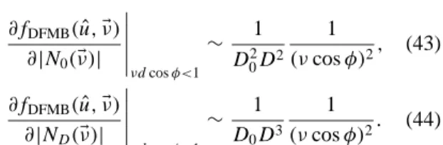
Consider the imaging system sketched in Fig. 1. The sensor at distancev˜behind the lens can image in-focus a point at distanceu in front of the lens. An object point˜

Figure 1. The imaging system with an aperture D is tuned to view in focus object points at distanceu. The image of an˜

object point at distance u is a blur circle of radius r in the sensor plane.

at distance u is defocused, and its image is a blur-circle of radius r in the sensor plane.

In this system the blur radius is (Scherock, 1991)

r = D

2

|uF− ˜vu+Fv˜|

Fu (1)

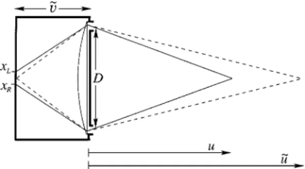
where F is the focal length and D is the aperture of the lens. For simplicity we adopt the common assumption that the system is invariant to transversal shift. This is approximately true for paraxial systems, where the angles between light rays and the optical axis are small. Suppose now that the entire lens is blocked, except for two pinholes on its perimeter, on opposite ends of some diameter (Adelson and Wang, 1992; Hiura et al., 1998), as shown in Fig. 2. Only two rays pass the lens. The geometrical point spread function (PSF) thus

con-Figure 2. An imaging system similar to that of Fig. 1, with its lens blocked except for two pinholes on its perimeter, on opposite ends of some diameter. The image of an out-of-focus object point is two points, with disparity equal to the diameter of the blur circle that would have appeared had the blocking been removed.

Figure 3. A stereo system with a baseline D equal to the lens diameter in Fig. 1. The distancev˜ from the entrance pupil to the sensor is also the same. The vergence eliminates the disparity for the object point at distanceu. The result-˜

ing disparity caused by the object point at u is equal to the diameter of the blur kernel formed by the system of Fig. 1.

sists of only two points, xL and xR. The distance

be-tween the points is

|xR−xL| =2r. (2)

The fact that the image of each object point consists of two points, separated by a distance that depends on the depth of the object, gives rise to the analogy to stereo. Note that for an object point at a distanceu, the˜

image points coincide, i.e. have no disparity. To accom-modate this in the analogy, we incorporate vergence into the stereo system. Now, consider the stereo & ver-gence system shown in Fig. 3 that consists of two pin-hole cameras. It has the same physical dimensions as the system shown in Fig. 1, i.e., the baseline between the pinholes is equal to the width of the large aper-ture lens, and the sensors are at the same distancev˜ behind the pinholes. The image of an object point at

u is again two points, now one on each sensor. Since

the angles are small (e.g., D¿u) the disparity can be

well approximated by

d= ˆxR− ˆxL=DuF− ˜vu+Fv˜

Fu =Df(u). (3)

Comparing this result to Eqs. (1) and (2) we see that | ˆxR− ˆxL| = |xR−xL| =2r. (4)

The same result is also obtained for u >u. Thus, for˜ a triangulation system with the same physical dimen-sions as a DFD system, the disparity is equal to the size of the blur kernel. An alternative interpretation is

to consider the stereo baseline as a synthetic aperture of an imaging system. A proportion between the disparity and blur-diameter in a system as Fig. 2 (with the holes on the diameter having a finite support) was noticed in Adelson and Wang (1992).

The sensitivity (and resolution) of the triangulation systems are equivalent to those of DFD systems and are related to the disparity/PSF-support size (Eq. (4)): Depth deviation from focus is sensed if this value is larger than the pixel period1 _{1x (See Refs. (Abbott}

and Ahuja, 1993; Engelhardt and Hausler, 1988) and Subsection 5.5). The conclusion is that methods that

rely on the depth of field are not inherently less sen-sitive than stereo or motion. In particular the rate of

decrease of the resolution with object distance is fun-damentally the same. In practice, however, the typi-cal lens apertures used (Adelson and Wang, 1992) are merely in the order of∼1 cm while stereo baselines are usually one or two orders of magnitude larger, leading to a proportional increase of the sensitivity.

It is interesting to note that the common limits on lens apertures can be broken by the use of holographic optical elements (HOE). Holographic “lenses” are very thin, yet allow the deviation of rays by large angles. The design of such elements for imaging purposes is non-trivial, but HOE are actually in use in wide-angle head-up and helmet displays for aircraft (Amitai et al., 1989).

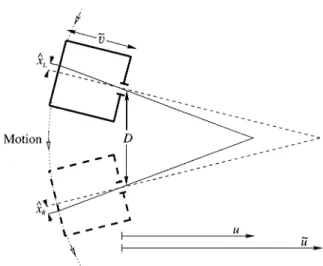
Consider depth from motion, that can be regarded as a “classic” triangulation approach. We shall see that it provides an effect analogous to 1D defocus blur. If discrete images are taken, the baseline between the ini-tial and final frames dictates the depth resolution. Most DFD and motion approaches differ in the algorithms used: In DFD the support of the blur kernel is calculated by comparison to a small-aperture (reference) image, while motion based analysis relies on matching. How-ever, the principle of operation of Depth from Motion

Blur (DFMB) (Fox, 1988), is similar to DFD: A

fast-shutter photograph is compared to an image blurred by the camera motion (slow shutter), to estimate the motion extent (Chen et al., 1996), from which depth is extracted (Fig. 4).

The analogy between DFD and DFMB can be en-hanced by demonstrating the equivalent to a focused point in motion blur. Consider the system shown in

Figure 4. While the shutter is open, the camera moves along an arc, pointing to the arc axis atu. This point is sharply˜

imaged while closer or farther points are motion blurred, in a manner analogous to defocus.

Fig. 4. The camera moves along an arc of radius u,˜

with its optical axis pointing towards the center of the circle. While the scene is generally motion blurred, a point at a distanceu remains unblurred! The analo-˜

gous DFD system is constructed by removing part of the blocking shown in Fig. 2, exposing a thin line on the lens, between the former pinholes (thus the system can still be analyzed as having a single transversal dimen-sion). Thus, the analysis of the spread is not based only on the two marginal points, but on a 1D continuum of points.

2.2. DFF

In DFF, depth is estimated by searching for the state of the imaging system for which the object is in-focus. Referring to Fig. 1, this may be achieved by chang-ing eitherv˜(the lens to sensor distance), F (the focal length) or u (the object distance), or any combination of them. Images are taken for each incremental change of these parameters. The state of the set-up for which the best-focused image was taken indicates the depth by the relation

1 ˜

u =

1

F −

1 ˜

v. (5)

The process of changing the camera parameters to achieve a focused state is analogous to changing the

convergence angle between two cameras in a typi-cal triangulation system. This qualitative analogy has been stated before (Abbott and Ahuja, 1988; Pentland, 1987; Pentland et al., 1989). This can be seen clearly in Figs. 1–3. For example, focusing the system of Fig. 1 by axial movement towards/away from the object point changes u, to have u → ˜u, until the blur-radius is

zero (or undetectable) has the same effect as moving the stereo system of Fig. 3 in that direction. Alterna-tively, focusing by changing the focal length F does not induce magnification, but shifts v so that v→ ˜v by changing the refraction angles of the light-rays in Figs.1 and 2. This has the same effect as changing the convergence angle in Fig. 3. Focusing by axially mov-ing the sensor changesv˜so thatv˜ →v. This changes the magnification as well as the angles of the light-rays which hit the sensor at focus. This has the same ef-fect as changing bothv˜ and the convergence angle in Fig. 3. We note that magnification corrections (Darrell and Wohn, 1988; Nair and Stewart, 1992; Subbarao, 1988), which are usually insignificant (Stewart and Nair, 1989; Subbarao and Wei, 1992), enable focusing when the settings change is accompanied with magni-fication change.

The sensitivity to changes in parameters in DFF is related to the smallest detectable blur-diameter, while the sensitivity in stereo & vergence is related to the smallest detectable disparity. Both the disparity and the blur-diameter are sensed if they are larger than the pixel period. Since for the same system dimensions the blur-diameter and the disparity are the same, the sensitivity of DFF is similar to that of depth from convergence.

In Stewart and Nair (1989) the disparity in a stereo image pair was found empirically to be approximately linearly related to the focused state setting of a DFF system. We can now explain this result analytically. Suppose the system is initially focused at infinity. In order to focus on the object at u, the sensor has to be moved by

1v˜=v−F, (6)

which according to Eq. (5) is 1v˜= Fv

u . (7)

The sensor positionv˜, or its distance1v˜from the focal point, indicate the focus setting. The stereo baseline is

Dstereo. In the system of Stewart and Nair (1989), the

stereo system was fixated at infinity thus the disparity

was

d =Dstereo·v˜

u =Dstereo· v

u, (8)

where in the right hand side of Eq. (8) we assumed that the disparity was measured at the state for which the object was focused, in that cooperative system. Com-bining Eqs. (7) and (8) we get

d= Dstereo

F 1v˜ (9)

which is a linear relation between the focus setting and the disparity. If focusing is achieved differently (e.g. moving the lens but keeping the sensor position fixed), there are higher order terms in the relation be-tween focus-setting and disparity, but in practice they are negligible compared to the linear dependence.

3. Occlusion 3.1. DFD

The observation that monocular methods are not prone to the missing parts (occlusion) problem is mostly a consequence of the small “baseline” associated with the lens. The small angles involved reduce the num-ber of points that will be visible to a part of the lens while being occluded at another part (vignetting caused by the scene). However, such incidents may occur (Adelson and Wang, 1992; Asada et al., 1998; Farid, 1997; Marshall et al., 1996).

Note that the same applies to stereo (Simoncelli and Farid, 1996) (or motion) with the same baseline! Al-though mechanical constraints usually complicate the construction of stereo systems with a small baseline, such systems can be made. An example is the “monoc-ular stereo” system presented in Farid and Simoncelli (1998), whose principle of operation is similar to that shown in Fig. 2. Another possibility is to position a beam-splitter in front of the triangulation system. There is, of course, no “free lunch”: the avoidance of the oc-clusion problem (and also the correspondence problem as will be discussed in Section 4) by decreasing the baseline leads to a reduction in sensitivity (Pentland et al., 1994).

The main differences between DFD and common triangulation methods arise when we consider the 2D nature of the image. It turns out that for the same system dimensions, the chance of occurrence of the

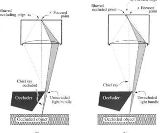
Figure 5. The stereo PSF consists of two distinct impulse func-tions. The line segment that defines the disparity between them is the support of the motion blur kernel, and the diameter of the defocus blur kernel for the same system dimensions. An occluding object is in-focus (and in perfect convergence in the stereo case) in this dia-gram, hence has sharp boundaries. In (a) the object is occluding only a DFD setup but not the stereo/motion setups. In (b) occlusion makes stereo matching impossible, and an error occurs in DFMB and DFD. In DFD, the diameter parallel to the occluding edge makes error-free recovery possible.

occlusion phenomenon is higher for DFD than for stereo (Fig. 5(a)). This is due to the fact that the

de-focus point-spread is much larger than for stereo. That is, there may be many situations in which occlusion oc-curs for the DFD system, and not for the stereo system. Nevertheless, there is a difference in the conse-quences of occlusion. In stereo, the fact that one of the rays is blocked makes matching and depth estima-tion impossible (Fig. 5(b)). In contrast, DFD relies on a continuum of rays, thus allowing estimation, although with an error. If the occluded part is small compared to the support of the blur-kernel, and its depth is close to that of the occluding object, the error will be small. Depth from motion blur, acquired as described in Fig. 4 (or even a discrete sequence of images acquired as the camera is in motion) will have a similar stable behavior (Fig. 5(b)).

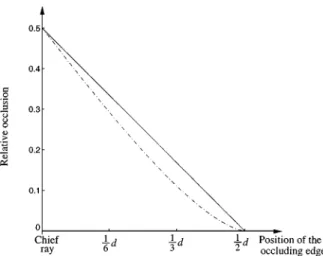
Consider small occlusions, covering less than half the blur PSF. In these cases the chief ray (the light ray that would have passed through a pinhole camera and marks the center of the PSF) is not occluded.2_As

seen in Fig. 6 the relative error in the support of the defocus blur is smaller than that of motion blur. This is an advantage of DFD over DFMB. Moreover, from Fig. 5 one can notice that with DFD it is also possible (although not by the current algorithms known to us) to fully recover the true blur diameter using a line in the PSF that is parallel to the occluding edge.

Evidence of problems near occlusion boundaries in a “monocular stereo” system is reported in Adelson and Wang (1992). These problems occur since some

Figure 6. The occluding edge of Fig. 5b is at a certain distance to the right of the chief ray. For small occlusions the chief ray is visible and the relative part of the PSF that is occluded is smaller for DFD [dashed line] than for motion [solid line].

points in the scene were occluded to certain parts of the lens aperture. Had that system been used for DFF/DFD, similar occlusions would have taken place. Ref. (Adelson and Wang, 1992) reported that the oc-clusion effect is small. This is due to the small baseline associated with that system. Experimental evidence of the phenomenon is also reported in Asada et al. (1998).

To conclude, DFD does not avoid the occlusion prob-lem anymore than stereo/motion methods (on the con-trary). It is, however more stable to such disruptions. In principle, with DFD it is possible to fully recover the depth as long as the occlusion is small.

3.2. DFF

From the discussion in Subsection 3.1, it follows that occlusion is present also in DFF. In a stereo system with a baseline that is as small as the aperture of typ-ical DFF systems, the occlusion phenomenon would be much less noticeable than in a stereo system with a large baseline. Moreover, as described in Fig. 5(a), for systems of the same physical dimensions the chance of

occlusion is higher in DFF than in stereo due to the 2D

nature of the PSF.

The imaging of occluded objects by finite aperture lenses was analyzed in Marshall et al. (1996). Since the occluding object is out of focus, it is blurred. However, this object causes vignetting to the objects behind it. Thus, the occluded object fades into the occluder. If

the occluded object is left of the occluding edge (in the image space), the image obtained using an aperture D is

gD = Occluded·(1−hD∗Step(x0))

+Occluder∗hD, (10)

where Step(x0) is the step-function at the occluding

edge position x0. In Eq. (10) the blur kernel hD of

the occluding object has a radius r while the occluded object (for which we seek focus) is assumed to be focused.

Inspecting Figs. 7 and 8, there are four classes of image points:

1. x <x0−r . The point is not occluded. Depth at the

point is unambiguous.

2. x0−r ≤ x < x0. The point is slightly occluded

(See Fig. 7(a)). The chief ray from this object point reaches the lens. The point may appear focused but the disturbance of the blurred occluder may shift the estimation of the plane of best focus in DFF. In a stereo & vergence system of the same physi-cal dimensions, each of the two pinholes will see a different object, either the occluder or the occluded one. Thus fixation is ill posed (no solution). 3. x0 ≤ x ≤ x0+r . The point is severely occluded.

The chief ray from this object point does not reach

Figure 7. (a) If the chief ray is not occluded but resides within the blurred image of the occluding edge (slight occlusion) focusing is possible but may be erroneous. (b) For the same system dimensions matching the occluded object point in the stereo/vergence images is not possible.

Figure 8. (a) If light emanating from the object point reaches the sensor but the chief ray is occluded (severe occlusion) focusing on this occluded point is possible. (b) The same transversal image point is also in focus if the system is tuned on the occluder. Thus, the depth at the point x is double valued. Matching stereo/vergence points is possible only in case (b) (see Fig. 7).

the lens. The point may appear focused but during the focus search the same point x will indicate a fo-cused state also when the occluder is fofo-cused (see Fig. 8). The solution is not unique (double valued). Simple DFF is thus ambiguous. Nevertheless, the depth at the point may be resolved if the possibil-ity of a layered scene is taken into account (See (Schechner et al., 1998) for a proposed method for DFF with double valued depth).

The occluder at that point is seen to both pinholes in the stereo & vergence system. Thus convergence is possible and the correct depth of the occluder will be the solution at point x. This is a unique solution since matching the occluded point is impossible, for the same reason detailed in the case of slight occlusion.

4. x>x0+r . The focusing (DFF) and fixation

(con-vergence) are done on the close (possibly occluding) object. Depth at the point is unambiguous.

Occlusion is present in cases 2 and 3 above, and a cor-rect and unique matching is not guaranteed. However, if the occlusion is small (i.e. the chief ray is visible) the situation is similar to that described in Subsection 3.1: the stereo/vergence system cannot yield the solution while DFF yields a depth value that approaches the correct one for smaller and smaller occlusions. On the

other hand, if the occlusion is severe (the chief ray is occluded) DFF yields an ambiguous estimation (which can be resolved if a layered scene is admitted, as in Schechner et al. (1998)) while depth from convergence yields a correct and unique depth estimation.

4. Matching (Correspondence) Ambiguity

Defocus measurement is not a point operation in the sense that in order to estimate depth at given image coordinates it is not sufficient to compare the points having those coordinates in the acquired images. In DFD, depth is extracted by matching a spot (sharp or blurred) in one image with a corresponding blurred spot in another image. Even if the center of the blurred spot is known, its support is unknown—unless the scene consists of sparse points. It is possible to esti-mate the support of the blur kernel for piecewise planar scenes (Scherock, 1991), or scenes with slowly vary-ing depth, as long as the support of the blur-kernel is sufficiently small to ensure that the disturbance from points of different depths is negligible. The estimation of the blur kernel support is generally difficult, though not impossible, if large depth deviations can take place within small neighborhoods. Note that in stereo too the disparity should be approximately constant over the patches (which are segments along the epipolar lines) to ease their registration between the images (Abbott and Ahuja, 1988; Abbott and Ahuja, 1993).

The neighborhoods used for the estimation of the kernel need to be larger than the support of the PSF. A good demonstration for this aspect is given in Rioux and Blais (1986). In that work, the object was illumi-nated with sparse points and the PSF was a ring. The depth was estimated by the ring-diameter.3_{This seems}

like an easy task since the points are sparse. However, this task would have been much more complicated if adjacent rings had overlapped. Thus to avoid

ambigu-ity, the ‘image patches’ had to be larger than the largest possible blur kernel.

In natural scenes, if a significant feature is outside the neighborhood used in the estimation, and its dis-tance from the patch is about the extent of the point-spread, edge bleeding (Jarvis, 1983; Nair and Stewart, 1992; Stewart and Nair, 1989) occurs, spoiling the so-lution. This demonstrates that DFD is not a pointwise

measurement (but rather a point-to-patch or a

patch-to-patch comparison). Thus the assumption that in DFD each image point corresponds simply to the point with the same coordinates in the other image is erroneous.

This wrong assumption cannot be used to overrule the possibility of matching (correspondence) problems.

Image patches that contain the support of the blur kernel (or the disparity) are needed in DFD as well as in stereo, when trying to resolve the disparity/blur-diameter. However the implications are much less sig-nificant in stereo/motion, since there the search for the matching is done only along the epipolar lines so the “patches” are 1D (very narrow). Usually, the correspondence problem in stereo is solvable, but its existence complicates the derivation of the solu-tion. We claim that a similar problem exists also in DFD, and it also may complicate the estimation. We now concentrate on the simple situation where the patches are sufficiently large and depth-homogeneous. Then, analysis in the spatial-frequency domain is possible.

4.1. Stereo

One of the disadvantages attributed to stereo/motion is the correspondence problem. Adelson and Wang (1992) interpreted this problem as a manifestation of aliasing. Let the left image be gL(x,y)while the right

image is gR(x,y) = gL(x−d,y). We postpone the

effect of noise to Section 5. Having the two images, we wish to estimate the disparity, for example by min-imizing the square error

E2(dˆ)= |gR(x,y)−gL(x− ˆd,y)|2, (11) where the baseline is along the x-axis. We denote a spatial frequency byEν=(νcosφ, νsinφ). In case the image is periodic (Abbott and Ahuja, 1993; Marapane and Trivedi, 1993; Pentland et al., 1994; Stewart and Nair, 1989), for example, if the image contains a single frequency component gL(x,y)=Aej 2πν(x cosφ+y sinφ),

the solution is not unique: ˆ

d =d+ k

νcosφ k=. . .−2,−1,0,1,2,3. . .(12) This difficulty arises from the fact that the transfer func-tion between the images,

H(Eν)=e−j 2πνd cosφ, (13) is not one-to-one. The problem is dealt with by restrict-ing the estimation to be in frequency bands for which

the transfer function is one-to-one, for example by demanding

|νd cosφ|<1

2 or 0< νd cosφ <1. (14) Subject to these restrictions, the registration of the two images is easy and unique. Thus, the correspondence problem is greatly reduced if the disparity is small. If the frequency or disparity are too high (larger than the limitation posed by Eq. (14)), the ambiguity is anal-ogous to aliasing (Adelson and Wang, 1992). If the stereo system is built with a small baseline (Adelson and Wang, 1992; Farid and Simoncelli, 1998) as in common monocular systems, the correspondence prob-lem will be avoided (Adelson and Wang, 1992).

The raw images are usually not restricted to the cut-off frequencies dictated by Eq. (14), when d is larger than a pixel. Thus the images should be blurred before the estimation is done, either digitally as in Bergen et al. (1992) or by having the sensor placed out of fo-cus as in Adelson and Wang (1992), and Simoncelli and Farid (1996). In this process information is lost, leading to a rough estimate of the disparity (as will be indicated by the results in Section 5). This coarse es-timate can be used to resolve ambiguity in the band 0 < νd cosφ < 2, and thus the estimation can be refined. This in turn allows further refinement by us-ing even higher frequency bands. This is the basis of the coarse-to-fine estimation of the disparity (Bergen et al., 1992). The larger the productνd, the more

cal-culations are needed to establish the correct match-ing. This is compatible with the observations that the complexity of stereo matching increases as disparities grow (Klarquist et al., 1995; Marapane and Trivedi, 1993) and that edgel-based stereo (which relies on high frequency components) is more complex than region based matching (Marapane and Trivedi, 1993). The source of the coarse estimate is not necessarily achieved by the same stereo system, but is nevertheless needed (Dias et al., 1992; Klarquist et al., 1995; Marapane and Trivedi, 1993; Subbarao et al. 1997).

4.2. DFD by Aperture Change and DFMB

Does DFD avoid the matching ambiguity problem at all? We shall now show that the answer is, generally, no. We consider in the following the pillbox model (Nayar et al., 1995; Watanabe and Nayar, 1996) which is a simple geometrical optics model for the PSF. In

this model the intensity is spread uniformly within the blur kernel. In 1D blurring, the pillbox kernel is simply the window function hD = D/d for|x| < d/2. The

total light energy collected by the aperture (and spread on the sensor) is proportional to its width D in this 1D system. This system is analogous to DFMB. The transfer function is

HD(Eν)=D

sin(πνd cosφ)

πνd cosφ =D sinc(νd cosφ), (15)

where the blur diameter d is given by Eq. (3). Inserting Eq. (1) into Eq. (15) and taking the limit of small D, the transfer function of the pinhole (reference) aperture is

H0(ν)E =D0 (16)

for allν, where D0is the width of the pinhole. Having

the pinhole image g0and the large-aperture image gD,

we wish to estimate the blur diameter, for example by minimizing an error criterion (Hiura et al., 1998), like

E2(dˆ)= |gD∗h0−g0∗ ˆhD|2. (17)

In the case where the image is periodic and consists of a single frequency component,

g0(x,y)=D0Gej 2πν(x cosφ+y sinφ), (18)

the solution is again not unique since the transfer func-tion between the images

H(Eν)= HD(Eν) H0(ν)E

= D

D0

sinc(νd cosφ), (19) is not one-to-one (The DFMB transfer function is pro-portional to the one in Eq. (19), where the aperture dimensions ratio is replaced by the ratio of exposure times.). Since the transfer function is not one-to-one, a measured attenuation is the possible outcome of several blur kernel diameters.

As done in stereo (Adelson and Wang, 1992), we may restrict the estimation to frequency bands for which the transfer function is one-to-one. For DFMB this dictates that

0< νd cosφ <1.43, (20) where 1.43 is the location of the first minimum of ex-pression (19). So, we can use a wider frequency band

than that used in stereo systems (14) having the same physical dimensions, before needing a coarse to fine approach.

In the 2D pillbox model (Nayar et al., 1995; Watanabe and Nayar, 1996), the PSF is hD = D2/d2

forpx2_+y2_{< (d/2)}2_{. The defocus transfer function}

is

HD(ν)E =πD

2

2

J1(πνd)

πνd (21)

while

H0(ν)E =π

D₀2

4 . (22)

Thus

H(ν)E =2D

2

D2 0

J1(πνd)

πνd (23)

is also not one-to-one. Thus, the ambiguity (corre-spondence) problem also occurs in the DFD approach, and finite-aperture monocular systems do not guarantee uniqueness of the solution for periodic patterns. There

are scenes for which the solution of DFD (i.e. matching blur kernels in image pairs) is not unique.

The defocus transfer function in Eq. (21) is mono-tonically decreasing in the range

0< νd <1.63. (24) Eq. (24) appears as if it enables unique matching in a wider band than can be used in stereo (Eq. (14)). How-ever, note that very high spatial frequencies may be used in the stereo process without matching ambiguity, as long as the component along the baseline has a suf-ficiently small frequency. On the other hand, Eq. (24) does not allow that. Hence, in contrast to common be-lief, common triangulation techniques (as stereo) may be less prone to matching ambiguity than 2D-DFD.

The above discussion is relevant not only for peri-odic functions. Integrating Eq. (11) or Eq. (17) over a patch is equivalent to integrating the square errors in all frequencies. Furthermore, disparity/blur estimation by fitting a curve or a model to data obtained in several frequencies has been used (Bove, 1989; Hiura et al., 1998; Pentland, 1987; Pentland et al., 1994; Watanabe and Nayar, 1996).

The conclusion that the ambiguity problem is present in DFD is not restricted to the pillbox model, but to all transfer functions which are not one-to-one,

particularly those having side lobes (see Castleman (1979), FitzGerrell et al. (1997), Hopkins (1955), Lee (1990), and Schneider et al. (1994) for theoretical functions). Hopkins (1955) explicitly referred to the phenomenon of increase of contrast at large defocus due to un-monotonicity of the transfer function at the high frequencies. In other words, although the two ac-quired images and the laws of geometric optics impose constraints on the spread parameter (blur-diameter) (Subbarao, 1988; Subbarao and Liu, 1996), there may be several ‘intersections’ between these constraints, leading to ambiguous solutions.

Empirical evidence for the possibility of this phe-nomenon can be found by studying the results reported in Klarquist et al. (1995). In that work, flat objects tex-tured with a single spatial frequency were imaged at various focus settings. The graphs given in Klarquist et al. (1995) show that, especially at high spatial fre-quency inputs, the attenuation as a function of focus setting (i.e., the blur diameter) is not monotonous, po-tentially leading to ambiguous depth estimation.

The common assumption in DFD that the PSF is a Gaussian simplifies calculations (Subbarao, 1988; Surya and Subbarao, 1993) but generally is incorrect (Bove, 1993). This assumption should not be taken as a basis for believing that the actual transfer function is one-to one (using the wrong transfer function will lead to a wrong estimation of d). If, however, the ac-tual transfer function is one-to-one for all frequencies (Lee, 1990), the ambiguity phenomenon does not ex-ist, and there is a unique match. However, as will be discussed in Section 5, in that situation the problem is still ill conditioned in the high frequencies.

4.3. DFD by Change of Focus-Settings

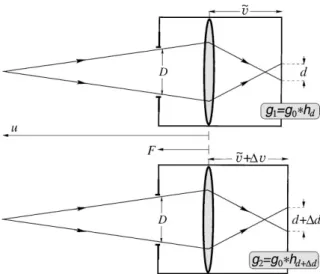
The change in the blur-diameter between the input im-ages may be achieved by changing the focus settings rather than changing the aperture size. For example, the sensor array may move axially between image acquisi-tions. We shall show that this leads to the same limita-tion as when DFD is done by changing the aperture size (Eq. (24)). We assume that geometric changes in mag-nification are compensated or do not take place (e.g. by the use of a telecentric system (Nayar et al., 1995; Watanabe and Nayar, 1996), depicted in Fig. 9). The aperture size D is constant, so in this Subsection we pa-rameterize the transfer function by the blur diameter d. Let the two images be g1 = g0 ∗hd and g2 =

Figure 9. In a telecentric system, the aperture stop is at the front focal plane. Such a system attenuates the magnification change while defocusing. Shifting the sensor position by1vcauses a change of

1d in the blur diameter.

to the known shift1v in the sensor position (Fig. 9). This change is invariant to the focus settings and the object depth in telecentric systems (Nayar et al., 1995; Schechner et al., 1998). The transfer function between the images is now

H(Eν)= Hd+1d(Eν)

Hd(ν)E . (25)

At frequencies for which |Hd(Eν)| ¿ |Hd₊₁d(Eν)| we

can take the reciprocal of Eq. (25) as the transfer func-tion between the images (in reversed order).

In Subsection 4.2 we showed that if H(ν)E is not one-to-one in d, the estimation may be ambiguous. Fig. 10 plots the response to a specific frequency ν of the 2D pillbox model (21) as a function of the blur-diameter. The figure also plots the response at the axially-displaced image (1d =1/(2ν)in this exam-ple), which is the same as the former response, but shifted along the d axis. Each ratio between these re-sponses can be yielded by many diameters d. To il-lustrate, view Fig. 11, which plots the ratio between the frequency responses in Fig. 10. The ratio is indeed not one-to-one. The lowest band for which the ratio is one-to-one in this figure is 0 < νd <1.46. How-ever, if the axial increments of the sensor position are smaller, this bandwidth broadens. As1d is decreased,

the responses shown in Fig. 10 converge. Convergence is fastest near the local extrema of Hd(ν). Hence, as 1d →0 the lowest band in which the matching

(cor-Figure 10. [Solid line] The attenuation of a frequency component

νbetween a focused and a defocused image as a function of the diameter of the blur kernel d. The horizontal axis is scaled byν. [Dashed line] The attenuation of the same frequency component when the focus settings are changed so that the blur diameter is

d+1d, for the case1d=1/(2ν).

Figure 11. Two images are acquired with different focus settings. The transfer function between the images is the ratio between their individual frequency responses, plotted in Fig. 10. In the DOF thresh-old (see Subsection 5.5)1d =1/(2ν), for which the width of the band without ambiguities satisfiesνd≈1.46. For infinitesimal1d

this width satisfiesνd≈1.63. For high frequencies or large diame-ters the width of each band isνd≈1 as in stereo.

respondence) ambiguity is avoided is between the two first local extrema, i.e.,

0< νd <1.63, (26) which is the same as Eq. (24).

Simulation and experimental results reported in Watanabe and Nayar (1996) support this theoretical result. In the DFD method suggested in Watanabe and

Nayar (1996), the defocus change between acquired images was obtained by changing the focus settings. The images were then filtered by several band pass op-erators, and the ratios of their outputs were used to fit a model. Watanabe and Nayar (1996) noticed that the solution may be ambiguous due to the unmonotonic-ity of the ratios, as a function of the frequency and the blur diameter. However, the relation to correspondence, which was related there only to stereo, was not noticed. To avoid the ambiguity they limited the band used to the first zero crossing of the pillbox model (21) which occurs atνd=1.22. However, their tests revealed that the frequency band can be extended by about 30%, i.e., toνd≈1.6, in agreement with Eq. (26). The ratio computed in Watanabe and Nayar (1996) is actually a function of the transfer function defined in Eq. (25) be-tween the images. Thus, the possibility of extending the frequency band beyond the zero crossing is not unique to the rational filter method; it is a general property of DFD.

High frequencies were not used in Watanabe and Nayar (1996) for depth estimation since they are be-yond the monotonicity cutoff. It seems that these ‘lost’ frequencies can be used in a manner similar to the coarse-to-fine approach in stereo (i.e., using the estima-tion based on low frequencies to resolve the ambiguity in the high frequencies).

4.4. DFF

We believe that by using a sufficiently large evaluation patch and some depth homogeneity within the patch, DFF is freed of the matching problem. Contrary to com-mon statements in the literature, the avoidance of the matching problem in DFF is not trivial.

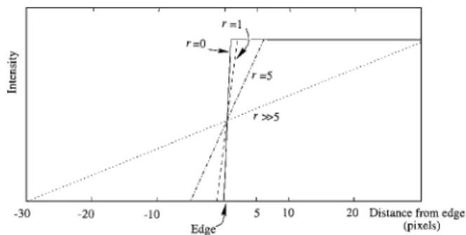
Focus measurement (like defocus and disparity mea-surements) is not a point operation. It must be calcu-lated (Jarvis, 1983; Nair and Stewart, 1992; Stewart and Nair, 1989; Subbarao and Liu, 1996) over a small patch implicitly assuming that the depth of the scene is constant (or moderately changing) within the patch (Dias et al., 1992; Marapane and Trivedi, 1993). The state of focus is detected by comparison of focus (“sharpness”) measurements in the same patch over several focus settings. To have a correct depth estima-tion, the focus measure in the patch should be largest in the focused state. The patch must be at least as large as the support of the widest blur kernel expected in the setup, otherwise errors due to edge bleeding (Nair and Stewart, 1992; Stewart and Nair, 1989) could occur (Fig. 12.). Assuming the patch to be sufficiently large,

Figure 12. Edge bleeding. The solid line shows an intensity edge. The dashed and dotted lines show the edge in pillbox-blurred images with several blur radii. The gradient at location 5−is maximal when the radius is 5 rather than 0, misleading focus detection.

we can make some observations in the frequency do-main.

Periodic images make depth from stereo ambiguous (Subsec. 4.1). They do the same to depth from vergence. As the vergence angles are changed, several vergence states yield perfect matching. On the other hand, DFF seems indeed to be immune to ambiguity due to pe-riodic input (Abbott and Ahuja, 1993; Marapane and Trivedi, 1993; Stewart and Nair, 1989). Since the blur transfer function is a LPF, the energy at any spatial fre-quency composing the image is largest at the state of focus. As the image is defocused the high-frequencies response quickly decreases (Hopkins, 1955), and de-crease in the response to other frequencies (except DC) follows. As the image is further defocused there may be local risings of the frequency response (side lobes in the response at some frequency, as a func-tion of d). However, no local maximum is as high as the response at focus in reasonable physical systems. Thus, the determination of the focused state is unam-biguous in each of the frequency components (except DC).

5. Robustness and Response to Perturbations

In some previous works, it has been empirically ob-served that DFD/DFF methods are more robust than stereo. In this section we analyze the responses of DFD, stereo and motion to perturbations, in a uni-fied framework. Some of the results depend on the characteristics of the specific model of the optical transfer function (OTF), like monotonicity and the ex-istence of zero-crossings. For defocus we use the pill-box model (Nayar et al., 1995; Noguchi and Nayar, 1994; Watanabe and Nayar, 1996), since it is valid for

aberration-free geometric optics, and has been shown to be a good approximation for large defocus (Hopkins, 1955; Lee, 1990; Schneider et al., 1994). The effects of physical optics and aberrations influence the results but one must remember that these affect also stereo and motion. Since the literature on stereo and motion neglects these effects, we maintain this assumption so as to have a common basis for comparison between stereo/motion and DFD. Nevertheless, the procedure used in this chapter is general and can serve as a guide-line in the analysis of other models.

5.1. General Error Propagation

Let us analyze the effect of a perturbation in some spa-tial frequency component of the image. The perturba-tion affects the estimated transfer funcperturba-tion between the images, which in turn causes an error in the estimated blur-diameter (DFD) or disparity (stereo). This leads to an error in the depth estimation. As in Section 4 we note that studying the behavior of each spectral component has an algorithmic ground: there are sev-eral methods (Bove, 1989; Hiura et al., 1998; Pentland, 1987; Pentland et al., 1994; Watanabe and Nayar, 1996) which rely directly on the frequency components or on frequency bands (Pentland et al., 1994) for depth es-timation. Since stereo, DFD or DFMB are based on comparison of two acquired images, we shall check the influence of a perturbation in any of the two. The problem is illustrated in Fig. 13.

The transfer function H(ν)E between the image GD

(in the frequency domain) to a reference image G0is

parameterized by the disparity/blur-diameter. We wish to estimate this parameter, for example by looking for the transfer functionH that will satisfyˆ

GD(Eν)=G0(Eν)Hˆ(ν).E (27)

Let a perturbation occur at the reference image g0. The

images are thus related by

GD(ν)E =[G0(ν)E −N0(Eν)]H(ν),E (28)

where H(ν)E is the true transfer function and N0is the

perturbation. Eqs. (27,28) yield ˆ

H(ν)E = H(Eν)−N0(ν)E H(ν)/E G0(ν)E

= H(Eν)−|N0(Eν)|

|G0(ν)E |

ejϑ(ν)E H(Eν), (29)

Figure 13. [Top]: In either of the depth estimation methods, two images are compared, where G1,G2may be G0and GD,

respec-tively, or vice versa. The comparison yields and estimate of the blur diameter/disparity, leading to the depth estimate. The relation be-tween d and u is similar for DFD/stereo/DFMB for the same system dimensions. [Bottom] A perturbation added to one of the images leads to a deviation in the estimation of d, leading to an error in the depth estimate.

whereϑ(ν)E is the phase of the perturbation relative to the signal component G0(Eν). Usually both constraints

(27,28) cannot be satisfied simultaneously at all fre-quencies, hence a common method is to minimize the MSE

E2=

Z E ν|

GD(ν)E − ˆH(ν)E G0(ν)E |2dνE

= Z

E ν|G0(Eν)|

2_{|[H(Eν)− ˆH(Eν)]−N}

0H(ν)/E G0|2dEν.

(30) This is achieved by looking for the extremum points

∂(E2₎

∂dˆ =−2Re

Z E ν|G0(ν)E |

2

·

H(ν)E − ˆH(ν)E

−N0H

G0

¸ ∂Hˆ∗(ν)E

∂dˆ dνE=0. (31)

Local minima of E2may appear at different estimates ˆ

d, for different signals and perturbations, depending on

their spectral content.

Attempting to analyze in a systematic way, let us assume that the signal is made of a single frequencyνE,

thus

G0(νE0)=D02G(ν)δ(E Eν− Eν0). (32)

If at that frequency ∂Hˆ∗(ν)/∂E dˆ = 0, the estimation of d is ill posed (or very ill conditioned). Otherwise,ˆ

nulling the integrand yields Eq. (29), which shows how the estimated frequency response changes with the in-fluence of the perturbation. FromHˆ(ν)E the parameter

ˆ

d and the depthu are derived (3). The response of theˆ

depth estimation to perturbations is ∂uˆ(Eν)

∂|N0(ν)E | =

∂uˆ

∂f(uˆ) ∂f(uˆ) ∂|N0(ν)E|,

(33)

where f(u) = d/D is as defined in Eq. (3). As we

showed in Section 2, f(u)is the same for stereo and DFD systems having the same physical dimensions, thus the factor∂u/∂f(u)is common for both systems. Hence, in the coming comparison between these ap-proaches we omit this factor and use∂f(u)/∂|N0|as

a measure for the response to perturbations. Since the estimation will be frequency-dependent, we write

∂f(uˆ,ν)E ∂|N0(Eν)| =

∂f(uˆ,ν)E ∂Hˆ(ν)E

∂Hˆ(Eν) ∂|N0|

= −ej_|ϑ(Eν)H(ν)E

G0(Eν)|

" ∂H(Eν)

∂f(u)

¯¯ ¯¯ ˆ

u

#₋1

, (34) where G0is given by Eq. (32).

Suppose now that the perturbation occurs in the transformed (shifted, or blurred) image. Eq. (28) takes the form

GD(ν)E =G0(ν)E H(ν)E +ND(ν),E (35)

while Eq. (30) changes to

E2=

Z E ν|

GD(ν)E − ˆH(ν)E G0(ν)E |2dEν

= Z

E ν|

G0(Eν)|2|[H(Eν)− ˆH(Eν)]+ND/G0|2dν.E

(36) Reasoning similar to Eqs. (29) and (31) yields

ˆ

H(ν)E =H(ν)E +|ND(ν)E |

|G0(Eν)|

ejϑ(ν)E. (37)

The response of the depth estimation to the perturbation is

∂f(uˆ,ν)E ∂|ND(Eν)| =

∂f(uˆ,ν)E ∂Hˆ(ν)E

∂Hˆ(Eν) ∂|ND|

= ejϑ(ν)E |G0(Eν)|

" ∂H(ν)E

∂f(u)

¯¯ ¯¯ ˆ

u

#−1

. (38)

5.2. Stereo—The Aperture Problem

For stereo, the transfer function H(Eν) is given by Eq. (13), so

∂fstereo(uˆ,Eν)

∂|N0(Eν)| =

ej [ϑ(Eν)−π/2]

|G(Eν)|

1 2πD₀2D

1

νcosφ, (39) ∂fstereo(uˆ,Eν)

∂|ND(ν)E | =

ej [ϑ(Eν)+π/2+2πνd cosφ]

|G(ν)E |

1 2πD2

0D

1 νcosφ.

(40) The terms in these equations express in a quantitative manner intuitive characteristics: the stronger the signal

G(Eν), the smaller is the response to the perturbation; the DC component (ν=0) contribution to the disparity es-timation is ill-posed; eses-timation by the low frequencies is ill-conditioned. The instability at the low frequen-cies stems from the fact that much larger deviations in d are needed to compensate for the perturbation,ˆ

while trying to maintain Eq. (29), than in the higher fre-quencies. Thus, Eq. (39) expresses mathematically the weakness of stereo in scenes lacking high-frequency content.

These equations also express mathematically the

aperture problem in stereo. The smaller the

compo-nent of the periodic signal along the baseline (Adelson and Wang, 1992), the larger the error is. As|φ| →π/2 we need to have D→ ∞to keep the error finite.

5.3. Motion and 1D Blur

For DFMB (analogous to 1D-DFD) the transfer func-tion is proporfunc-tional to expression (19), which has zero crossings. Perturbations in the reference image at fre-quencies/diameters for which H(ν)E = 0 influence neither the error (30) nor the depth estimation (34). Thus, if the transfer function has zero crossings (as in Castleman (1979), FitzGerrell et al. (1957), Hopkins (1955), Lee (1990), and Schneider et al. (1994), the

Figure 14. For a specificEνthe transfer function H depends on the blur-diameter. A true diameter d (larger than the monotonicity cutoff) has several solutions (e.g.dˆ1,dˆ2). Close to a peak or trough a

small deviation in the estimatedH causes a significant but boundedˆ

error (seedˆ2,dˆ3). At the high frequencies or defocus blur the transfer

function is indifferent to changes in d, thus the error may be infinite (seed vs.˜ d). Hence such frequencies would better be discarded.ˆ˜

estimation based on the zero-crossing frequencies is completely immune to noise added to the reference image, i.e.,

∂f(uˆ,ν)E ∂|N0(Eν)|

¯¯ ¯¯ ¯

H(Eν)=0, ∂_∂H_d6=0

=0. (41)

As for perturbation in the blurred image, ∂fDFMB(uˆ,ν)E

∂|ND(ν)|

¯¯ ¯¯ ¯

H(Eν)=0

= ± ejϑ(ν)E |G(ν)E |

1

D f(uˆ). (42)

Thus close to the zero crossings the results are stable even when the frequency is high.

Nevertheless, if the transfer function has zero-crossings it is not monotonous, having peaks and troughs. In these situations ∂Hˆ/∂d is locally zero,ˆ

yielding an ill conditioned estimation (see Fig. 14). Note that these are exactly the limits between the bands well posed for matching (Section 4). Assuming that a change of defocus/motion blur diameter mainly causes a scale change in H(ν)E , as in the case of the pill-box model (19), this phenomenon means that some frequencies will yield an unreliable contribution to the estimation. Still, a perturbation about a peak or trough will usually yield a bounded error since lo-cally, the range of frequencies in which∂Hˆ/∂dˆ≈0 is small.

Consider for example the peak about the DC. Substi-tuting Eq. (32) in Eq. (34), and expanding H (Eq. (19))

in a Taylor series we obtain that ∂fDFMB(uˆ,ν)E

∂|N0(Eν)|

¯¯ ¯¯ ¯

νd cosφ<1

∼ 1

D2₀D2

1

(νcosφ)2, (43)

∂fDFMB(uˆ,ν)E

∂|ND(Eν)|

¯¯ ¯¯ ¯

νd cosφ<1

∼ 1

D0D3

1

(νcosφ)2. (44)

Eqs. (43) and (44) indicate that the estimation is very unstable in the low frequencies (Subbarao et al., 1997): the response to perturbations in 1D-DFD and DFMB behaves asν−2_{in the low frequencies, and thus these}

methods are more sensitive to noise in this regime than stereo (39), for which the response behaves asν−1_{. This}

is due to the fact that DFD/DFMB use summation of rays, and wide spatial perturbations affect them most. However, since enlarging the 1D aperture enables more light to reach the sensor, the signal is stronger and thus the estimation is more stable. Thus, DFD/DFMB may outperform stereo when the aperture (baseline) is large (compared to the pinhole reference). This is due to the fact that DFD relies on numerous rays for estimation. This additional data makes the estimation potentially more robust than simple discrete triangulation. Note that according to Eq. (41) there are certain frequencies for which a perturbation does not influence the estima-tion by DFD/DFMB. As with stereo, the response to perturbation of DFMB depends on the orientationφof the spatial frequency, since the aperture problem exists also in motion.

5.4. 2D DFD

In comparison to stereo, motion and motion-blur sys-tems of the same physical dimensions, 2D-DFD re-lies on much more points in the estimation of depth (Pentland, 1987; Pentland et al., 1989; Subbarao and Wei, 1992) and is thus potentially more reliable (Farid and Simoncelli, 1998) and robust. First of all, the amount of light gathered through the large aperture is proportional to D2 _{(compared with D}

0D for DFMB,

and D2

0through a pinhole) making the signal to noise

ra-tio (Farid and Simoncelli, 1998) much higher for large apertures. Eqs. (42) and (44) take the form

∂fDFD(uˆ,Eν)

∂|ND(ν)E | = − ejϑ(Eν)

|G(ν)E |

1

D2

f(uˆ)

J2[πνD f(uˆ)]

ν_−→→∞ ejϑ(ν)E

|G(Eν)|

πf1.5(uˆ)

√ 2

√

ν

D1.5_cos[(πν_dˆ)−π/_4],

H_(ν)=0

−→ ±ejϑ(ν)E |G(Eν)|

πf1.5_(uˆ)

√ 2

1

D1_.5

√

∂fDFD(uˆ,ν)E

∂|ND(Eν)|

¯¯ ¯¯ ¯

νd<1

≈ _|ejϑ(ν)E

G(Eν)|

4

f(uˆ)π2_D4

1

ν2. (46)

To derive these relations we used ∂[J1(ξ)/ξ]

∂ξ = −

J2(ξ)

ξ (47)

and Jk(ξ)

ξ→∞

−→p2/(πξ)cos[ξ−k(π/2)−(π/4)], (48) for the circular pillbox model (21). As can be seen, in this model the error due to perturbations decreases faster with the aperture size, compared to the 1D tri-angulation methods. Here too there is instability at the very low frequencies. Indeed, to avoid the ill-posedness at the DC, in Watanabe and Nayar (1996) this component was nulled by band-pass filtering, and as a by-product the unstable contribution of the low-frequencies was suppressed.

For a circularly symmetric lens-aperture, the re-sponse is indifferent to the orientation of the fre-quency component. Hence the aperture problem does not exist.4This characteristic is valid also if the lens-aperture is not circularly symmetric, as long as it is suf-ficiently wide along both axes (the usual case). Hence, more frequencies (components of the images) may par-ticipate in the estimation by DFD and contribute sta-ble and reliasta-ble information to the estimator. There-fore DFD is potentially more robust than classic

tri-angulation methods if the system dimensions are the

same.

The indifference of the transfer function to the ori-entation of the frequency components was utilized in Pentland (1987) and Pentland et al. (1989). In that work, DFD was implemented by comparing an image acquired via a circularly symmetric large aperture to a small (“pinhole”) aperture image. Results were av-eraged over all orientations in the frequency domain, thus increasing the reliability of the estimation.

An example for the better robustness of DFD is the “monocular stereo” system presented in Simoncelli and Farid (1996), whose principle of operation is similar to that shown in Fig. 2. This was demonstrated in Farid (1997) and Farid and Simoncelli (1998). There, the same system was used for depth sensing once by dif-ferential DFD and once by difdif-ferential stereo. The

em-pirical results indeed show that the estimated depth fluctuations were significantly smaller in DFD than in stereo.

Note, that at high frequencies the estimation be-comes unstable, at a moderate rate(∼√ν). However, for other models of the OTF, it might be much more severe. Consider for example a Gaussian kernel for DFD (Nayar, 1992; Rajagopalan and Chaudhuri, 1995; Subbarao, 1988; Surya and Subbarao, 1993). Account-ing for the total light energy (as in Eqs. (15) and (16), the frequency response behaves like

HD(Eν) H0

= D2

D2 0

e−[κνD f(u)]2, (49) whereκ is a constant (real). The response to the per-turbation (38) is

∂fgauss(uˆ,ν)E

∂|ND(Eν)| = −

ejϑ(Eν)

|G(Eν)|2 f(uˆ)κ2_D4

1 ν2e

[_κνD f₍u_ˆ)]2

, (50) which is very ill conditioned in the high frequencies. This situation is also schematically described in Fig. 14: if the slope of the frequency response fromd to˜ ∞is very small, the estimation error is unbounded.

5.5. The Optimal Axial Interval in DFD

In this subsection we refer to the method considered in Subsection 4.3, where the change between the two images is achieved by changing the focus settings, in particular the axial position of the sensor. Since the aperture D is the same for all images, we parameterize the transfer function by the blur diameter d in the equa-tions to follow. Since the system has circular symmetry we use H(ν)instead of H(Eν). Let one image be (in the frequency domain)

G1(ν)=G0(ν)Hd(ν)+N1(ν), (51)

where N1(ν)is a perturbation while the other image is

G2(ν)=G0(ν)Hd+1d(ν). (52)

If there is no perturbation, the two images should satisfy the constraint

We wish to estimated by searching for the value thatˆ

will satisfy

G2(ν)Hdˆ(ν)−G1(ν)Hdˆ₊₁d(ν)=0. (54)

Similar to the discussion in Subsection 5.1, this can be satisfied for a single frequency signal. For other signals an error can be defined and minimized. Substituting Eqs. (51) and (52) into Eq. (54) yields

H_dˆ+1d(ν)Hd(ν)

=H_dˆ(ν)Hd+1d(ν)− N1(ν)

G0(ν)

H_dˆ+1d(ν). (55) Assume for a moment that Hd(ν)6=0, and define (as

in Eq. (25))

H(ν)= Hd+1d(ν)

Hd(ν) , Hˆ(ν)=

H_dˆ+1d(ν) H_dˆ(ν) . (56)

Eq. (55) can be written as ˆ

H(ν)=H(ν)

·

1+ N1(ν)

G0(ν)Hd(ν)

¸₋1

. (57)

The perturbation causes the estimated transfer function to change:

∂Hˆ(ν) ∂|N1(ν)|

= −h 1

1+ N1(ν)

G0(ν)Hd(ν)

i2

ejϑ(ν)

|G0(ν)|

Hd+1d(ν) H2

d(ν)

≈ − ejϑ(ν) |G0(ν)|

Hd+1d(ν) H2

d(ν)

, (58)

where the approximation in the right hand side of Eq. (58) is for the case that|N1(ν)|is small compared to

|G0(ν)Hd(ν)|. Similarly to Eq. (34) we seek the error

induced by the perturbation on the depth estimation. For small perturbations we assume thatHˆ(ν)≈H(ν), so

∂f(uˆ, ν) ∂|N1(ν)|

= ∂Hˆ(ν)

∂|N1(ν)|

· ·

∂Hˆ(ν) ∂f(uˆ)

¸₋1

≈ − ejϑ(ν) |G(ν)|D2

0

Hd₊₁d(ν) D∂Hd+1d(ν)

∂d Hd(ν)−D∂ Hd(ν)

∂d Hd+1d(ν) . (59)

According to Eqs. (58) and (59), if Hd+1d(ν)=0 for this frequency, a perturbation N1 does not affect the

estimation.

If|Hd(ν)| ¿ |Hd₊₁d(ν)|we define the transfer

func-tion between the images as the reciprocal of Eq. (56):

H−1(ν)= Hd(ν) Hd₊₁d(ν)

, Hd−1(ν)= Hdˆ(ν) H_dˆ+1d(ν).

(60) This takes care of the cases in which Hd(ν) = 0 but Hd+1d(ν)6=0. Eq. (55) can be written as

d

H−1(ν)=_H−1_(ν)+ N1(ν)

G0(ν)Hd+1d(ν)

. (61)

The perturbation causes the estimated transfer function to change:

∂Hd−1(ν)

∂|N1(ν)|

= _| ejϑ(ν)

G0(ν)|Hd+1d(ν)

. (62)

Calculating the influence on the depth estimation based on this transfer function, we arrive at the same relation as Eq. (59). Thus, we do not need to assume that|N1(ν)|

is small compared to|G0(ν)Hd(ν)|.

In the pillbox model we use Eq. (23), and Eq. (59) takes a relatively simple form,

≈_2|ejϑ(ν)

G(ν)| f(u)

D2

× J1[πν(d+1d)]

J2[πν(d+1d)]J1(πνd)−J2(πνd)J1[πν(d+1d)]

(63) which at the high frequencies (or defocus) becomes (48)

∂f(uˆ, ν) ∂|N1(ν)|

≈ _|ejϑ(ν)

G(ν)| πd√νd

D3₂√₂

sin[πν(d+1d)−(π/4)]

sin(πν1d) .

(64) A similar relation is obtained in case a perturbation N2

is present in G2rather than in G1:

∂f(uˆ, ν) ∂|N2(ν)|

≈ −_|ejϑ(ν)

G(ν)|

π(d+1d)√ν(d+1d) D3₂√₂

×sin[πνd−(π/4)]