Basics of Compiler Design

(1)

Basics of Compiler Design

Anniversary edition

Torben Ægidius Mogensen

DEPARTMENT OF COMPUTER SCIENCE UNIVERSITY OF COPENHAGEN

(2)

c

Torben Ægidius Mogensen 2000 – 2010

[email protected]

Department of Computer Science University of Copenhagen Universitetsparken 1 DK-2100 Copenhagen DENMARK

Book homepage:

http://www.diku.dk/∼torbenm/Basics

First published 2000

This edition: August 20, 2010

(3)

List of Figures

2.1 Regular expressions . . . 11

2.2 Some algebraic properties of regular expressions . . . 14

2.3 Example of an NFA . . . 17

2.4 Constructing NFA fragments from regular expressions . . . 19

2.5 NFA for the regular expression (a|b)∗ac . . . 20

2.6 Optimised NFA construction for regular expression shorthands . . 21

2.7 Optimised NFA for[0-9]+ . . . 21

2.8 Example of a DFA . . . 22

2.9 DFA constructed from the NFA in figure 2.5 . . . 29

2.10 Non-minimal DFA . . . 32

2.11 Minimal DFA . . . 34

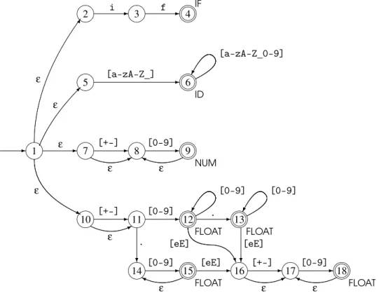
2.12 Combined NFA for several tokens . . . 38

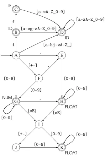
2.13 Combined DFA for several tokens . . . 39

2.14 A 4-state NFA that gives 15 DFA states . . . 44

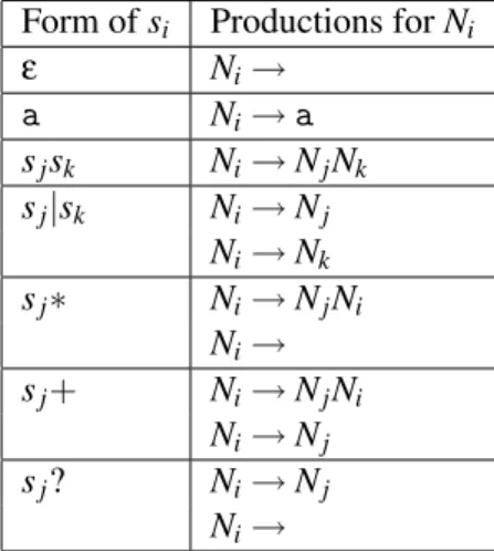
3.1 From regular expressions to context free grammars . . . 56

3.2 Simple expression grammar . . . 57

3.3 Simple statement grammar . . . 57

3.4 Example grammar . . . 59

3.5 Derivation of the stringaabbbccusing grammar 3.4 . . . 59

3.6 Leftmost derivation of the stringaabbbccusing grammar 3.4 . . . 59

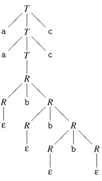
3.7 Syntax tree for the stringaabbbccusing grammar 3.4 . . . 61

3.8 Alternative syntax tree for the stringaabbbccusing grammar 3.4 . 61 3.9 Unambiguous version of grammar 3.4 . . . 62

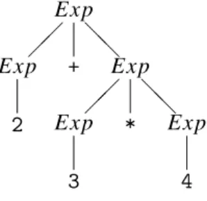
3.10 Preferred syntax tree for2+3*4using grammar 3.2 . . . 63

3.11 Unambiguous expression grammar . . . 66

3.12 Syntax tree for2+3*4using grammar 3.11 . . . 67

3.13 Unambiguous grammar for statements . . . 68

3.14 Fixed-point iteration for calculation ofNullable . . . 71

3.15 Fixed-point iteration for calculation ofFIRST . . . 72

3.16 Recursive descent parser for grammar 3.9 . . . 81

(10)

3.17 LL(1) table for grammar 3.9 . . . 82

3.18 Program for table-driven LL(1) parsing . . . 83

3.19 Input and stack during table-driven LL(1) parsing . . . 83

3.20 Removing left-recursion from grammar 3.11 . . . 85

3.21 Left-factorised grammar for conditionals . . . 87

3.22 SLR table for grammar 3.9 . . . 90

3.23 Algorithm for SLR parsing . . . 91

3.24 Example SLR parsing . . . 91

3.25 Example grammar for SLR-table construction . . . 92

3.26 NFAs for the productions in grammar 3.25 . . . 92

3.27 Epsilon-transitions added to figure 3.26 . . . 93

3.28 SLR DFA for grammar 3.9 . . . 94

3.29 Summary of SLR parse-table construction . . . 95

3.30 Textual representation of NFA states . . . 103

5.1 Example language for interpretation . . . 123

5.2 Evaluating expressions . . . 125

5.3 Evaluating a function call . . . 127

5.4 Interpreting a program . . . 128

6.1 The design space of types . . . 134

6.2 Type checking of expressions . . . 137

6.3 Type checking a function declaration . . . 139

6.4 Type checking a program . . . 141

7.1 The intermediate language . . . 150

7.2 A simple expression language . . . 152

7.3 Translating an expression . . . 154

7.4 Statement language . . . 156

7.5 Translation of statements . . . 158

7.6 Translation of simple conditions . . . 159

7.7 Example language with logical operators . . . 161

7.8 Translation of sequential logical operators . . . 162

7.9 Translation for one-dimensional arrays . . . 166

7.10 A two-dimensional array . . . 168

7.11 Translation of multi-dimensional arrays . . . 169

7.12 Translation of simple declarations . . . 173

8.1 Pattern/replacement pairs for a subset of the MIPS instruction set . 185 9.1 Gen and kill sets . . . 194

(11)

LIST OF FIGURES ix

9.3 succ,genandkillfor the program in figure 9.2 . . . 196

9.4 Fixed-point iteration for liveness analysis . . . 197

9.5 Interference graph for the program in figure 9.2 . . . 198

9.6 Algorithm 9.3 applied to the graph in figure 9.5 . . . 202

9.7 Program from figure 9.2 after spilling variablea . . . 203

9.8 Interference graph for the program in figure 9.7 . . . 203

9.9 Colouring of the graph in figure 9.8 . . . 204

10.1 Simple activation record layout . . . 211

10.2 Prologue and epilogue for the frame layout shown in figure 10.1 . 212 10.3 Call sequence forx:=CALL f(a₁, . . . ,an) using the frame layout shown in figure 10.1 . . . 213

10.4 Activation record layout for callee-saves . . . 214

10.5 Prologue and epilogue for callee-saves . . . 214

10.6 Call sequence forx:=CALL f(a1, . . . ,an)for callee-saves . . . 215

10.7 Possible division of registers for 16-register architecture . . . 216

10.8 Activation record layout for the register division shown in figure 10.7216 10.9 Prologue and epilogue for the register division shown in figure 10.7 217 10.10Call sequence forx:=CALL f(a1, . . . ,an)for the register division shown in figure 10.7 . . . 218

10.11Example of nested scopes in Pascal . . . 223

10.12Adding an explicit frame-pointer to the program from figure 10.11 224 10.13Activation record with static link . . . 225

10.14Activation records forfandgfrom figure 10.11 . . . 225

11.1 Gen and kill sets for available assignments . . . 235

11.2 Example program for available-assignments analysis . . . 236

11.3 pred,genandkillfor the program in figure 11.2 . . . 237

11.4 Fixed-point iteration for available-assignment analysis . . . 238

11.5 The program in figure 11.2 after common subexpression elimination. 239 11.6 Equations for index-check elimination . . . 242

11.7 Intermediate code for for-loop with index check . . . 244

(12)

(13)

Chapter 1

Introduction

1.1 What is a compiler?

In order to reduce the complexity of designing and building computers, nearly all of these are made to execute relatively simple commands (but do so very quickly). A program for a computer must be built by combining these very simple commands into a program in what is calledmachine language. Since this is a tedious and error-prone process most programming is, instead, done using a high-levelprogramming language. This language can be very different from the machine language that the computer can execute, so some means of bridging the gap is required. This is where thecompilercomes in.

A compiler translates (orcompiles) a program written in a high-level program-ming language that is suitable for human programmers into the low-level machine language that is required by computers. During this process, the compiler will also attempt to spot and report obvious programmer mistakes.

Using a high-level language for programming has a large impact on how fast programs can be developed. The main reasons for this are:

• Compared to machine language, the notation used by programming lan-guages is closer to the way humans think about problems.

• The compiler can spot some obvious programming mistakes.

• Programs written in a high-level language tend to be shorter than equivalent programs written in machine language.

Another advantage of using a high-level level language is that the same program can be compiled to many different machine languages and, hence, be brought to run on many different machines.

(14)

On the other hand, programs that are written in a high-level language and auto-matically translated to machine language may run somewhat slower than programs that are hand-coded in machine language. Hence, some time-critical programs are still written partly in machine language. A good compiler will, however, be able to get very close to the speed of hand-written machine code when translating well-structured programs.

1.2 The phases of a compiler

Since writing a compiler is a nontrivial task, it is a good idea to structure the work. A typical way of doing this is to split the compilation into several phases with well-defined interfaces. Conceptually, these phases operate in sequence (though in practice, they are often interleaved), each phase (except the first) taking the output from the previous phase as its input. It is common to let each phase be handled by a separate module. Some of these modules are written by hand, while others may be generated from specifications. Often, some of the modules can be shared between several compilers.

A common division into phases is described below. In some compilers, the ordering of phases may differ slightly, some phases may be combined or split into several phases or some extra phases may be inserted between those mentioned be-low.

Lexical analysis This is the initial part of reading and analysing the program text: The text is read and divided intotokens, each of which corresponds to a sym-bol in the programming language,e.g., a variable name, keyword or number. Syntax analysis This phase takes the list of tokens produced by the lexical analysis and arranges these in a tree-structure (called thesyntax tree) that reflects the structure of the program. This phase is often calledparsing.

Type checking This phase analyses the syntax tree to determine if the program violates certain consistency requirements,e.g., if a variable is used but not declared or if it is used in a context that does not make sense given the type of the variable, such as trying to use a boolean value as a function pointer. Intermediate code generation The program is translated to a simple

machine-independent intermediate language.

Register allocation The symbolic variable names used in the intermediate code are translated to numbers, each of which corresponds to a register in the target machine code.

(15)

1.3. INTERPRETERS 3 Machine code generation The intermediate language is translated to assembly language (a textual representation of machine code) for a specific machine architecture.

Assembly and linking The assembly-language code is translated into binary rep-resentation and addresses of variables, functions,etc., are determined. The first three phases are collectively calledthe frontendof the compiler and the last three phases are collectively calledthe backend. The middle part of the compiler is in this context only the intermediate code generation, but this often includes various optimisations and transformations on the intermediate code.

Each phase, through checking and transformation, establishes stronger invari-ants on the things it passes on to the next, so that writing each subsequent phase is easier than if these have to take all the preceding into account. For example, the type checker can assume absence of syntax errors and the code generation can assume absence of type errors.

Assembly and linking are typically done by programs supplied by the machine or operating system vendor, and are hence not part of the compiler itself, so we will not further discuss these phases in this book.

1.3 Interpreters

Aninterpreteris another way of implementing a programming language.

Interpre-tation shares many aspects with compiling. Lexing, parsing and type-checking are in an interpreter done just as in a compiler. But instead of generating code from the syntax tree, the syntax tree is processed directly to evaluate expressions and execute statements, and so on. An interpreter may need to process the same piece of the syntax tree (for example, the body of a loop) many times and, hence, inter-pretation is typically slower than executing a compiled program. But writing an interpreter is often simpler than writing a compiler and the interpreter is easier to move to a different machine (see chapter 13), so for applications where speed is not of essence, interpreters are often used.

Compilation and interpretation may be combined to implement a programming language: The compiler may produce intermediate-level code which is then inter-preted rather than compiled to machine code. In some systems, there may even be parts of a program that are compiled to machine code, some parts that are compiled to intermediate code, which is interpreted at runtime while other parts may be kept as a syntax tree and interpreted directly. Each choice is a compromise between speed and space: Compiled code tends to be bigger than intermediate code, which tend to be bigger than syntax, but each step of translation improves running speed. Using an interpreter is also useful during program development, where it is more important to be able to test a program modification quickly rather than run

(16)

the program efficiently. And since interpreters do less work on the program before execution starts, they are able to start running the program more quickly. Further-more, since an interpreter works on a representation that is closer to the source code than is compiled code, error messages can be more precise and informative.

We will discuss interpreters briefly in chapters 5 and 13, but they are not the main focus of this book.

1.4 Why learn about compilers?

Few people will ever be required to write a compiler for a general-purpose language like C, Pascal or SML. So why do most computer science institutions offer compiler courses and often make these mandatory?

Some typical reasons are:

a) It is considered a topic that you should know in order to be “well-cultured” in computer science.

b) A good craftsman should know his tools, and compilers are important tools for programmers and computer scientists.

c) The techniques used for constructing a compiler are useful for other purposes as well.

d) There is a good chance that a programmer or computer scientist will need to write a compiler or interpreter for a domain-specific language.

The first of these reasons is somewhat dubious, though something can be said for “knowing your roots”, even in such a hastily changing field as computer science.

Reason “b” is more convincing: Understanding how a compiler is built will al-low programmers to get an intuition about what their high-level programs will look like when compiled and use this intuition to tune programs for better efficiency. Furthermore, the error reports that compilers provide are often easier to understand when one knows about and understands the different phases of compilation, such as knowing the difference between lexical errors, syntax errors, type errors and so on.

The third reason is also quite valid. In particular, the techniques used for read-ing (lexread-ingandparsing) the text of a program and converting this into a form (ab-stract syntax) that is easily manipulated by a computer, can be used to read and manipulate any kind of structured text such as XML documents, address lists,etc.. Reason “d” is becoming more and more important as domain specific languages (DSLs) are gaining in popularity. A DSL is a (typically small) language designed for a narrow class of problems. Examples are data-base query languages, text-formatting languages, scene description languages for ray-tracers and languages

(17)

1.5. THE STRUCTURE OF THIS BOOK 5 for setting up economic simulations. The target language for a compiler for a DSL may be traditional machine code, but it can also be another high-level language for which compilers already exist, a sequence of control signals for a machine, or formatted text and graphics in some printer-control language (e.g. PostScript). Even so, all DSL compilers will share similar front-ends for reading and analysing the program text.

Hence, the methods needed to make a compiler front-end are more widely ap-plicable than the methods needed to make a compiler back-end, but the latter is more important for understanding how a program is executed on a machine.

1.5 The structure of this book

The first part of the book describes the methods and tools required to read program text and convert it into a form suitable for computer manipulation. This process is made in two stages: A lexical analysis stage that basically divides the input text into a list of “words”. This is followed by a syntax analysis (or parsing) stage that analyses the way these words form structures and converts the text into a data structure that reflects the textual structure. Lexical analysis is covered in chapter 2 and syntactical analysis in chapter 3.

The second part of the book (chapters 4 – 10) covers the middle part and back-end of interpreters and compilers. Chapter 4 covers how definitions and uses of names (identifiers) are connected throughsymbol tables. Chapter 5 shows how you can implement a simple programming language by writing an interpreter and notes that this gives a considerable overhead that can be reduced by doing more things be-fore executing the program, which leads to the following chapters about static type checking (chapter 6) and compilation (chapters 7 – 10. In chapter 7, it is shown how expressions and statements can be compiled into an intermediate language, a language that is close to machine language but hides machine-specific details. In chapter 8, it is discussed how the intermediate language can be converted into “real” machine code. Doing this well requires that the registers in the processor are used to store the values of variables, which is achieved by aregister allocation process, as described in chapter 9. Up to this point, a “program” has been what corresponds to the body of a single procedure. Procedure calls and nested proce-dure declarations add some issues, which are discussed in chapter 10. Chapter 11 deals with analysis and optimisation and chapter 12 is about allocating and freeing memory. Finally, chapter 13 will discuss the process ofbootstrappinga compiler, i.e., using a compiler to compile itself.

The book uses standard set notation and equations over sets. Appendix A con-tains a short summary of these, which may be helpful to those that need these concepts refreshed.

(18)

(about interpreters) was added in 2009, which is why editions after April 2008 are called “extended”. In the 2010 edition, further additions (including chapter 12 and appendix A) were made. Since ten years have passed since the first edition was printed as lecture notes, the 2010 edition is labeled “anniversary edition”.

1.6 To the lecturer

This book was written for use in the introductory compiler course at DIKU, the department of computer science at the University of Copenhagen, Denmark.

At DIKU, the compiler course was previously taught right after the introduc-tory programming course, which is earlier than in most other universities. Hence, existing textbooks tended either to be too advanced for the level of the course or be too simplistic in their approach, for example only describing a single very simple compiler without bothering too much with the general picture.

This book was written as a response to this and aims at bridging the gap: It is intended to convey the general picture without going into extreme detail about such things as efficient implementation or the newest techniques. It should give the students an understanding of how compilers work and the ability to make simple (but not simplistic) compilers for simple languages. It will also lay a foundation that can be used for studying more advanced compilation techniques, as founde.g. in [35]. The compiler course at DIKU was later moved to the second year, so additions to the original text has been made.

At times, standard techniques from compiler construction have been simplified for presentation in this book. In such cases references are made to books or articles where the full version of the techniques can be found.

The book aims at being “language neutral”. This means two things:

• Little detail is given about how the methods in the book can be implemented in any specific language. Rather, the description of the methods is given in the form of algorithm sketches and textual suggestions of how these can be implemented in various types of languages, in particular imperative and functional languages.

• There is no single through-going example of a language to be compiled. In-stead, different small (sub-)languages are used in various places to cover ex-actly the points that the text needs. This is done to avoid drowning in detail, hopefully allowing the readers to “see the wood for the trees”.

Each chapter (except this) has a section on further reading, which suggests additional reading material for interested students. All chapters (also except this) has a set of exercises. Few of these require access to a computer, but can be solved on paper or black-board. In fact, many of the exercises are based on exercises that

(19)

1.7. ACKNOWLEDGEMENTS 7 have been used in written exams at DIKU. After some of the sections in the book, a few easy exercises are listed. It is suggested that the student attempts to solve these exercises before continuing reading, as the exercises support understanding of the previous sections.

Teaching with this book can be supplemented with project work, where students write simple compilers. Since the book is language neutral, no specific project is given. Instead, the teacher must choose relevant tools and select a project that fits the level of the students and the time available. Depending on how much of the book is used and the amount of project work, the book can support course sizes ranging from 5 to 15 ECTS points.

1.7 Acknowledgements

The author wishes to thank all people who have been helpful in making this book a reality. This includes the students who have been exposed to draft versions of the book at the compiler courses “Dat 1E” and “Oversættere” at DIKU, and who have found numerous typos and other errors in the earlier versions. I would also like to thank the instructors at Dat 1E and Oversættere, who have pointed out places where things were not as clear as they could be. I am extremely grateful to the people who in 2000 read parts of or all of the first draft and made helpful suggestions.

1.8 Permission to use

Permission to copy and print for personal use is granted. If you, as a lecturer, want to print the book and sell it to your students, you can do so if you only charge the printing cost. If you want to print the book and sell it at profit, please contact the author [email protected] we will find a suitable arrangement.

In all cases, if you find any misprints or other errors, please contact the author [email protected].

(20)

(21)

Chapter 2

Lexical Analysis

2.1 Introduction

The word “lexical” in the traditional sense means “pertaining to words”. In terms of programming languages, words are objects like variable names, numbers, keywords etc. Such words are traditionally calledtokens.

Alexical analyser, orlexerfor short, will as its input take a string of individual letters and divide this string into tokens. Additionally, it will filter out whatever separates the tokens (the so-called white-space), i.e., lay-out characters (spaces, newlinesetc.) and comments.

The main purpose of lexical analysis is to make life easier for the subsequent syntax analysis phase. In theory, the work that is done during lexical analysis can be made an integral part of syntax analysis, and in simple systems this is indeed often done. However, there are reasons for keeping the phases separate:

• Efficiency: A lexer may do the simple parts of the work faster than the more general parser can. Furthermore, the size of a system that is split in two may be smaller than a combined system. This may seem paradoxical but, as we shall see, there is a non-linear factor involved which may make a separated system smaller than a combined system.

• Modularity: The syntactical description of the language need not be cluttered with small lexical details such as white-space and comments.

• Tradition: Languages are often designed with separate lexical and syntacti-cal phases in mind, and the standard documents of such languages typisyntacti-cally separate lexical and syntactical elements of the languages.

It is usually not terribly difficult to write a lexer by hand: You first read past initial white-space, then you, in sequence, test to see if the next token is a keyword, a

(22)

number, a variable or whatnot. However, this is not a very good way of handling the problem: You may read the same part of the input repeatedly while testing each possible token and in some cases it may not be clear where the next token ends. Furthermore, a handwritten lexer may be complex and difficult to main-tain. Hence, lexers are normally constructed bylexer generators, which transform human-readable specifications of tokens and white-space into efficient programs.

We will see the same general strategy in the chapter about syntax analysis: Specifications in a well-defined human-readable notation are transformed into effi-cient programs.

For lexical analysis, specifications are traditionally written using regular ex-pressions: An algebraic notation for describing sets of strings. The generated lexers are in a class of extremely simple programs calledfinite automata.

This chapter will describe regular expressions and finite automata, their prop-erties and how regular expressions can be converted to finite automata. Finally, we discuss some practical aspects of lexer generators.

2.2 Regular expressions

The set of all integer constants or the set of all variable names are sets of strings, where the individual letters are taken from a particular alphabet. Such a set of strings is called alanguage. For integers, the alphabet consists of the digits 0-9 and for variable names the alphabet contains both letters and digits (and perhaps a few other characters, such as underscore).

Given an alphabet, we will describe sets of strings byregular expressions, an algebraic notation that is compact and easy for humans to use and understand. The idea is that regular expressions that describe simple sets of strings can be combined to form regular expressions that describe more complex sets of strings.

When talking about regular expressions, we will use the letters (r, sandt) in italics to denote unspecified regular expressions. When letters stand for themselves (i.e., in regular expressions that describe strings that use these letters) we will use typewriter font, e.g., a or b. Hence, when we say, e.g., “The regular expression s” we mean the regular expression that describes a single one-letter string “s”, but when we say “The regular expressions”, we mean a regular expression of any form which we just happen to calls. We use the notation L(s) to denote the language (i.e., set of strings) described by the regular expressions. For example, L(a) is the set {“a”}.

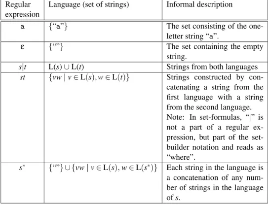
Figure 2.1 shows the constructions used to build regular expressions and the languages they describe:

• A single letter describes the language that has the one-letter string consisting of that letter as its only element.

(23)

2.2. REGULAR EXPRESSIONS 11

Regular expression

Language (set of strings) Informal description

a {“a”} The set consisting of the

one-letter string “a”.

ε {“”} The set containing the empty

string.

s|t L(s)∪L(t) Strings from both languages st {vw|v∈L(s),w∈L(t)} Strings constructed by

con-catenating a string from the first language with a string from the second language. Note: In set-formulas, “|” is not a part of a regular ex-pression, but part of the set-builder notation and reads as “where”.

s∗ {“”} ∪ {vw|v∈L(s),w∈L(s∗)} Each string in the language is a concatenation of any num-ber of strings in the language ofs.

(24)

• The symbolε(the Greek letterepsilon) describes the language that consists

solely of the empty string. Note that this is not the empty set of strings (see exercise 2.10).

• s|t(pronounced “sort”) describes the union of the languages described bys andt.

• st(pronounced “s t”) describes the concatenation of the languages L(s) and L(t),i.e., the sets of strings obtained by taking a string from L(s) and putting this in front of a string from L(t). For example, if L(s) is {“a”, “b”} and L(t) is {“c”, “d”}, then L(st) is the set {“ac”, “ad”, “bc”, “bd”}.

• The language fors∗(pronounced “sstar”) is described recursively: It consists of the empty string plus whatever can be obtained by concatenating a string from L(s) to a string from L(s∗). This is equivalent to saying that L(s∗) con-sists of strings that can be obtained by concatenating zero or more (possibly different) strings from L(s). If, for example, L(s) is {“a”, “b”} then L(s∗) is {“”, “a”, “b”, “aa”, “ab”, “ba”, “bb”, “aaa”, . . . },i.e., any string (including the empty) that consists entirely ofas andbs.

Note that while we use the same notation for concrete strings and regular expres-sions denoting one-string languages, the context will make it clear which is meant. We will often show strings and sets of strings without using quotation marks,e.g., write {a,bb} instead of {“a”, “bb”}. When doing so, we will useεto denote the

empty string, so the example from L(s∗) above is written as {ε,a,b,aa,ab,ba,bb, aaa, . . . }. The lettersu, vandwin italics will be used to denote unspecified single strings,i.e., members of some language. As an example,abwdenotes any string starting withab.

Precedence rules

When we combine different constructor symbols, e.g., in the regular expression a|ab∗, it is not a priori clear how the different subexpressions are grouped. We can use parentheses to make the grouping of symbols explicit such as in (a|(ab))∗. Additionally, we use precedence rules, similar to the algebraic convention that 3+

4∗5 means 3 added to the product of 4 and 5 and not multiplying the sum of 3 and 4 by 5. For regular expressions, we use the following conventions: ∗ binds tighter than concatenation, which binds tighter than alternative (|). The example a|ab∗from above, hence, is equivalent toa|(a(b∗)).

The |operator is associative and commutative (as it corresponds to set union, which has these properties). Concatenation is associative (but obviously not com-mutative) and distributes over|. Figure 2.2 shows these and other algebraic

(25)

prop-2.2. REGULAR EXPRESSIONS 13 erties of regular expressions, including definitions of some of the shorthands intro-duced below.

2.2.1 Shorthands

While the constructions in figure 2.1 suffice to describe e.g., number strings and variable names, we will often use extra shorthands for convenience. For example, if we want to describe non-negative integer constants, we can do so by saying that it is one or more digits, which is expressed by the regular expression

(0|1|2|3|4|5|6|7|8|9)(0|1|2|3|4|5|6|7|8|9)∗

The large number of different digits makes this expression rather verbose. It gets even worse when we get to variable names, where we must enumerate all alphabetic letters (in both upper and lower case).

Hence, we introduce a shorthand for sets of letters. Sequences of letters within square brackets represent the set of these letters. For example, we use [ab01] as a shorthand fora|b|0|1. Additionally, we can use interval notation to abbreviate [0123456789] to [0-9]. We can combine several intervals within one bracket and for example write [a-zA-Z] to denote all alphabetic letters in both lower and upper case.

When using intervals, we must be aware of the ordering for the symbols in-volved. For the digits and letters used above, there is usually no confusion. How-ever, if we write,e.g., [0-z] it is not immediately clear what is meant. When using such notation in lexer generators, standard ASCII or ISO 8859-1 character sets are usually used, with the hereby implied ordering of symbols. To avoid confusion, we will use the interval notation only for intervals of digits or alphabetic letters.

Getting back to the example of integer constants above, we can now write this much shorter as [0-9][0-9]∗.

Since s∗ denotes zero or more occurrences of s, we needed to write the set of digits twice to describe that one or more digits are allowed. Such non-zero repetition is quite common, so we introduce another shorthand,s+, to denote one or more occurrences ofs. With this notation, we can abbreviate our description of integers to [0-9]+. On a similar note, it is common that we can have zero or one occurrence of something (e.g., an optional sign to a number). Hence we introduce the shorthands? fors|ε. +and ? bind with the same precedence as∗.

We must stress that these shorthands are just that. They do not add anything to the set of languages we can describe, they just make it possible to describe a language more compactly. In the case of s+, it can even make an exponential difference: If + is nested n deep, recursive expansion ofs+ toss∗ yields 2n−1 occurrences of∗in the expanded regular expression.

(26)

(r|s)|t = r|s|t = r|(s|t) |is associative s|t = t|s |is commutative

s|s = s |is idempotent s? = s|ε by definition

(rs)t = rst = r(st) concatenation is associative

sε = s = εs εis a neutral element for concatenation

r(s|t) = rs|rt concatenation distributes over|

(r|s)t = rt|st concatenation distributes over|

(s∗)∗ = s∗ ∗is idempotent

s∗s∗ = s∗ 0 or more twice is still 0 or more ss∗ = s+ = s∗s by definition

Figure 2.2: Some algebraic properties of regular expressions

2.2.2 Examples

We have already seen how we can describe non-negative integer constants using regular expressions. Here are a few examples of other typical programming lan-guage elements:

Keywords. A keyword likeifis described by a regular expression that looks ex-actly like that keyword,e.g., the regular expressionif(which is the concatenation of the two regular expressionsiandf).

Variable names. In the programming language C, a variable name consists of letters, digits and the underscore symbol and it must begin with a letter or under-score. This can be described by the regular expression

[a-zA-Z_][a-zA-Z_0-9]∗.

Integers. An integer constant is an optional sign followed by a non-empty se-quence of digits: [+-]?[0-9]+. In some languages, the sign is a separate symbol and not part of the constant itself. This will allow whitespace between the sign and the number, which is not possible with the above.

Floats. A floating-point constant can have an optional sign. After this, the man-tissa part is described as a sequence of digits followed by a decimal point and then

(27)

2.3. NONDETERMINISTIC FINITE AUTOMATA 15 another sequence of digits. Either one (but not both) of the digit sequences can be empty. Finally, there is an optional exponent part, which is the lettere(in upper or lower case) followed by an (optionally signed) integer constant. If there is an ex-ponent part to the constant, the mantissa part can be written as an integer constant (i.e., without the decimal point). Some examples:

3.14 -3. .23 3e+4 11.22e-3.

This rather involved format can be described by the following regular expres-sion:

[+-]?((([0-9]+.[0-9]∗|.[0-9]+)([eE][+-]?[0-9]+)?)|[0-9]+[eE][+-]?[0-9]+)

This regular expression is complicated by the fact that the exponent is optional if the mantissa contains a decimal point, but not if it does not (as that would make the number an integer constant). We can make the description simpler if we make the regular expression for floats also include integers, and instead use other means of distinguishing integers from floats (see section 2.9 for details). If we do this, the regular expression can be simplified to

[+-]?(([0-9]+(.[0-9]∗)?|.[0-9]+)([eE][+-]?[0-9]+)?)

String constants. A string constant starts with a quotation mark followed by a sequence of symbols and finally another quotation mark. There are usually some restrictions on the symbols allowed between the quotation marks. For example, line-feed characters or quotes are typically not allowed, though these may be rep-resented by special “escape” sequences of other characters, such as"\n\n"for a string containing two line-feeds. As a (much simplified) example, we can by the following regular expression describe string constants where the allowed symbols are alphanumeric characters and sequences consisting of the backslash symbol fol-lowed by a letter (where each such pair is intended to represent a non-alphanumeric symbol):

"([a-zA-Z0-9]|\[a-zA-Z])∗" Suggested exercises: 2.1, 2.10(a).

2.3 Nondeterministic finite automata

In our quest to transform regular expressions into efficient programs, we use a stepping stone: Nondeterministic finite automata. By their nondeterministic nature, these are not quite as close to “real machines” as we would like, so we will later see how these can be transformed intodeterministicfinite automata, which are easily and efficiently executable on normal hardware.

(28)

A finite automaton is, in the abstract sense, a machine that has a finite number ofstates and a finite number of transitionsbetween these. A transition between states is usually labelled by a character from the input alphabet, but we will also use transitions marked withε, the so-calledepsilon transitions.

A finite automaton can be used to decide if an input string is a member in some particular set of strings. To do this, we select one of the states of the automaton as thestarting state. We start in this state and in each step, we can do one of the following:

• Follow an epsilon transition to another state, or

• Read a character from the input and follow a transition labelled by that char-acter.

When all characters from the input are read, we see if the current state is marked as beingaccepting. If so, the string we have read from the input is in the language defined by the automaton.

We may have a choice of several actions at each step: We can choose between either an epsilon transition or a transition on an alphabet character, and if there are several transitions with the same symbol, we can choose between these. This makes the automatonnondeterministic, as the choice of action is not determined solely by looking at the current state and input. It may be that some choices lead to an accepting state while others do not. This does, however, not mean that the string is sometimes in the language and sometimes not: We will include a string in the language if it ispossibleto make a sequence of choices that makes the string lead to an accepting state.

You can think of it as solving a maze with symbols written in the corridors. If you can find the exit while walking over the letters of the string in the correct order, the string is recognized by the maze.

We can formally define a nondeterministic finite automaton by:

Definition 2.1 A nondeterministic finite automaton consists of a set S of states. One of these states, s₀∈S, is called thestarting stateof the automaton and a subset F⊆S of the states areaccepting states. Additionally, we have a set T oftransitions. Each transition t connects a pair of states s1and s2and is labelled with a symbol, which is either a character c from the alphabetΣ, or the symbolε, which indicates

anepsilon-transition. A transition from state s to state t on the symbol c is written as sct.

Starting states are sometimes calledinitial statesand accepting states can also be calledfinal states(which is why we use the letterF to denote the set of accepting states). We use the abbreviations FA for finite automaton, NFA for nondeterministic finite automaton and (later in this chapter) DFA for deterministic finite automaton.

(29)

2.3. NONDETERMINISTIC FINITE AUTOMATA 17 We will mostly use a graphical notation to describe finite automata. States are denoted by circles, possibly containing a number or name that identifies the state. This name or number has, however, no operational significance, it is solely used for identification purposes. Accepting states are denoted by using a double circle instead of a single circle. The initial state is marked by an arrow pointing to it from outside the automaton.

A transition is denoted by an arrow connecting two states. Near its midpoint, the arrow is labelled by the symbol (possiblyε) that triggers the transition. Note

that the arrow that marks the initial state isnota transition and is, hence, not marked by a symbol.

Repeating the maze analogue, the circles (states) are rooms and the arrows (transitions) are one-way corridors. The double circles (accepting states) are exits, while the unmarked arrow to the starting state is the entrance to the maze.

Figure 2.3 shows an example of a nondeterministic finite automaton having three states. State 1 is the starting state and state 3 is accepting. There is an epsilon-transition from state 1 to state 2, epsilon-transitions on the symbolafrom state 2 to states 1 and 3 and a transition on the symbolbfrom state 1 to state 3. This NFA recognises the language described by the regular expressiona∗(a|b). As an example, the string aabis recognised by the following sequence of transitions:

from to by

1 2 ε

2 1 a

1 2 ε

2 1 a

1 3 b

At the end of the input we are in state 3, which is accepting. Hence, the string is accepted by the NFA. You can check this by placing a coin at the starting state and follow the transitions by moving the coin.

Note that we sometimes have a choice of several transitions. If we are in state

1 b

ε

3

2 a

? a

(30)

2 and the next symbol is an a, we can, when reading this, either go to state 1 or to state 3. Likewise, if we are in state 1 and the next symbol is ab, we can either read this and go to state 3 or we can use the epsilon transition to go directly to state 2 without reading anything. If we in the example above had chosen to follow thea-transition to state 3 instead of state 1, we would have been stuck: We would have no legal transition and yet we would not be at the end of the input. But, as previously stated, it is enough that thereexistsa path leading to acceptance, so the stringaabis still accepted.

A program that decides if a string is accepted by a given NFA will have to check all possible paths to see ifanyof these accepts the string. This requires either backtracking until a successful path found or simultaneously following all possible paths, both of which are too time-consuming to make NFAs suitable for efficient recognisers. We will, hence, use NFAs only as a stepping stone between regular expressions and the more efficient DFAs. We use this stepping stone because it makes the construction simpler than direct construction of a DFA from a regular expression.

2.4 Converting a regular expression to an NFA

We will construct an NFAcompositionallyfrom a regular expression,i.e., we will construct the NFA for a composite regular expression from the NFAs constructed from its subexpressions.

To be precise, we will from each subexpression construct anNFA fragmentand then combine these fragments into bigger fragments. A fragment is not a complete NFA, so we complete the construction by adding the necessary components to make a complete NFA.

An NFA fragment consists of a number of states with transitions between these and additionally two incomplete transitions: One pointing into the fragment and one pointing out of the fragment. The incoming half-transition is not labelled by a symbol, but the outgoing half-transition is labelled by either ε or an alphabet

symbol. These half-transitions are the entry and exit to the fragment and are used to connect it to other fragments or additional “glue” states.

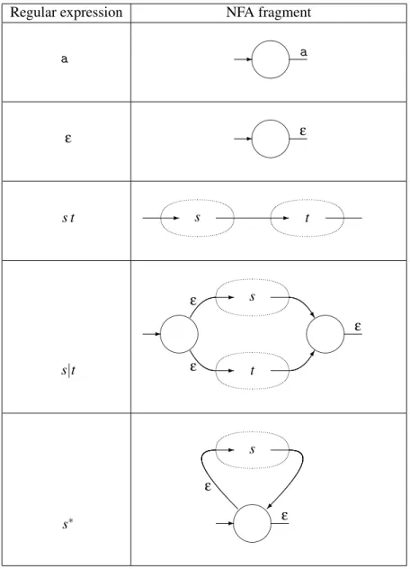
Construction of NFA fragments for regular expressions is shown in figure 2.4. The construction follows the structure of the regular expression by first making NFA fragments for the subexpressions and then joining these to form an NFA frag-ment for the whole regular expression. The NFA fragfrag-ments for the subexpressions are shown as dotted ovals with the incoming half-transition on the left and the out-going half-transition on the right.

When an NFA fragment has been constructed for the whole regular expression, the construction is completed by connecting the outgoing half-transition to an ac-cepting state. The incoming half-transition serves to identify the starting state of

(31)

2.4. CONVERTING A REGULAR EXPRESSION TO AN NFA 19

Regular expression NFA fragment

a

ε

s t - s - t

s|t

-ε

s

t

^

ε

s∗

ε

-ε

s

(32)

1 ε

-ε

2 a

3 c

4 5 -ε -ε 6 R a 7 _b 8 + ε

Figure 2.5: NFA for the regular expression (a|b)∗ac

the completed NFA. Note that even though we allow an NFA to have several ac-cepting states, an NFA constructed using this method will have only one: the one added at the end of the construction.

An NFA constructed this way for the regular expression (a|b)∗acis shown in figure 2.5. We have numbered the states for future reference.

2.4.1 Optimisations

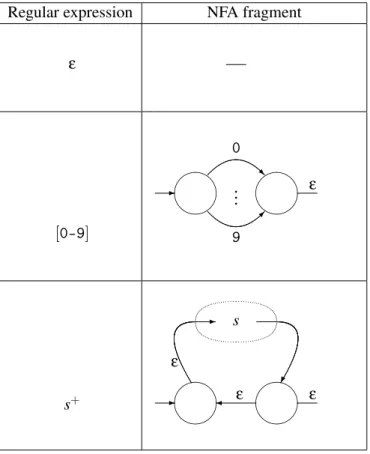
We can use the construction in figure 2.4 for any regular expression by expanding out all shorthand,e.g. convertings+toss∗,[0-9]to0|1|2| · · · |9 ands? tos|ε,etc.

However, this will result in very large NFAs for some expressions, so we use a few optimised constructions for the shorthands. Additionally, we show an alternative construction for the regular expressionε. This construction does not quite follow

the formula used in figure 2.4, as it does not have two half-transitions. Rather, the line-segment notation is intended to indicate that the NFA fragment forεjust

connects the half-transitions of the NFA fragments that it is combined with. In the construction for [0-9], the vertical ellipsis is meant to indicate that there is a transition for each of the digits in [0-9]. This construction generalises in the obvious way to other sets of characters, e.g.,[a-zA-Z0-9]. We have not shown a special construction fors? ass|εwill do fine if we use the optimised construction

forε.

The optimised constructions are shown in figure 2.6. As an example, an NFA for[0-9]+is shown in figure 2.7. Note that while this isoptimised, it is notoptimal. You can make an NFA for this language using only two states.

(33)

2.4. CONVERTING A REGULAR EXPRESSION TO AN NFA 21

Regular expression NFA fragment

ε

[0-9]

_R

0

9

.. .

ε

s+

-ε

ε

ε s

Figure 2.6: Optimised NFA construction for regular expression shorthands

ε

-ε

ε

_R

0

9 .. .

ε

(34)

1 b

-6 a

3

2 3 a

? b

Figure 2.8: Example of a DFA

2.5 Deterministic finite automata

Nondeterministic automata are, as mentioned earlier, not quite as close to “the ma-chine” as we would like. Hence, we now introduce a more restricted form of finite automaton: The deterministic finite automaton, or DFA for short. DFAs are NFAs, but obey a number of additional restrictions:

• There are no epsilon-transitions.

• There may not be two identically labelled transitions out of the same state. This means that we never have a choice of several next-states: The state and the next input symbol uniquely determine the transition (or lack of same). This is why these automata are calleddeterministic. Figure 2.8 shows a DFA equivalent to the NFA in figure 2.3.

The transition relation if a DFA is a (partial) function, and we often write it as such: move(s,c)is the state (if any) that is reached from statesby a transition on the symbolc. If there is no such transition,move(s,c)is undefined.

It is very easy to implement a DFA: A two-dimensional table can be cross-indexed by state and symbol to yield the next state (or an indication that there is no transition), essentially implementing themovefunction by table lookup. Another (one-dimensional) table can indicate which states are accepting.

DFAs have the same expressive power as NFAs: A DFA is a special case of NFA and any NFA can (as we shall shortly see) be converted to an equivalent DFA. However, this comes at a cost: The resulting DFA can be exponentially larger than the NFA (see section 2.10). In practice (i.e., when describing tokens for a program-ming language) the increase in size is usually modest, which is why most lexical analysers are based on DFAs.

(35)

2.6. CONVERTING AN NFA TO A DFA 23

2.6 Converting an NFA to a DFA

As promised, we will show how NFAs can be converted to DFAs such that we, by combining this with the conversion of regular expressions to NFAs shown in section 2.4, can convert any regular expression to a DFA.

The conversion is done by simulating all possible paths in an NFA at once. This means that we operate with sets of NFA states: When we have several choices of a next state, we take all of the choices simultaneously and form a set of the possible next-states. The idea is that such a set of NFA states will become a single DFA state. For any given symbol we form the set of all possible next-states in the NFA, so we get a single transition (labelled by that symbol) going from one set of NFA states to another set. Hence, the transition becomes deterministic in the DFA that is formed from the sets of NFA states.

Epsilon-transitions complicate the construction a bit: Whenever we are in an NFA state we can always choose to follow an epsilon-transition without reading any symbol. Hence, given a symbol, a next-state can be found by either following a transition with that symbol or by first doing any number of epsilon-transitions and then a transition with the symbol. We handle this in the construction by first extending the set of NFA states with those you can reach from these using only epsilon-transitions. Then, for each possible input symbol, we follow transitions with this symbol to form a new set of NFA states. We define theepsilon-closure of a set of states as the set extended with all states that can be reached from these using any number of epsilon-transitions. More formally:

Definition 2.2 Given a set M of NFA states, we defineε-closure(M) to be the least

(in terms of the subset relation) solution to the set equation

ε-closure(M)

=M∪ {t|s∈ε-closure(M) and sεt∈T}

Where T is the set of transitions in the NFA.

We will later on see several examples ofset equations like the one above, so we use some time to discuss how such equations can be solved.

2.6.1 Solving set equations

The following is a very brief description of how to solve set equations like the above. If you find it confusing, you can read appendix A and in particular sec-tion A.4 first.

In general, a set equation over a single set-valued variableX has the form X =F(X)

(36)

whereF is a function from sets to sets. Not all such equations are solvable, so we will restrict ourselves to special cases, which we will describe below. We will use calculation of epsilon-closure as the driving example.

In definition 2.2, ε-closure(M) is the value we have to find, so we make an

equation such that the value ofX that solves the equation will beε-closure(M):

X=M∪ {t|s∈Xandsε_t_∈_T_}

So, if we defineFMto be

FM(X) =M∪ {t|s∈Xandsεt∈T}

then a solution to the equationX=FM(X)will beε-closure(M).

FM has a property that is essential to our solution method: If X ⊆Y then FM(X)⊆FM(Y). We say thatFMismonotonic.

There may be several solutions to the equationX=FM(X). For example, if the NFA has a pair of states that connect to each other by epsilon transitions, adding this pair to a solution that does not already include the pair will create a new solution. The epsilon-closure ofMis theleastsolution to the equation (i.e., the smallestX that satistifes the equation).

When we have an equation of the formX =F(X)andFis monotonic, we can find the least solution to the equation in the following way: We first guess that the solution is the empty set and check to see if we are right: We compare0/withF(0/).

If these are equal, we are done and0/ is the solution. If not, we use the following

properties:

• The least solutionSto the equation satisfiesS=F(S). • 0/⊆Simplies thatF(0/)⊆F(S).

to conclude thatF(0/)⊆S. Hence,F(0/)is a new guess atS. We now form the chain /

0⊆F(0/)⊆F(F(0/))⊆. . .

If at any point an element in the sequence is identical to the previous, we have a fixed-point,i.e., a setSsuch thatS=F(S). This fixed-point of the sequence will be the least (in terms of set inclusion) solution to the equation. This is not difficult to verify, but we will omit the details. Since we are iterating a function until we reach a fixed-point, we call this processfixed-point iteration.

If we are working with sets over a finite domain (e.g., sets of NFA states), wewilleventually reach a fixed-point, as there can be no infinite chain of strictly increasing sets.

(37)

2.6. CONVERTING AN NFA TO A DFA 25 We can use this method for calculating the epsilon-closure of the set{1}with respect to the NFA shown in figure 2.5. Since we want to find ε-closure({1}),

M={1}, soFM=F{1}. We start by guessing the empty set:

F{1}(0/) = {1} ∪ {t|s∈0/andsεt∈T} = {1}

As0/6={1}, we continue.

F{1}({1}) = {1} ∪ {t|s∈ {1}andsεt∈T} = {1} ∪ {2,5} = {1,2,5}

F{1}({1,2,5}) = {1} ∪ {t|s∈ {1,2,5}andsεt∈T} = {1} ∪ {2,5,6,7} = {1,2,5,6,7} F{1}({1,2,5,6,7}) = {1} ∪ {t|s∈ {1,2,5,6,7}andsεt∈T}

= {1} ∪ {2,5,6,7} = {1,2,5,6,7}

We have now reached a fixed-point and found our solution. Hence, we conclude thatε-closure({1}) ={1,2,5,6,7}.

We have done a good deal of repeated calculation in the iteration above: We have calculated the epsilon-transitions from state 1 three times and those from state 2 and 5 twice each. We can make an optimised fixed-point iteration by exploiting that the function is not only monotonic, but alsodistributive:F(X∪Y) =F(X)∪ F(Y). This means that, when we during the iteration add elements to our set, we in the next iteration need only calculateF for the new elements and add the result to the set. In the example above, we get

F{1}(0/) = {1} ∪ {t|s∈0/ andsεt∈T} = {1}

F{1}({1}) = {1} ∪ {t|s∈ {1}andsεt∈T} = {1} ∪ {2,5} = {1,2,5} F{1}({1,2,5}) = F({1})∪F({2,5})

= {1,2,5} ∪({1} ∪ {t|s∈ {2,5}andsε_t_∈_T_}₎

= {1,2,5} ∪({1} ∪ {6,7}) = {1,2,5,6,7} F{1}({1,2,5,6,7}) = F({1,2,5})∪F{1}({6,7})

= {1,2,5,6,7} ∪({1} ∪ {t|s∈ {6,7}andsε_t_∈_T_}₎

(38)

We can use this principle to formulate a work-list algorithmfor finding the least fixed-point for an equation over a distributive functionF. The idea is that we step-by-step build a set that eventually becomes our solution. In the first step we calcu-lateF(0/). The elements in this initial set areunmarked. In each subsequent step,

we take an unmarked elementxfrom the set, mark it and addF({x})(unmarked) to the set. Note that if an element already occurs in the set (marked or not), it is not added again. When, eventually, all elements in the set are marked, we are done.

This is perhaps best illustrated by an example (the same as before). We start by calculatingF{1}(0/) ={1}. The element 1 is unmarked, so we pick this, mark it and

calculateF_{₁_}({1})and add the new elements 2 and 5 to the set. As we continue, we get this sequence of sets:

{1} {

√ 1,2,5} {

√ 1,

√ 2,5} { √ 1, √ 2, √ 5,6,7} { √ 1, √ 2, √ 5, √ 6,7} { √ 1, √ 2, √ 5, √ 6, √ 7}

We will later also need to solvesimultaneous equationsover sets,i.e., several equa-tions over several sets. These can also be solved by fixed-point iteration in the same way as single equations, though the work-list version of the algorithm becomes a bit more complicated.

2.6.2 The subset construction

After this brief detour into the realm of set equations, we are now ready to continue with our construction of DFAs from NFAs. The construction is calledthe subset construction, as each state in the DFA is a subset of the states from the NFA. Algorithm 2.3 (The subset construction) Given an NFA N with states S, starting state s0∈S, accepting states F ⊆S, transitions T and alphabetΣ, we construct an equivalent DFA D with states S0, starting state s0₀, accepting states F0 and a transition function move by:

s0₀ = ε-closure({s0})

move(s0,c) = ε-closure({t|s∈s0 and sct∈T})

S0 = {s0₀} ∪ {move(s0,c)|s0∈S0,c∈Σ}

F0 = {s0∈S0|s0∩F6=0/}

(39)

2.6. CONVERTING AN NFA TO A DFA 27 A little explanation:

• The starting state of the DFA is the epsilon-closure of the set containing just the starting state of the NFA,i.e., the states that are reachable from the starting state by epsilon-transitions.

• A transition in the DFA is done by finding the set of NFA states that comprise the DFA state, following all transitions (on the same symbol) in the NFA from all these NFA states and finally combining the resulting sets of states and closing this under epsilon transitions.

• The setS0 of states in the DFA is the set of DFA states that can be reached froms0₀using themovefunction.S0 is defined as a set equation which can be solved as described in section 2.6.1.

• A state in the DFA is an accepting state if at least one of the NFA states it contains is accepting.

As an example, we will convert the NFA in figure 2.5 to a DFA.

The initial state in the DFA is ε-closure({1}), which we have already

calcu-lated to bes0₀={1,2,5,6,7}. This is now entered into the setS0 of DFA states as unmarked (following the work-list algorithm from section 2.6.1).

We now pick an unmarked element from the uncompletedS0. We have only one choice:s0₀. We now mark this and calculate the transitions for it. We get

move(s0₀,a) = ε-closure({t|s∈ {1,2,5,6,7}andsat∈T}) = ε-closure({3,8})

= {3,8,1,2,5,6,7}

= s0₁

move(s0₀,b) = ε-closure({t|s∈ {1,2,5,6,7}andsbt∈T}) = ε-closure({8})

= {8,1,2,5,6,7}

= s0₂

move(s0₀,c) = ε-closure({t|s∈ {1,2,5,6,7}andsct∈T}) = ε-closure({})

= {}

Note that the empty set of NFA states is not an DFA state, so there will be no transition froms0₀onc.

We now adds0₁ands0₂ to our incompleteS0, which now is{ √

s0₀,s0₁,s0₂}. We now picks0₁, mark it and calculate its transitions:

(40)

move(s0₁,a) = ε-closure({t|s∈ {3,8,1,2,5,6,7}andsat∈T}) = ε-closure({3,8})

= {3,8,1,2,5,6,7}

= s0₁

move(s0₁,b) = ε-closure({t|s∈ {3,8,1,2,5,6,7}andsbt∈T}) = ε-closure({8})

= {8,1,2,5,6,7}

= s0₂

move(s0₁,c) = ε-closure({t|s∈ {3,8,1,2,5,6,7}andsct∈T}) = ε-closure({4})

= {4}

= s0₃

We have seens0₁ands0₂before, so onlys0₃is added:{ √ s0₀,

√

s0₁,s0₂,s0₃}. We next picks0₂:

move(s0₂,a) = ε-closure({t|s∈ {8,1,2,5,6,7}andsat∈T}) = ε-closure({3,8})

= {3,8,1,2,5,6,7}

= s0₁

move(s0₂,b) = ε-closure({t|s∈ {8,1,2,5,6,7}andsbt∈T}) = ε-closure({8})

= {8,1,2,5,6,7}

= s0₂

move(s0₂,c) = ε-closure({t|s∈ {8,1,2,5,6,7}andsct∈T}) = ε-closure({})

= {}

(41)

2.7. SIZE VERSUS SPEED 29

s0₀

* a H H H j b

s0₁ P P P q c U a b

s0₂ a M b

s0₃

Figure 2.9: DFA constructed from the NFA in figure 2.5

move(s0₃,a) = ε-closure({t|s∈ {4}andsat∈T}) = ε-closure({})

= {}

move(s0₃,b) = ε-closure({t|s∈ {4}andsbt∈T}) = ε-closure({})

= {}

move(s0₃,c) = ε-closure({t|s∈ {4}andsct∈T}) = ε-closure({})

= {}

Which now completes the construction ofS0={s0₀,s0₁,s0₂,s0₃}. Onlys0₃contains the accepting NFA state 4, so this is the only accepting state of our DFA. Figure 2.9 shows the completed DFA.

Suggested exercises: 2.2(b), 2.4.

2.7 Size versus speed

In the above example, we get a DFA with 4 states from an NFA with 8 states. However, as the states in the constructed DFA are (nonempty) sets of states from the NFA there may potentially be 2n−1 states in a DFA constructed from ann-state