AN INTERNAL PILOT STUDY WITH INTERIM ANALYSIS
FOR GAUSSIAN LINEAR MODELS
John A. Kairalla
A dissertation submitted to the faculty of the University of North Carolina at Chapel Hill in partial fulfillment of the requirements for the degree of Doctor of Philosophy in the
Department of Biostatistics, School of Public Health.
Chapel Hill 2007
Approved by:
ABSTRACT
JOHN A. KAIRALLA. An Internal Pilot Study with Interim Analysis for Gaussian Linear Models.
(Under the direction of Keith E. Muller and Christopher S. Coffey)
Misspecification of a nuisance parameter can lead to study power far from the desired level. Internal pilots for Gaussian data protect study power by allowing sample size re-estimation based on an interim power analysis using a revised estimate of the variance parameter, but without any data analysis. In order to reduce study time and cost, researchers and sponsors of studies often desire early decision possibilities that the internal pilot design lacks but that group sequential methods allow. Combining early stopping rules with internal pilot methods would increase study flexibility, scope, and efficiency for general linear models.
An internal pilot with an interim analysis (IPIA) design for Gaussian linear models is introduced and defined. The design allows for early stopping for efficacy and futility while also re-estimating sample size needs based on an interim variance estimate. In order for accurate study planning in small samples, exact theory is derived for both the one or two group test setting, as well as more complex multiple degree of freedom hypothesis tests> within the general linear univariate model framework. Exact and computable forms of distributions allow accurate calculations of power, type I error rate, and expected sample size.
ACKNOWLEDGEMENTS
I wish to thank my dissertation chairmen Keith Muller and Chris Coffey for all of their support and encouragement during the course of this research. Their active interest allowed this work to prosper despite often many miles of separation. I am very grateful to have had the opportunity to work closely and learn from both of you (including the late night theory sessions that went on long past Keith's bedtime). I would also like to thank my committee members Lisa LaVange, Todd Schwartz, and Annelies Van Rie. In addition to their
unwavering support and flexibility, they each provided valuable insight and context for this work that will no doubt help my career progress. I truly hope to continue working with each of them in the years ahead.
I would also like to thank the UNC Department of Biostatistics for all of the support I have received. First, Craig Turnbull introduced me to the field as an undergraduate and prepared me for graduate research as adviser of my honor's thesis. Second, I am very grateful to NIH grant funding I have received with PIs: Ed Davis, Lloyd Edwards, Larry Kupper, and Amy Herring. Also, my GRAs with Richard Henderson and Keith Muller were incredibly valuable experiences in consulting, programming, organizing, and document preparation as well as financially supportive. Finally, the staff and students in biostatistics have been wonderful to be around and are indispensable to my graduate education.
I also need to thank my wife Ashey for her love and support. She has been so
TABLE OF CONTENTS
LIST OF TABLES... ix
LIST OF ABBREVIATIONS... xi
Chapter 1. INTRODUCTION AND LITERATURE REVIEW... 1
1.1 INTRODUCTION...1
1.2 LITERATURE REVIEW... 3
1.2.1 Introduction... 3
1.2.2 Group Sequential Methods...4
1.2.3 Stochastic Curtailment...8
1.2.4 Sample Size Re-Estimation... 10
1.2.4.1 Introduction... 10
1.2.4.2 Flexible Designs... 11
1.2.4.3 Adaptive Designs...11
1.2.4.4 Sample Size Re-Estimations Based on Conditional Power...13
1.2.4.5 Internal Pilot Designs... 14
1.2.4.6 Review of Related Topics...17
1.3 SUMMARY...21
2. INTERNAL PILOT WITH INTERIM ANALYSIS FOR SINGLE DEGREE OF FREEDOM HYPOTHESIS TESTS...22
2.1 INTRODUCTION... 22
2.2 THE IPIA MODEL AND PROPERTIES... 27
2.2.1 Notation... 27 2.2.2 The IPIA Model...28
2.2.3 IPIA Properties... 32
2.3 THE IPIA PROCEDURE AND PROPERTIES...40
2.4 KEY ANALYTIC RESULTS FOR PROCEDURE...43
2.5 EXAMPLES... 46
2.5.1 Motivation for Examples...46
2.5.2 Computational Methods... 48
2.5.3 Example 2.1 Results... 50
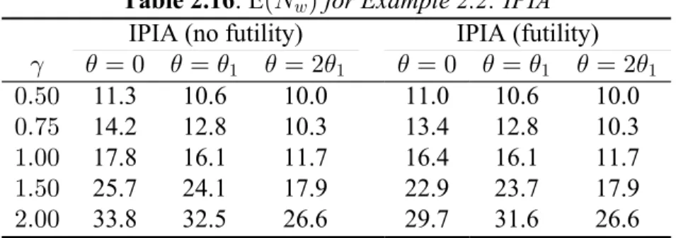
2.5.4 Example 2.2 Results... 54
2.6 DISCUSSION...58
3. PLANNING PROCEDURES FOR AN INTERNAL PILOT WITH INTERIM ANALYSIS DESIGN... 62
3.1 INTRODUCTION... 62
3.1.1 Motivation... 62
3.1.2 Literature Review... 63
3.2 THE IPIA MODEL AND PROCEDURE... 65
3.2.1 Notation... 65 3.2.2 The IPIA Model...66
3.2.3 The General Procedure... 68
3.3 CRITICAL VALUE SELECTION...68
3.3.1 Overview... 68
3.3.2 Distributional Assumptions... 69
3.3.3 The IPIA Bounding Method...70
3.4.2 Interim Sample Size Selection...73
3.5 EXAMPLES... 74
3.5.1 Example Motivation... 74
3.5.2 Example Methods... 74
3.5.3 Computational Methods... 75
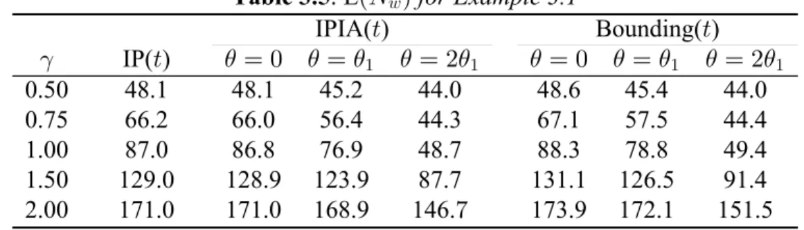
3.5.4 Example 3.1 Results... 76
3.5.5 Example 3.2 Results... 79
3.5.6 Interim Sample Size Selection Results...81
3.6 DISCUSSION...83
4. INTERNAL PILOT WITH INTERIM ANALYSIS FOR MULTIPLE DEGREE OF FREEDOM HYPOTHESIS TESTS...87
4.1 INTRODUCTION... 87
4.1.1 Motivation... 87
4.1.2 Literature Review... 88
4.2 THE IPIA MODEL AND PROPERTIES... 89
4.2.1 Notation... 89 4.2.2 The IPIA Model...90
4.2.3 IPIA Properties... 92
4.3 THE IPIA PROCEDURE AND PROPERTIES... 101
4.4 KEY ANALYTIC RESULTS FOR PROCEDURE... 104
4.5 AN EXAMPLE...107
4.5.1 Motivation for the Example...107
4.5.2 Computational Methods...110
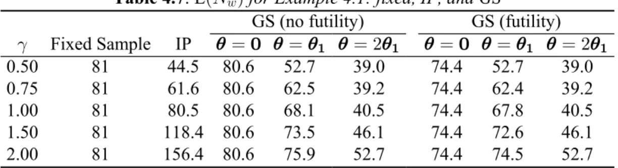
4.5.3 Example 4.1 Results...111
5.1.1 Chapter 2: Internal Pilot with Interim Analysis for
Single Degree of Freedom Hypothesis Tests...119
5.1.2 Chapter 3: Planning Procedures for an Internal Pilot with Interim Analysis Design... 119
5.1.3 Chapter 4: Internal Pilot with Interim Analysis for Multiple Degree of Freedom Hypothesis Tests... 120
5.2 FUTURE RESEARCH... 121
5.2.1 Futility Bounds... 121
5.2.2 Sample Size Re-Estimation Method... 121
5.2.3 Selection of Interim Sample Size...122
5.2.4 Computation...123
5.2.5 Strategies for Multiple Degree of Freedom Tests...123
5.2.6 Generalizations to Other Settings... 124
APPENDIX A: CHAPTER 2 PROOFS...126
APPENDIX B: CHAPTER 4 PROOFS...133
LIST OF TABLES
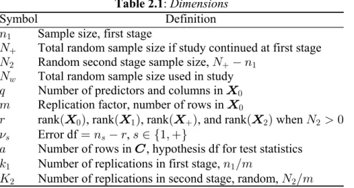
Table2.1 Dimensions... 31
2.2 Parameters and constants...31
2.3 Internal pilot with interim analysis notation...32
2.4 General procedure... 40
2.5 Two-stage designs... 47
2.6 Simulation and calculation times (minutes)... 49
2.7 Design parameters for Example 2.1... 50
2.8 Type I error rates‚100 for Example 2.1...50
2.9 Power‚100 for Example 2.1... 51
2.10 E RA for Example 2.1: fixed, IP, and GS...52
2.11 E RA for Example 2.1: IPIA... 53
2.12 Design Parameters for Example 2.2... 54
2.13 Type I error rates‚100 for Example 2.2...55
2.14 Power‚100 for Example 2.2... 56
2.15 E RA for Example 2.2: fixed, IP, and GS...57
2.16 E RA for Example 2.2: IPIA... 57
3.1 General Procedure... 68
3.2 Design parameters for Example 3.1... 76
3.3 Type I error rates‚100 for Example 3.1...76
3.4 Power‚100 for Example 3.1... 77
3.5 E RA for Example 3.1... 78
3.6 Design parameters for Example 3.2... 79
3.7 Type I error rates‚100 for Example 3.2...79
3.10 Type I error rates‚100 for 1−e0.25, 0.5, 0.75 ... 81f 3.11 Power‚100 for 1 −e0.25, 0.5, 0.75 ... 82f 3.12 E RA for 1 −e0.25, 0.5, 0.75 ... 83f
4.1 General procedure...101
4.2 Two-stage design... 108
4.3 Simulation and calculation times (hours) for Ex. 4.1... 111
4.4 Design parameters for Example 4.1...112
4.5 Type I error rates‚100 for Example 4.1...112
4.6 Power‚100 for Example 4.1...113
4.7 E RA for Example 4.1: fixed, IP, and GS...113
LIST OF ABBREVIATIONS
AD Adaptive designCP Conditional power
GLUM General linear univariate model GSM Group sequential method IP Internal pilot
CHAPTER 1. INTRODUCTION AND LITERATURE
REVIEW
1.1 INTRODUCTION
An important aspect to consider during study planning is an appropriate sample size to detect an effect of interest for given type I error rate and power. Power in studies often depends on one or more unknown nuisance parameters. For example, in a one group -test,> let \ \ á", #, be independent Gaussian observations with mean and unknown error) variance . The goal is to test 5# L À! ) œ ! versus L À" ) Á ! with type I error rate andα> power at T> )œ )". The required sample size for the test with given , , and dependsα> T> )" on . In practice, sample size needs are usually calculated using an estimated value, ,5# 5!# taken from similar studies or earlier trials. This value, however, is often not appropriate due to characteristics such as differing populations or inadequate sample size of test trials. Study power for a Gaussian linear model is very sensitive to misspecification of the variance parameter, .5#
In general, sample size re-estimation techniques have been developed as tools for adjusting the size of a study to meet its planned objectives. To ensure a correctly planned study, very few interim analyses are conducted. In fact, two-stage designs have become popular due to their practicality, effectiveness, and lack of administrative burden (Shih, 2006). Specifically, internal pilot (IP) designs are two-stage designs that allow sample size modification based on revised estimates of nuisance parameters without interim data
and Muller (1999) derived the exact distribution of the IP test statistic in a computable form. The theory includes -tests as special cases and allows for flexibility of hypotheses. The> exact theory also made study planning possible for small sample designs.
Researchers and sponsors of clinical trials and other studies would also like the ability to reach early decisions when hypothesis outcomes are clear. Early decisions to stop a trials may allow more effective treatments to reach a target population quickly and can protect patients from ineffective, inefficient, or harmful treatments. Stopping early can also allow resources to be diverted to other promising research, boosting overall research efficiency. To address the need for early stopping capability in study design, study monitoring procedures such as group sequential and stochastic curtailment methods have been developed.
Combining IP designs with early stopping rules would increase study flexibility, scope, and efficiency for general linear models. In this dissertation, the exact distributions
necessary for small sample internal pilots with an interim analysis at the IP stage for GLUMs with fixed effects and Gaussian errors are derived. The study design is hence referred to as the internal pilot with interim analysis (IPIA) design. In Chapter 2 of this dissertation, the model is introduced, the procedure is explained, and the necessary distributions for the IPIA design for single degree of freedom tests are derived. These study designs consist of one and two group comparisons with unknown, common variances for -tests as well as other study> designs. The necessary distributions include a computable form of the exact joint
distribution of the first and second stage test statistics conditional on a final sample size. Knowledge of these forms then allow for derivation of exact forms for unconditional study power, type I error rate, and expected sample size. Examples will portray the characteristics of the IPIA design and compare them with some other common designs.
expected sample size for a design, these factors must be pre-specified. In Chapter 3 of this dissertation, I discuss and evaluate procedures for planning the studies described in Chapter 2. The goal is to achieve sound study design strategies that control the type I error rate while best maintaining the power and sample size advantages of the IPIA designs.
In Chapter 4, the results necessary for the IPIA design for multiple degree of freedom tests in the GLUM framework are derived. These tests consist of more complex hypotheses such as multiple group comparisons. The key new result is the exact conditional joint distribution of the first and second stage test statistics. The new exact distributions may be used to solve for power, type I error rate, and expected sample size in these study designs. An example will demonstrate the characteristics of the IPIA design in this more complex setting.
1.2 LITERATURE REVIEW
1.2.1 Introduction
Interim analysis (or interim monitoring) often takes place during the course of clinical trials to acquire knowledge to make decisions such as design modification or early stopping. Jennison and Turnbull (2000, Chapter 1) categorized reasons for conducting interim analyses into three loosely defined classes: ethical economic, , andadministrative. One ethical
consideration includes ensuring that patients are not exposed to unsafe, inferior, or
ineffective treatments. Another ethical consideration is the need to reallocate resources to other promising treatments when a current study is unlikely to show a benefit. Economic reasons for conducting interim analyses also exist from the ability to stop a trial early. If a trial stops early with a positive result, a treatment can reach the public more quickly, saving time and resources as well as generating an expedited revenue source for sponsors.
Administrative reasons for conducting interim analyses include determining if the
experiment is following both the designed protocol and planned assumptions. Assumptions made during sample size planning often include values for outcome variability in quantitative data or incidence rate values for binary data.
Three main types of interim analysis are group sequential methods, stochastic
curtailment, and sample size re-estimation. Group sequential methods are analyses in which groups of subjects are enrolled and analyzed sequentially. They are designed to shorten the expected length of a study by allowing early hypothesis decisions to be reached if true effect sizes are larger or smaller than anticipated. Stochastic curtailment is another method of shortening a study based on calculating probabilities of achieving hypothesis decisions conditional on accumulated observed data. Sample size re-estimation procedures cover a wide range of possible study designs. All include possible adjustment to the planned sample size of a study (increases and/or decreases) in light of new information concerning aspects of the study.
Specific to sample size re-estimation, methods vary based on what information may be used, when the information is used, and the decisions made as a result. Flexible designs allow the most freedom with few restrictions if the type I error rate is controlled. Adaptive designs restrict the study to pre-planned design modifications based only on information internal to the study. Internal pilot designs allow for modification of a study based only on re-estimation of nuisance parameters, such as the error variance for Gaussian outcomes. The sample size re-estimation methods also vary based on if rules are included for early stopping at interim stages.
1.2.2 Group Sequential Methods
research focus has been the use of GSMs in clinical trials. An important reason for this focus is to stop randomization of patients to a potentially inferior treatment when a significant treatment difference can be proven with high probability.
An early influence in sequential analysis was Wald's (1947) sequential probability ratio test (SPRT). The SPRT tests between two simple hypotheses by sampling observations while the likelihood ratio remains in an interval Ð+ß ,Ñ for constants , chosen to+ ,
approximately control type I and type II error rates. Armitage (1975) developed methods for fully sequential analysis in medical studies. In these methods, data must be enrolled in matched pairs and accumulating data monitored continuously. However, this was not proven to conform well and did not achieve widespread use. GSMs worked better within clinical trials settings and became a popular alternative with the release of papers by Pocock (1977) and by O'Brien and Fleming (1979). For normally distributed data with known variance, these papers presented clear approaches for two-sided group sequential testing that controls the type I error rate while maintaining power. In a basic group sequential design for a comparison of two treatments, a maximum number of stages ( ), group-size ( ), and critical5 7 values for each stage ( for -3 3 − "ß á ß 5e f) are pre-determined. Subjects are randomized to treatment with the constraint that for each stage, subjects are assigned to each treatment.7 For stage a standardized statistic, , is computed using data from the first groups and the3 ^3 3 study stops with rejection of the null hypothesis, L0, if k k^ -3 3, and continues otherwise. At stage 5ß L! is accepted if k k^5 -5.
Critical values are chosen to preserve the overall type I error rate ( ), i.e.,α
(3 5) if k k^ $3 and then uses the ordinary stopping bound at the final stage. The final stage could also be slightly modified to accurately control type I error rate. This method has gained traction when trial planners need a simple rule to stop a study only when a clear and strong effect is observed while paying little penalty in the final critical value. Due to multiple testing possibilities, the maximum sample size of #57 is determined by a
procedure-specific inflation factor multiplied by the sample size from a corresponding fixed sample test.
Wang and Tsiatis (1987) described a family of two-sided test designs, indexed by a parameter (? ! Ÿ?Ÿ !Þ&), for use in the general GSM framework. The family generalizes the Pocock and O'Brien-Fleming methods with ?œ ! giving the O'Brien-Fleming test and ?œ0.5 giving the Pocock test. The adjusted critical values depend on , , and ; the5 α ? maximum sample size inflation factors depend on , , and where represents the5 α ", ? " target type II error rate. Lan and DeMets (1983) introduced a flexible way to construct boundaries in group sequential methods using an -spending function. The idea is to defineα a monotonely increasing function for the information fraction > Ð! Ÿ > Ÿ "Ñ: α > with α ! œ ! and α " œα, the desired type I error rate. This function characterizes the rate at which the error level is spent. This method can approximately emulate the Pocock andα O'Brien-Fleming boundaries, but allows for other methods, for variable timing, and number of analyses. A number of possible error spending functions have been proposed in the literature (Lan and DeMets, 1983; Hwang et al., 1990; Kim and DeMets, 1987; Jennison and Turnbull, 1989).
significant study is low. Gould (1983) proposed methods for early stopping only to accept the null if a test has a -value greater than a fixed critical value. Pampallona and Tsiatis: (1994) described a one parameter ( ) class of boundaries for group sequential methods? based on the family introduced by Wang and Tsiatis (1987) that can be used for any type I and type II error rate choices. Whitehead and Straton (1983) and Whitehead (1997) described an alternate method known as the triangular test based on combining two one-sided tests. Jennison and Turnbull (2000, Chapter 5) compared these methods as well as providing some tables of constants. Since allowing the study to stop to accept L! for small effect sizes may have significant savings in time and cost, Jennison and Turnbull (2000, Chapter 5) recommend that the stopping bounds be considered in all group sequential two-sided tests. Lachin (2005) explored the use of futility monitoring plans based on conditional power within group sequential testing. The method has a single futility analysis at a
specified information fraction (such as X œ !Þ&) amidst the other interim tests before, at, and after the futility analysis. Using O'Brien-Fleming bounds, the plan approximately controls the type I error rate and maintains power while adding sample size benefits under the null. Spurrier (1982) presented two-stage tests of hypothesis in the general linear univariate model with normally distributed and independent errors, a special case of group sequential methods. He proposes an ad hoc sample size selection method with each stage being of size !Þ' 8* where is the sample size of a fixed sample test. In the method, the first sample! 8! leads only to decisions to stop for efficacy (if J -" ?, reject L Ñ! or futility (if J Ÿ -" 6, accept L!), or to take the final sample (if - J - Ñ6 " ? . The null hypothesis is then either accepted or rejected if the final test statistic, J, is below or above critical value ,-+
compromise between fixed sample and sequential methods with more stages, offering well defined theory with a reduction in expected sample size while minimizing uncertainty of sample size and duration of study.
While most group sequential methods rely on large sample critical values or known variances, some alternative critical value selection methods have been proposed and
reviewed. One simple approach suggested by Pocock (1977) shown to work quite well when variance is unknown is to take the significance level of Gaussian derived critical values and use them along with sample size to calculate corresponding distributed critical values.> Since the distribution takes into account the sample size used for estimation in the form of> degrees of freedom, it better relates to the uncertainty of the variance estimate used in the test statistic. Although the statistics are sequences and hence have a joint relationship, this simple method approximately controls the type I error rate for group sequential designs. Additionally, Shao and Feng (2007) described a Monte Carlo method for calculation of critical values in a small sample group sequential studies. Through simulation they showed that their method works well at controlling the type I error rate and maintaining power with an expected increase in expected sample size.
Group sequential methods have also been further generalized in various ways. Jennison and Turnbull (1991, 1997) described distributional theory for group sequential , , and > ;# J tests. Methods have also been described to allow for flexibility in the number, timings, and sizes of looks (Jennison and Turnbull, 2001).
1.2.3 Stochastic Curtailment
stopped, however, if the outcome while not inevitable, is highly probable. This can increase the efficiency of a study by decreasing expected sample size.
One approach to stochastic curtailment is the conditional power (CP) approach. CP is defined here as the probability of a statistically significant result (rejecting L!) at the end of a study given a true value of the effect size and conditional on data already observed. Let T3 ) be the CP at some stage for effect . A method described by Lan et al. (1982) defines3 ) a formal stopping rule where L0 is rejected if T3 )! -ß for a constant such as - !Þ) or !Þ*. The logic behind this method is that the test will not likely accept the null at this point even if it is true. Alternatively, a test could be stopped for futility (accept L!) if " T3 )" -w where is an alternative of interest. Proschan et al. (2006, Chapter 3) noted that, under a)" futility scenario, as estimate of nuisance parameters such as the sample variance could be used to recalculate unconditional power of the study. A low value implies an uninformative acceptance of L! and is further evidence to curtail the study. Under the scenario of a low CP and a high unconditional power, continuing the study may be useful to clearly differentiate between the hypotheses. A criticism of the CP stopping methods (Jennison and Turnbull, 2000, Chapter 10; Dmitrienko and Wang, 2006) is that they are based on calculations under only specific values of and ignore information about the effect size from current data. For) example, an overly optimistic value of would make a study difficult to stop for futility)" despite unpromising results.
Another form of stochastic curtailment known as the predictive power (PP) method utilizes a mixture of Bayesian and frequentist ideas. Jennison and Turnbull (2000, Chapter 10) described the approach, which averages conditional power over values of effect with) weighting corresponding to current belief: a posterior distribution given the prior distribution and the observed data. This method gives an informative probability of success or failure in a study and, like the CP method, formal rules can be developed for early stopping for
(1986) for binary endpoints. Choi and Pepple (1989) applied the Bayesian-frequentist approach to normally distributed data. Jennison and Turnbull (2000, Chapter 10) and Bernardo and Ibrahim (2000) also discussed the mixture approach in general settings. Criticisms of the method include the lack of a clear frequentist interpretation and that it is inconsistent with Bayesian principles (Jennison and Turnbull, 1990, Chapter 10).
A third method, described by Dmitrienko and Wang (2006), introduces a family of Bayesian stopping bounds by extending a Bayesian predictive method proposed by Geisser (1992). The paper reviews and compares the methods for stochastic curtailment. Dmitrienko et al. shows that the Bayesian and Bayesian-frequentist methods typically allow higher probability of early stopping with the pure Bayesian method being more sensitive to the choice of prior distribution. Dmitrienko et al. (2005, Chapter 4) provided SAS macros for the computation of stochastic curtailment stopping bounds for the three methods.
1.2.4 Sample Size Re-Estimation
1.2.4.1 Introduction
Sample size re-estimation (SSR) procedures differ from traditional and classical group sequential methods. This difference occurs as at least some of the information accrued during a study (possibly external to the study) is used to determine the size of future
event rates have led to researchers desiring the ability to make midcourse adjustments to the sample size of the study.
SSR methods vary by the number of stages used, the allowance for early stopping for efficacy and/or futility, the information used for re-estimation, if the adaptation protocol must be pre-specified, and if sample sizes are allowed to decrease. The great volume of recent research and sometimes lack of clear definitions and delineations has led to a confusion in terminology for similar methods. Different types of SSR methods will be introduced in this section with a focus of clarifying the similarities and differences that exist between them.
1.2.4.2 Flexible Designs
Flexible designs are study designs that permit mid-trial modifications with very little
restriction. Information for study modifications can come from information internal or external to the trial. Also, adaptation does not need pre-specification. However, a major design consideration for flexible designs is to maintain the type I error rate in order to better maintain study validity. Flexible designs specifically will not be covered here; instead a meaningful subset will be discussed: adaptive designs.
1.2.4.3 Adaptive Designs
Recently, there has been great interest in the development of adaptive design (AD) methodology. ADs for clinical trials offer researchers flexibility to redesign trial procedures and analysis at interim stages. Current research, however, has created a confusion in
when referring to ADs here. Under this definition, the adaptations only use information from accumulating data internal to the trial as opposed to flexible designs which can also
incorporate external information. The PhRMA working group also stresses that the changes should be made "by design" and not undertaken on an ad hoc basis. The definition makes it clear that adaptive designs are not meant to be a remedy for poor planning. Rather, ADs are meant to be designed study enhancements aimed at maintaining study validity and integrity while increasing efficiency of drug development and utilization of resources.
Bauer and Köhne (1994) and Proschan and Hunsberger (1995) were two of the early papers describing AD methods for adapting studies while maintaining type I error rate controls. Bauer and Köhne used a weighted Fisher's combination test for a two-stage one-sided test with possible early stopping and SSR based on effect size. Alternatively, Proschan and Hunsberger based their test on a conditional error approach: overall type I error rate is controlled as long as a second stage test conditional on the first stage results maintains the type I error rate. Wassmer (1998) showed that for two stages and one sided hypotheses, the methods of Bauer and Köhne (1994) and Proschan and Hunsberger (1995) are extremely similar in power and expected sample size. Other related adaptive methods include the methods described by Lehmacher and Wassmer (1999) and Cui et al. (1999). Both
approaches use classical group sequential stopping boundaries with updating of sample size based on data observed in a first study and use fixed, predetermined weights to combine stage-wise results. The Lehmacher and Wassmer approach combines -values using the: inverse normal approach with fixed, predetermined weights (usually equal across stages). All of the methods above assume the variance is known for the study.
A number of issues have been raised concerning the use of adaptive designs. An
of a positive effect for a negative estimate (Proschan and Hunsberger, 1995; Burman and Sonesson, 2006). The weighting schemes used to protect type I error rate also violate basic sufficiency principles since observations from different stages are given different weightings (Jennison and Turnbull, 2003). Tsiatis and Mehta (2003) and Jennison and Turnbull (2006) argued that while adaptive designs have a place for preserving a study if unplanned analyses are conducted, group sequential methods offer more efficiency under reasonable conditions.
1.2.4.4 Sample Size Re-Estimation Based on Conditional Power
Conditional power (CP) has been proposed as a tool for the recalculation of sample size in clinical trials for adjusting study power (Proschan and Hunsberger, 1995). Two ways exist using interim data to calculate a probability of rejection in the trial given the results observed thus far. The first type of probability calculation assumes the true effect size, , is equal to) the value the study was originally powered to detect, . The other type assumes the true)" effect size is the observed estimateßs)3, for an interim stage .3
The logic supporting the SSR is the adjustment of the sample size to that needed to maintain study power at the target rate. Often, this kind of calculation includes the revised estimates of nuisance parameters for SSR purposes (Denne, 2001). In this sense, the SSR is similar to an internal pilot technique. The difference lies in that regardless if or is)" s)3 assumed to be the true effect in the calculations, the calculations depend on the observed value of the test statistic at the interim stage. While different conceptually, both kinds of CP calculations raise questions in this context.
However, many researchers and even sponsors might prefer to keep the positive interim stage data and increase their overall probability of success in the trial.
If instead the study is re-powered to achieve target power at ) œ s)3 (Cui et al., 1999), more issues are raised. In this case, the study is repowered at a new hypothesis of ) œ s)3. If the sample size is increased, then statistically, the effect of interest is decreased. Uses for the procedure such as flexibility to external factors and cases where an effect of interest is unclear have been described by various researchers. In the case where sample size is decreased due to interim analysis, the test could be underpowered to detect the originally planned effect size if it is in fact true.
1.2.4.5 Internal Pilot Designs
A poor variance value used in sample size calculations can greatly impact the power of a clinical trial. A value that is too low leads to an underpowered study with a small chance of success regardless of the treatment's efficacy. Alternatively, a value that is too large leads to a waste of money and other resources in an overpowered trial. Stein (1945) introduced a two-stage -test design with power independent from the variance. This technique updates> the sample size at an interim stage using only the observed sample variance. The final test statistic uses information from all subjects for treatment effect, but only the variance estimate from the first sample. For a two group comparison, the final test statistic under the null hypothesis follows a distribution with > 8 #" degrees of freedom where is the total8" sample size at the interim stage. A criticism of the method is that it throws away information about the variance from the second sample. Proschan and Wittes (2000) noted that the technique is not robust to possible changes in variance during the course of the trial. Also, Coffey and Muller (1999) showed Stein's method does not perform well when the second sample is large compared to the first.
Stein's method by using the pooled variance from all subjects in the final test statistic and treating the final sample size as if it were fixed. Simulation was used to show power and type I error rate for this test for an example using a preplanned sample size of and an)' internal pilot using half of the preplanned sample. For large samples and an
upward-restricted sample size adjustment design, they concluded that the type I error rate and power were well preserved.
Birkett and Day (1994) explored the use of different sizes for the interim stage rather than half of the initial fixed sample estimate. This design also allowed for decreases in the final sample size. The conclusion was reached that as long as there are enough degrees of freedom (µ #!) in the IP stage, the type I error rate and power are close to target levels. Coffey and Muller (1999) showed by counterexample that significant type I error rate inflation (up to 14% in their example) can still occur in test studies under this scenario. Coffey and Muller determined that the choice of internal pilot size and other design parameters can strongly affect results and should be inspected during planning for specific studies. Despite the potential benefits in power properties or sample size savings, the risk of type I error rate inflation, caused by a downward biased variance estimate (Proschan and Wittes, 2000; Miller, 2005) offsets the benefits in the minds of many researchers (Kieser and Friede, 2000) and regulatory agencies (ICH Topic E9 Guideline, Section 4.4). This risk has led many researchers to propose methods to control the type I error rate. These methods can be separated by if blinding is maintained on treatment allocation at the interim analysis, and by if the test statistic or critical value is modified to preserve the type I error rate.
approximately controls the type I error rate when the true treatment difference is close to the prespecified difference. A disadvantage of the blinded methods is that the one-sample variance changes in relation to the treatment effect, which could cause inflation of sample sizes if the treatment effect is larger than thought. Friede and Kieser (2001) note that the sample size inflation is small when the true effect is close to the prespecified effect.
Many methods to control the type I error rate with unblinding have been proposed. Miller (2005) points out that the decision on whether or not to use blinded procedures should be made on a case-by-case basis and notes that careful control of information and the use of an independent statistician can mitigate potential biases. Stein's method controls the type I error rate by only using information from the first sample for the variance estimate. Zucker et al. (1999) proposed an alternate method where only the information about the variance independent from the IP stage is used in the final test statistic. This method controls the type I error rate both conditionally and unconditionally. Denne and Jennison (1999) proposed a method based on Stein's test that uses all information about the variance, but includes a degree of freedom adjustment to the final test statistic that does not guarantee bounding of type I error rate, but appears to work well in general. Proschan and Wittes (2000) introduced a method that uses an unbiased variance estimate by fixing weights between the IP stage and the second stage portions of the final variance estimate. Coffey and Muller (2001)
introduced a bounding method which alters the critical value so that the maximum type I error rate inflation is equal to the target rate. The method by Miller (2005) adjusts the normal variance estimate to control the type I error rate.
The researchers also derived computable forms for the exact distribution for the test statistic, which includes -tests as special cases. Kairalla et al. (2007) released a free software>
package based in SAS/IML®ÐSAS Instituteß #!! Ñ4 for exact power, type I error rate, and expected sample size calculations for a wide range of internal plot designs. For binary outcomes, Proschan (2005) describes the possibility of an underpowered study if the control event rate is overestimated. The paper describes two methods for re-estimating the sample size, both with asymptotic validity. In an unblinded method, the control event rate can be re-estimated and used for SSR. Alternatively, Gould (1992) described a blinded SSR procedure for binary data based on the overall event proportion. Internal pilot methods have also been extended into other settings of interest including ordinal data (Bolland et al., 1998), time-to-event data (Whitehead et al, 2001), and repeated measures (Shih and Gould, 1995; Lake et al., 2002; Zucker and Denne, 2002; Coffey and Muller, 2003).
1.2.4.6 Review of Related Topics
For clinical trials with Gaussian outcomes, IP designs allow for an update to sample size based on an error variance estimate taken at an internal stage. While studies may be
lengthened or shortened by this estimate, the main objective is to ensure that the study is sufficiently powered to detect an effect size of interest. Group sequential methods, on the other hand, are designed to allow for a reduction in sample size if effect sizes deviate substantially from anticipated sizes. A successful combination of GSMs with IP based sample size re-estimation would allow for early stopping due to effect size differences and also help assure correctly powered studies for an effect of interest with respect to the true variance, a nuisance parameter. There have been a number of papers considering procedures for combining GSM and IP studies to obtain their respective benefits.
variance using a single sample estimate. Arghami and Billard (1992) defined a partial sequential procedure also based on the SPRT and a Stein-like variance estimate. Hochberg and Marcus (1983) described a three-stage test for a one-sided, two-group comparison. This comparison uses variance information from a first sample to determine sample sizes for two testing stages. All of these procedures share the disadvantage of only incorporating early stage variance information into the test statistics.
Facey (1992) described a Phase 2 trial design using the triangular test stopping bounds. She compared the use of powering to absolute or standardized treatment differences. Type I error rate inflation was high for the absolute differences and more reasonable for the
standardized differences in the cases considered (max type I error rate of !Þ!&* for target !Þ!&). Gould and Shih (1998) used a blinded variance estimate from the initial stage to fix future sample sizes. The procedure only allows for sample size increases to the group sequential procedure if the variance estimate is at least a constant factor larger than the planning value (increase sample size if 5s "# -5!# with - œ "Þ$$, for example). A few methods are explored, such as redistributing the sample sizes to match the originally planned information times, or allowing the sample sizes to vary in pre-planned or unplanned manners. They concluded through simulation, with a small fraction of error dedicated to the first testing stage, that the procedure works adequately with two testing stages. Whitehead et al. (2001) explored through simulation a method similar to Gould (1998) for comparing effects from two groups by updating estimates of the standardized difference, $ 5"Î #, where is the$" effect of interest and the common variance. The study is first planned to detect5#
sample scenario was 8 œ *#). Despite the large samples, type I error rate inflation occurred in simulations they ran with or without SSR (up to !Þ!$# for target of !Þ!#&). The authors noted that a large problem is that asymptotic results underlying sequential theory only become accurate for very large samples.
Denne and Jennison (2000) proposed a group sequential -test with sample size update.> This was based on the variance for a two-sided single group test of mean with early stopping to reject the null. A test based only on a Stein-like first variance estimate was first described. This method was used as a stepping stone to define a test procedure where the maximum sample size is recalculated at each stage with updated variance estimates. The remaining sample is then split based on the number pre-planned number of testing stages. Testing is not done at the first stage if the originally planned first stage testing fraction is not met. Thus, a two testing stage procedure could have three or more stages in total. In the
calculations for critical values and sample size adjustments, both a type I error rate spending function and a degree of freedom correction are used to reflect the uncertainty of the variance estimates. The "effective" number of degrees of freedom at stage is defined to be3
8 " % 8 83 " " for ! Ÿ Ÿ "% and the first stage sample size. Based on calculations8" for several examples, % œ "Î% is recommended to approximately achieve target error rates. For tests with two and five stages, Denne and Jennison showed by a combination of
design using updated variance estimates at each stage has better power and sample size properties.
Another approach to clinical trial monitoring with nuisance parameter based sample size adjustment is the information based approach described by Mehta and Tsiatis (2001) or Tsiatis (2006). Since statistical precision is determined by the amount of statistical
information, a study should continue until the needed statistical information level is reached. At this point the study will closely achieve the desired statistical power. Mehta and Tsiatis described the method for use within group sequential designs that allow for early stopping while updating the estimated maximum sample size at each analysis stage as nuisance parameter estimates are updated. Group sequential stopping bounds along with an inflation factor on needed information (and hence needed sample size) due to multiple testing were advocated. They used standardized test statistics with critical boundary determination based on the error spending technique used. Large samples are needed for this design in order to avoid type I error rate inflation caused by asymptotic properties in the distribution of the test statistics and boundary point calculations as well as from the of a downwardly biased
variance estimate in study stages following the first. This is the same cause of type I error rate inflation found in unadjusted internal pilot studies; see Proschan and Wittes (2000) or Miller (2005)for details.
Most work has dealt only with the one or two group -test scenario. This work> represents an intersection with the topics of this dissertation. Many of the results promote general techniques for group sequential designs and are typically based on underlying large sample assumptions to account for designs adjustments made in the trials. Group sequential designs typically have a primary goal of reducing average sample size by frequently
sample size reductions are a secondary benefit. The primary focus of this dissertation is maintaining power by updating sample size needs, while incorporating the benefits of group sequential theory by allowing the possibility of early stopping at the interim stage.
1.3 SUMMARY
Many prospective research studies and even clinical trials are not large enough for asymptotic properties to hold. Researchers in small sample continuous outcome settings need the ability to control type I error rate and maintain power over possible values of the error variance, a nuisance parameter, while minimizing sample size needs. These small sample settings can be one or two group studies ( -tests), multiple group comparisons, or> other designs. Distributional knowledge and effective protocols in these settings would be valuable to study designers.
Currently methods do not exist for exact theory calculations of power, type I error rate, and expected sample size in small samples for an internal pilot design with interim analysis for early stopping. These calculations could greatly increase the efficiency of study planning through fast direct calculation. Useful and accurate sample size re-estimation and critical value selection criteria that can control the type I error rate while maintaining power and minimizing expected sample size are also unclear in the small sample settings, with most methods being asymptotic results.
CHAPTER 2. INTERNAL PILOT WITH INTERIM
ANALYSIS FOR SINGLE DEGREE OF FREEDOM
HYPOTHESIS TESTS
SUMMARY
In this chapter, I introduce the proposed model of an internal pilot with interim analysis (IPIA) design, discuss sample size re-estimation technique, and derive the exact
distributional theory needed for planning studies with single degree of freedom tests. The exact distributional theory allows computation of power, type I error rate, and expected sample size for one and two group comparisons with unknown, common variances and other single degree of freedom hypothesis univariate linear model study designs with fixed
predictors and Gaussian errors. Examples compare study characteristics with a fixed sample design as well as with the internal pilot and two-stage group sequential designs, all of which can be seen as special cases within the IPIA framework.
2.1 INTRODUCTION
2.1.1 Motivation
When planning clinical trials and other studies, researchers would like to ensure they have an appropriate sample size to detect an effect of interest for a given target type I error rate and power. Researchers and sponsors would also like to have the ability to reach early decisions when hypothesis outcomes are clear. Often times studies consist of one or two group effect size comparisons. Much of the current results promote general techniques for group sequential type designs and are typically based on underlying large sample
Group sequential designs have a primary goal of reducing average sample size by frequently monitoring studies in order to stop early if effect sizes are larger or smaller than planned. Internal pilots, typically only needing one interim power analysis, have the alternative goal of checking and correcting for possible misspecification of nuisance
parameters in order to secure power levels for a study. Possible sample size reductions are a secondary benefit. By developing procedures and theory for two-stage designs with interim analyses, I focus primarily on the goal of maintaining power by updating sample size needs, while also incorporating the benefits early stopping procedures. Exact distributional results with computable formulae for power and sample size would allow researchers to accurately explore properties for such designs, even in small samples, before undertaking a study. The exact theory would allow for efficient study planning without the need for simulations, even in small sample studies.
The importance of small sample theory is explicitly highlighted within the NIH
Roadmap (Clinical and Translational Science Awards, RFA-RM-07-002 U54). Also, while large sample clinical trials get a lot of attention, they are often based on numerous small sample studies. The results of this chapter can be used to examine exact properties for many study designs in a two-stage framework, including the information based approach. The use of the exact theory can facilitate studying and comparing properties of new methods in order to ascertain ones with the most desirable features for a particular study. For example, a new method for determining boundary points could lead to a more unbiased testing procedure in small sample studies. The use of the exact theory for procedure comparison will be explored in Chapter 3.
2.1.2 Literature Review
objective of an internal pilot design is to ensure that the study is sufficiently powered to detect an effect size of interest. Group sequential (GS) methods, on the other hand, are designed to allow for a possible reduction in pre-planned sample size due to early stopping for efficacy or futility if effect sizes deviate substantially from anticipated magnitudes. Current research is looking at ways to simultaneously obtain the benefits of both approaches, i.e., combine the early stopping benefits of GS methods with sample size re-estimation methods (such as IPs) protecting against misspecification of nuisance parameters. There have been a number of papers considering procedures for combining GS and IP studies to simultaneously obtain their respective benefits.
Stein's (1945) two-stage design, which used variance information only from the first stage, was a strong early influence to sample size re-estimation in sequential procedures. Baker (1950) and Hall (1962) introduced similar sequential tests based on the sequential probability ratio test (SPRT; Wald, 1947) incorporating information about the variance using a single sample estimate. Arghami and Billard (1992) define a partial sequential procedure also based on the SPRT and a Stein-like variance estimate. Hochberg and Marcus (1983) describe a three-stage test for a one-sided, two-group comparison using variance information from a first sample to determine sample sizes for two testing stages. All of these procedure have in common the disadvantage of only incorporating early stage variance information into the test statistics.
Facey (1992) described a Phase 2 trial design using the triangular test stopping bounds (Whitehead and Straton 1983). She compared the use of powering to absolute orß
a constant factor larger than the planning value (increase sample size if 5s "# -5#! with - œ "Þ$$, for example). In this case, they explore a few methods such as redistributing the sample sizes to match the originally planned information times, or allowing them to vary in pre-planned or unplanned manners. They concluded through simulation, with a small
fraction of error dedicated to the first testing stage, that the procedure works adequately with two testing stages. Whitehead et al. (2001) explored through simulation a method similar to the one described by Gould and Shih (1998) for comparing effects from two groups by updating estimates of the standardized difference, $ 5"Î #, where is the effect of interest and$"
5# ) $ 5#
" " !
the common variance. The study is first planned to detect œ Î , which can then be revised by repowering to detect )" œ$ 5"Îs"# using an estimate of from an interim stage. In5# the paper, the authors assert that decision making will be generally flexible and up to a Steering Committee, but for simulation purposes they created a possible strict study protocol. They examined the use of both unblinded and blinded variance estimators and concluded similar results. The results were generally of a large sample nature (smallest average sample scenario was 8 œ *#). Despite the larger samples, type I error rate inflation occurred in simulations they ran with or without sample size re-estimation (up to !Þ!$# for target of !Þ!#&). The authors noted that asymptotic results underlying sequential theory only become accurate for very large samples.
critical values and sample size adjustments, they used a type I error rate spending function and an ad hoc degree of freedom correction to reflect the uncertainty of the variance estimates used. The "effective" number of degrees of freedom at stage is defined as3 8 " % 8 83 " " for ! Ÿ Ÿ "% and the first stage sample size. Based on calculations8" for several examples, % œ "Î% is recommended to approximately achieve target error rates. For tests with two and five stages, Denne and Jennison showed by a combination of
simulation and numerical integration that the procedure works reasonably well, especially when is large (say 8" #!). For the two-stage test with low first stage sample (8 œ &Ñ" type I error rate inflation in their example can occur with a worst case considered of !Þ!'# for a target rate of !Þ!&.
Morgan (2003) considered sample size re-estimation in group sequential trials with the goal of extending the idea for use in group-sequential response-adaptive designs for Gaussian data. Morgan compared the performance of similar techniques to those described by Denne and Jennison (2000) and concluded through simulation that the use of updated variance estimates at each stage had beneficial power and sample size properties.
Another approach to clinical trial monitoring with nuisance parameter based sample size adjustment is the information based approach described by Mehta and Tsiatis (2001) or Tsiatis (2006). Since statistical precision is determined by the amount of statistical
Large samples are needed for this design in order to avoid type I error rate inflation caused by asymptotic properties in the distribution of the test statistics and boundary point calculations. Another cause of type I error rate inflation in small samples for this design comes from the use of a downwardly biased variance estimate in study stages following the first. This is the same cause of type I error rate inflation found in unadjusted internal pilot studies; see Proschan and Wittes (2000) or Miller (2005)for details.
2.2 THE IPIA MODEL AND PROPERTIES
2.2.1 Notation
Notational conventions will be followed as described in Muller and Stewart (2006, Chapter 1). An < ‚ " vector (always a column) is written , and an + < ‚ - matrix is written
Eœ +e 4ß5f, with transpose Ew. For full rank matrix , the inverse of the transpose equalsE
the transpose of the inverse and I will use E> œ Ew " œ E" w. always represents an"< < ‚ " vector of 's and Dg" B represents a diagonal matrix with 4ß 4 element .B4
Furthermore, define as the M< < ‚ < identity matrix with M<œDg "< . The direct (Kronecker) product is defined as EŒF œ +e 4ß5Ff.
Detailed information about all random variables discussed in this paper can be found in Johnson et al. (1994, 1995). The vector Bµa8 . Dß indicates that random vector B
(8 ‚ ") has a vector (multivariate) Gaussian distribution with mean vector and covariance. matrix . For less than full rank, has singular vector Gaussian distribution, written asD D B Bµ Wa8 . Dß . Writing \ µ; / =# ß indicates that follows a non-central chi-square\ distribution, with degrees of freedom and noncentrality . Likewise, writing/ =
\ µ J / / ="ß #ß indicates that follows a noncentral distribution with numerator\ J degrees of freedom , denominator degrees of freedom , and noncentrality . Writing/" /# =
; /# / / = ; /#
" # X P Y
parameters #"á#5, indicate the cumulative distribution function (CDF) taken at as? JY ?à#"á#5 Þ As a special case, let F D indicate the CDF for the Gaussian 0,1
distribution, taken at . Also D JY" à á indicates the quantile of a random variable " 5
α # # α
Y with parameters #"á#5.
2.2.2 The IPIA Model
The internal pilot with interim analysis (IPIA) models discussed in this paper can be viewed as generalizations of the two-stage internal pilot model in the GLUM framework as introduced in Coffey and Muller (1999), which includes the one and two sample -tests as> special cases. However, due to the possibility of early stopping, notational adaptations are necessary. In an IP design, R (8,minŸ R Ÿ 8 ,max) is the random final sample size that is calculated using , the variance estimate from the interim sample. For the IPIA model,5s"# R (8 Ÿ R Ÿ 8" ,max) is also a random variable based on and fully determines thes5"# variable R œ R 8# ". However, due to the possibility of early stopping, it is not necessarily the final sample size for the study. Let random variable RA be the final sample size used for the study. ThenR œ 8 R †A " # \ continue with an event indicator equal to\ " if a study is continued at the first stage. So
R œ 8
R Þ
A "
œ if study stopped after first stage otherwise (2.1)
The design leads to interest in different but intimately connected models. The combined model for the final analysis may be written as
C \ /
R ‚ " œR ‚ ; ‚ " " R ‚ " , (2.2) or
Ô × Ô ×
Ö Ù Ö Ù
Õ Ø Õ Ø
Ô ×
Õ Ø
C
C /
\
\
/
"
" "
# #
" "
#
" 8 ‚ " œ 8 ‚ ; 8 ‚ "
R ‚ ;
with partitioning corresponding to the fixed and random 8" R# observations in the first and second samples, respectively. The second sample of size R œ R 8# " shown above is only taken if study continuation is determined from the first sample. Also, the special case of R œ 8 " will cause the full model to collapse to the interim model. Model components include random observed C (R ‚ " Ð ) independent sampling units as rows), design matrix of fixed form \, and unobserved / such that /µ aR !ß5#MR . For computational convenience,random values of sample size, R œ 8 R " #, increase only in multiples of a replication factor, . For example, a balanced 2-group study design would have 7 7 œ #. For some \! (7 ‚ ;), assume \" œ"5"Œ\! and \# œ"O#Œ\!, with fixed and random5" O# the number of replications in the first and second samples, respectively. Consequently, the columns of \" and \# span the same space (when O !# ) and hence define
< œrank \" œrank \# œrank \ . In order to simplify computations and some discussions, attention will usually be restricted to a full rank design, that is rank \! œ ;. The principles of linearly equivalent models allow the restriction without meaningful loss of generality.
The test of interest is L À! )œ)!, with a fixed G + ‚ ; contrast matrix and )œG". Without loss of generality I assume )! œ! (see Lemma A.1) For a ‘scientifically.
important’ effect of interest )œ )" , I seek a design that ensures a target type I error rate α> with sample size appropriate to achieve target power T> .
Throughout, subscript = − "ß e f indicates a value for either the model based on the internal pilot (first) sample or the total combined sample (conditioned on R œ 8 ). Error degrees of freedom are /= œ 8 <= . I use functional notation in many places to emphasize the dependence on . For example, with the 'hat' matrix 8= L= defined as
L= \ \ \= =w = \=w "
œ , (2.4)
)
s 8 œ= =w = =w = "
G \ \ \ C (2.5)
and
5 /
s 8# = œC M=w 8= L C= =Î = (2.6) represent the unadjusted estimates of and for the model based on sample . Similarly,) 5# = define 'middle' matrix Q= as
Q= G \ \=w = Gw
"
œ (2.7)
and noncentrality as$=
$= œ)wQ=") . (2.8) Then
$
s 8= œs 8= w s 8= ="
) Q ) (2.9)
is the observed hypothesis sum of squares for the model based on sample . Hence, the= unadjusted test statistics for the two stages are defined as
J 8= œ’s$ 8 Î+ Î= “ s5# 8= . (2.10) When there is no confusion, the functional aspects of the estimators will be implied with a subscript, e.g., )s 8= is written and s)= J 8= is written J œ" Šs$"Î+ Îs‹ 5#". I consider only testable hypotheses, which require full rank G as well as G \ \=w \ \=w G. Table
= = œ
Table 2.3 summarizes design factors for the study.
Table 2.1 :
Symbol Definition
Sample size, first stage
Total random sample size if study continued at first stage Ran Dimensions 8 R R "
# dom second stage sample size, Total random sample size used in study Number of predictors and columns in Replication f
R 8 R ; 7 " A ! \
actor, number of rows in
rank , rank , rank , and rank when Error df ,
Number of rows in , hy
\ \ \ \ \ G ! ! # # = =
< R !
œ 8 < = − "ß +
e f
" /
pothesis df for test statistics Number of replications in first stage,
Number of replications in second stage, random,
5 8 Î7
O R
" "
# #Î7
Table 2.2 :
Symbol Size Definition and Properties
Fixed, known, base design matrix Fixed, known, f
Parameters and constants
\ \
!
" "
7 ‚ ;
8 ‚ ; irst stage design matrix
Final design matrix Stage 2 design matrix Primary parameters
Between-subject contrast m
\ \
G
# #
R ‚ ; R ‚ ; ; ‚ " + ‚ ; "
atrix Secondary parameters
Null hypothesis values (can set to WOLOG) 'Middle' matrix for stage
) " )
œ + ‚ "
+ ‚ "
œ + ‚ + =
G
Q G \ \ G L
!
= =w = " w "
0
œ 8 ‚ 8
œ R ‚ R
" ‚ "
œ "
\ \ \ \ L \ \ \ \
Q
" "w " " "w " " w w
" #
= w ="
'Hat' matrix for first stage 'Hat' matrix for second stage True variance
5
$ ) ) ‚ " =
œ Î " ‚ " =
Table 2.3:
Symbol Definition
Design Parameters Target type I error rate Target powe
Internal pilot with interim analysis notation
α> >
T r
'Scientifically Important' value of Variance value used for planning Planned sample size for
, ) ) ) " # !
! > > " #! 6 ?
5
α 5
8 ß T ß ß
0 8 0 8 ß 0 8 R
8 8 œ 8
! " !
Critical values determined by
Sample Size Proportion of used in internal pilot
Allocation Internal pilot sampl
1
1 e size
Maximum size of final sample Unknown Parameter Ratio of true to planning variances
8 œ Î ß # # ! max # 5 5
2.2.3 IPIA Properties
This section presents model properties needed for future proofs and consideration.
Lemma 2.1 For the model in equation 2.3 interpreted as a fixed 8 design, the following
holds.
The following 8 ‚ 8 matrices are symmetric and idempotent, for any testable hypothesis, and have ranks of , + 8 < Ð8 <Ñ , " and :8#
E \ \ \ G \ \ G \ \ \
E M \ \ \ \
E M \ \ \ \ !
! !
E E E
2
> " " "
/ 8
" /" 8 " " " "
"
8 ‚8 /: / /"
œ
œ
œ
œ
” •
w w w w w w
w w
w w
ÒG G Ó
" # # . ( 11) ( 12) ( 2. 2. 2.13) ( 14)2. Furthermore
E2E/ œE2E/" œE2E/: œE/"E/: œ!. (2.15)
Extending the notation gives
E \ \ \ G G \ \ G G \ \ \ !
! !
2" " " " " " " " " w > w w " w " w " w
8 ‚8
œÔ ×
Õ ’ “ Ø
. (2.16)
Or, equivalently, let \ \ " \ which gives
!
"‡ " 5 ! 8 ‚;
œ” •œ Œ
#
"
” !8 ‚; •
#
E2" \"‡ \ \"w " G G \ \w "w " Gw G \ \"w " \"‡w " " " "
œ ’ “ . (2.17)
In turn, E2=, for = − "ß e f, is idempotent, symmetric, and rank (testable hypothesis).+ Hence one can define Z2= of dimension 8 ‚ + with
E2= œZ Z2= 2=w (2.18)
and
Z Z2=w 2= œ M+ . (2.19)
Also, since E/: œE/E/" is idempotent, symmetric, and rank , one can define 8# Z/: of dimension 8 ‚ 8 #with
E/: œZ Z/: /:w (2.20)
and
Z Z/:w /: œM8# . (2.21)
Since it is symmetric and rank , the matrix+
Q! œ G \ \0w 0 "Gw (2.22)
can be written as J J! !w for J!of dimension + ‚ + and rank . This in turn implies that+
Q!" œJ!>J!" . (2.23) For 5 œ 8 Î7= = the number of replications at stage , the fact that = Q= œ 5="Q0 implies that
Also \= œ"5=Œ\! implies that
\ \=w = œ 5=\ \!w ! . (2.25) From equation 2.18, E2= œZ Z2= 2=w , with Z2= of dimension 8 ‚ + and Z Z2=w 2= œ M+. The matrices Z2 and Z2" can now be derived as follows:
E \ \ \ G G \ \ \ \ \ \ G G \ \ \
\ \ \ G G \ \ \ \ \ \ G
2
> " "
! ! ! !
> " "
! ! ! !
> " ! !
"
œ w w w w
w w w w
w w w w
w w
Q Q
œ 5 5
œ 5
œ 5 5
# > "
! ! " J J J J J J > " ! ! " > "
! !
G \ \ \
\ \ \ G G \ \ \
w w
w w w w
! ! "
! ! ! !
" "
œ 5 ’ “’ “ (2.26)
implies that
Z2 \ \ \ ! ! G
"
œ 5"Î# w wJ!> , (2.27)
and
E \ \ G \ \ G \ \
\ \ G G \ \
\ \ G G \ \
2 " " " " " " > " " " ! ! " ! ! "
! ! " ! !
1 œ\ \
\ J J \
\ J J
"‡ w w w w w "‡w "‡ w w w w"‡
"‡ w w w
’G G “
œ œ
5 5
" > "
" ! !
" > "
" ’ ! “’ ! “
"
\"‡w (2.28) implies that
Z2" \ \! ! G
"
œ 5""Î#\"‡ w wJ> . (2.29) Using the result
\w \"‡ œc\"w \#w d”\!"• œ\ \"w " œ 5"\ \!w ! , (2.30)
Z Z
G \ G
G G G 2 2" " " " " w
"Î# w w w w
! ! "‡ ! !
"Î# w w w w
! ! ! ! ! ! "Î# œ œ œ 5 5 5 Î5 8 Î8
" !" !> " !" !> " !"
’J \ \ “’\ \ \ J “
J \ \ \ \ \ \ J J \!w ! w
"Î#
"Î# w "Î#
\ J
J Q J J J J J
"
G
M
!> " !" ! !>
" !" ! ! !> " +
œ œ œ
8 Î8 8 Î8
8 Î8 (2.31)
Also, directly from symmetry,
Z Z2"w 2 œZ2w Z2" œ 8 Î8" "Î#M+ . (2.32) Since E2E/: œZ2Z2w Z Z/: /:w œ!, the following are true:
Z2w Z/: œ! , (2.33)
and
Z2w Z/: œ!and Z Z/:w 2 œ! . (2.34) Similarly, since E/:E/" œZ Z Z Z/: /:w /" /"w œ!, the following are true:
Z2w Z/: œ! (2.35)
and
Z Z/:w 2 œ! . (2.36)
Also,
Z Z
Z E E Z E Z E Z E w w /: w w w w /: /:
/: / /" /: / /: /" /: / œ E œ œ œ (2.37)