Wang_unc_0153D_14517.pdf

DOSE-FINDING DESIGNS FOR PHASE I CLINICAL TRIALS IN ONCOLOGY AND USE OF SELECTIVE PHENOTYPYING TO INCREASE POWER OF GENETIC ASSOCIATION

STUDIES

Yunfei Wang

A dissertation submitted to the faculty of the University of North Carolina at Chapel Hill in partial fulfillment of the requirements for the degree of Doctor of Public Health in the

Department of Biostatistics of the Gillings School of Global Public Health.

Chapel Hill 2014

Approved by: Anastasia Ivanova Ethan M Lange Yun Li

ii ©2014 Yunfei Wang

iii ABSTRACT

YUNFEI WANG: DOSE-FINDING DESIGNS FOR PHASE I CLINICAL TRIALS IN ONCOLOGY AND USE OF SELECTIVE PHENOTYPYING TO INCREASE POWER OF

GENETIC ASSOCIATION STUDIES

(Under the direction of Anastasia Ivanova & Ethan M. Lange)

The goal of phase I clinical trials in oncology is to find a dose for a study that has acceptable toxicity or adverse effect associated with a pre-specified probability in patients experiencing DLT (dose limiting toxicity) for a drug. We propose a dose-finding design for Phase I oncology trials where each new patient is assigned to the dose most likely to be the target dose given observed data. The only assumption is that the dose-toxicity curve is non-decreasing. This method is especially beneficial when it is desirable to enroll patients into a study as soon as they present for the trial. To prevent assignments to doses with limited toxicity information in fast accruing trials we propose assigning temporary fractional toxicities to patients still in follow-up.

The goal of a Phase I clinical trial in oncology is to find a dose with acceptable dose limiting toxicity rate. Often when a cytostatic drug is investigated or when the maximum tolerated dose is defined using a toxicity score, the main endpoint in a Phase I trial is continuous. We propose a new method to use in a dose-finding trial with continuous endpoints. The new method performs on par with other methods and provides more flexibility in assigning patients to doses in the course of the trial when the rate of accrual is fast relative to the follow-up time.

iv

v

vi

ACKNOWLEDGMENTS

I would like to thank Dr. Anastasia Ivanova, my advisor, for her continuous encouragement and assistance during the research on Phase I clinical trial study. I’m grateful to Dr. Ethan M. Lange, my co-advisor and supervisor, for his guidance in the research on genetics study and his generous support for my graduate study all these years. I’m thankful to Dr. Yun Li, for her one year support and her very poignant suggestions on the genetics paper. I would like to thank Drs. Matthew C. Foster and Anna Snavely, who kindly found time for my exams despite their busy schedules and provided useful comments on the clinical trial papers. I am also appreciated that Dr. Matthew C. Foster and the JHS group kindly let me use their data in my research.

vii

TABLE OF CONTENTS

LIST OF TABLES……….………..…...…..x

LIST OFFIGURES………...………..…………..….……….…..xii

CHAPTER 1 LITERATURE REVIEW 1: DOSE-FINDING DESIGNS IN PHASE I CLINICAL TRIALS IN ONCOLOGY………...………….1

1.1 Introduction………...…….……...1

1.2 Designs or methods to solve the mentioned issues ………...………….…....2

1.2.1 Non-parametric designs………...……….……….3

1.2.2 Parametric designs for dose-finding trials ………...……….4

1.2.3 Dose-finding for time to event outcome or delayed onset toxicity in Phase I study….6 1.2.4 Dose-finding for continuous outcome………...………...9

1.3 Other related methods or rules……….……….10

1.3.1 Start-up rule....………..…..….10

1.3.2 Isotonic regression………..…….10

CHAPTER 2 LITERATURE REVIEW 2: THE USE OF SELECTIVE PHENOTYPING TO INCREASE THE POWER IN GENETICS ASSOCIATION STUDIES………...12

2.1 Introduction……….………..12

2.2 Genetic association studies………...………13

viii

2.4. Cost constraints of genotyping……….………14

2.5 Statistical power……….………...15

2.6 Extremes of phenotype for selective genotyping……….….16

2.7 Big data era ...……….………..17

2.8 New biomarkers……….…...17

2.9 Cost constraints of phenotyping……….. 18

2.10 Extremes of Genotype for selective phenotyping……….……..18

2.11 Previous approaches in selective phenotyping……….…………..19

CHAPTER 3 THE RAPID ENROLLMENT DESIGN FOR PHASE I CLINICAL TRIALS...………….……….………..……….….24

3.1 Introduction………..………...….…24

3.2 Dose-finding method………...……….…25

3.3 Mitigating uncertainty from patients still in follow-up……….………...29

3.4 Example……….……...30

3.5 Comparisons with other dose-finding methods………..………..31

3.5.1 Comparison with mTPI and the t-statistic designs in the trials with a short follow-up time………..31

3.5.2 Comparison with TITE-CRM when the follow-up for DLY is long………...33

3.6 Discussions……….…….….35

CHAPTER 4 DOSE-FINDING FOR CONTINUOUS OUTCOME IN PHASE I ONCOLOGY TDOSE-FINDING FOR CONTINUOUS OUTCOME IN PHASE I ONCOLOGY TRIALS………...45

4.1 Introduction....………...45

4.2 Notation and methods………...46

ix

4.2.2 The Bayesian design for continuous outcomes (BDCO)……….48

4.3 Example………....50

4.4 Simulation study……….…..51

4.5 Discussion……….………53

CHAPTER 5 USE OF SELECTIVE PHENOTYPYING TO INCREASE POWER OF GENETIC ASSOCIATION STUDIES………..………...….57

5.1 Introduction………..…57

5.2 Methods………59

5.2.1 Statistical power calculation……….………...59

5.2.2 Simulated Annealing Algorithms………..……..60

5.2.3 Data simulation………..………..62

5.2.4 Replication of C Reactive Protein (CRP) associations in the Jackson Heart Study (JHS)………..63

5.3 Results….………..64

5.3.1 Simulations……….………..……...………64

5.3.2 JHS CRP replication study………..65

5.4 Discussion……….……….………...66

x

LIST OF TABLES

Table 3.1 Dose allocation decision based on the posterior probability at two candidate doses dj and dj+1. Target probability is Γ = 0.20. The observed toxicity

rate at dj is less than Γ and the observed toxicity rate at dj+1 is higher than Γ………....37

Table 3.2 Dose allocation decision based on the posterior probability at two candidate doses dj and dj+1. Target probability is Γ = 0.25. The observed toxicity

rate at dj is less than Γ and the observed toxicity rate at dj+1 is higher than Γ………....38

Table 3.3 Dose allocation decision based on the posterior probability at two candidate doses dj and dj+1. Target probability is Γ = 0.30. The observed toxicity

rate at dj is less than Γ and the observed toxicity rate at dj+1 is higher than Γ………….….39

Table 3.4 Dose assignments for the first 18 patients in the gemtuzumab trial. The target DLT rate is 0.26. The length of follow-up is 35 days. DLTs were

observed on patients 4, 9, 11, 12, 14, 16 and 17………..………..…40 Table 3.5 Comparison of the mTPI, the proposed RED method and the t-statistics

design. The target DLT rate is 0.25 and the total sample size is n = 30. Proportion

of times each dose is recommended as the target dose and the average number

of subjects allocated to each dose. Numbers at the target dose are in bold……….41 Table 3.6 Proportion of trials each dose was recommended as the MTD by the

TITE-CRM and the RED. The length of follow-up for DLT is 35 days with enrollment rate of 1 patient per week. The target DLT rate is 0.25 and the total

sample size is n = 30. Numbers at the target dose are in bold………..43

Table 4.1 Example of a trial with subjects assigned in cohorts of 3. The target

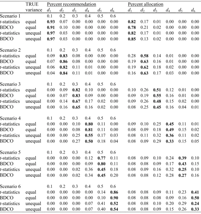
AGT activity is 5 fmol/mg protein. Data were re-sampled from Friedman et al. (1998)……….54 Table 4.2 Proportion of trials where each dose was recommended as the

target dose and proportion of subjects allocated to each dose by the t-statistics design and the new Bayesian design (BDCO). In case of unequal variances the variance of Yj is 0.12j2, j∈{1,2,3,4,5,6}, in case of equal variances the

variance is 0.2. The target value in scenario k, k = 1,…, 6 is 0.1k. Results for

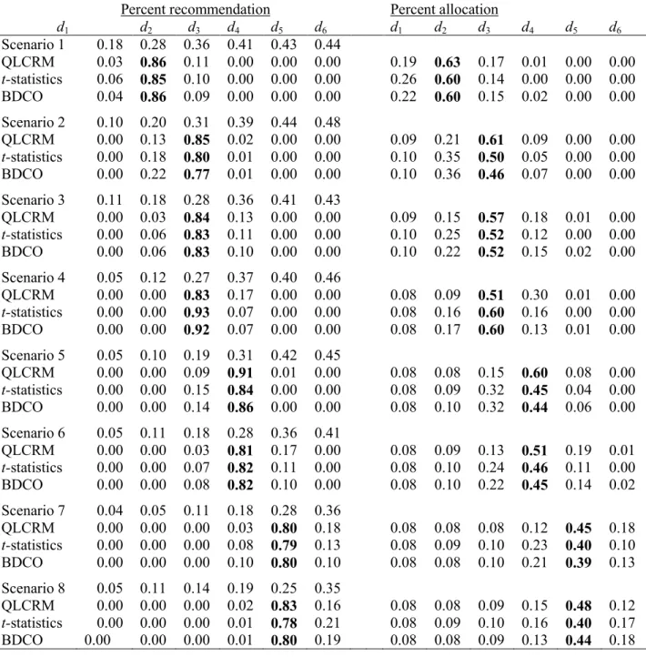
the target dose are in bold……….…55 Table 4.3 Proportion of trials where each dose was recommended as the

target dose and proportion of subjects allocated to each dose by the QLCRM, the t-statistics design and the new Bayesian design (BDCO). The target is 0.28.

xi

Table 5.2 Mean Power (SD) with constant R2………..………70 Table 5.3 Mean Power (SD) with constant β………...……….71 Table 5.4 Results for full sample (N=2983)………..73 Table 5.5 Evidence for replication in JHS using random and selective

xii

LIST OF FIGURES

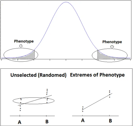
Figure 2.1 Mechanism to increase power using extreme phenotype. Select a subset of samples with extreme phenotype measures from the entire

sample. Note, removing subjects from the middle of the phenotype distribution

results in steeper regression lines than observed for the complete sample………..22

Figure 2.2 Mechanism to increase power using extreme phenotype to use

genotype extremes……….…...23 Figure 5.1 Rapid Convergence of Simulated Annealing Algorithm Irrespective

1 CHAPTER 1

LITERATURE REVIEW 1: DOSE-FINDING DESIGNS IN PHASE I CLINICAL TRIALS IN ONCOLOGY

1.1 Introduction

The primary goal for Phase I oncology trials is to find the maximally tolerable dose (MTD), the dose with certain probability of dose limiting toxicity (DLT). One important assumption for dose-finding is that the toxicity for a new intervention increases monotonically with doses in Phase I clinical trials. The toxicity associated with a dose is so called dose limiting toxicity (DLT) which is often defined as treatment related non-hematological toxicity of grade 3 or higher, or treatment related hematological toxicity of grade 4 or higher, where toxicity is measured on a scale from 0 to 5.

In Phase I oncology clinical trials, there are some issues that need be taken into considerations: ethics, delayed onset of DLT, and continuous outcome.

1) The ethical issue is the reason that we seldom use healthy volunteers and that we should neither put many patients in those doses far above MTD, nor put many patients in those doses far below MTD when the patients consent to the study wishing to find cure by taking a new treatment.

2

dose assigned to the new patients. For a traditional design, it takes a long time to finish when there is delayed onset of toxicity. Therefore traditional designs are not practical in clinical practice since doctors will not let patients waiting for treatment.

3) Another purpose of dose-finding in Phase I trials is to provide an efficacy dose of cytostatic agents for the subsequent Phase II studies though to find a MTD is a primary goal for cytotoxic agents in Phase I trials. Continuous outcomes, such as measurement of target inhibition or pharmacokinetic endpoints such as plasma drug concentrations, are usually collected in such trials. The hypothesis that toxicity increases with increased dose is not necessary true for cytostatic agents. Toxicity may happen beyond the dose to yield sufficient efficacy. New drugs may incur only moderate toxicity with no DLT being observed. Therefore, there is a need to turn the moderate toxicity into continuous scores and to find the dose targeting continuous outcome or scores.

Our goal is to develop new approaches for dose-finding design in Phase I clinical trial for both binary and continuous outcomes with better operating characteristics without or with delayed onset toxicity.

1.2 Designs or methods to solve the mentioned issues

3 1.2.1 Non-parametric designs

In non-parametric designs, no prior assumption of dose-toxicity curve is stipulated with no parameters being estimated for dose escalation. Instead, dose allocation depends on the calculated statistics such as toxicity rate estimates or t statistics according to random walk rules or up-and-down rules. The principle of these rules is that the dose for the future cohort of patient(s) is decided based on the statistics of the observed data from the previous cohort of treated patient(s). Traditional 3+3 design (Storer, 1989) which is a special form of A+B design (Lin and Shih, 2001), biased coin design (BCD) (Derman, 1957, Durham and Flournoy, 1994), group up-and-down design (Wetherill, 1963), moving average up-and-down design (Ivanova et al., 2003), group up-and-down design (Gezmu and Flournoy, 2006) are examples of non-parametric design for dose finding trials. Some of these designs, such as BCD or group up-and-down designs are Markov processes, and therefore their limiting distributions are easy to compute.

Many non-parametric designs use isotonic regression to estimate dose toxicity curve. The only assumption is that the DLT rate is nondecreasing function of the dose. These designs include isotonic design (Leung and Wang, 2001), and the Cumulative Cohort Design (Ivanova et al., 2007). The estimated toxicity rate at current dose is used to decide whether the next cohort is treated at current dose or one dose above or below. The rule for dose allocation is as follows:

i.If ˆq_j ≤ Γ − ∆, then treat the next cohort at dj+1.

ii.If ˆqj ≥ Γ + ∆, then treat the next cohort at dj-1.

iii.Otherwise, treat the next cohort at dj.

4

do not use all available data in the decision rule and therefore converge slowly to the target dose or doses near target.

1.2.2 Parametric designs for dose-finding trials

In parametric designs, the probability of DLT can be given by a multi-parameter model:

i

i d

p F_{= } _β−α _

 

where α and β is unknown shift and scale parameters (Rosenberger and Haines, 2002). The

quantile of F is _{µ α β= + F}−1_{( )Γ where Γ is a specified probability of toxicity and μ can be}

MTD. Two parameters are specified in the probability function and used in designs such as escalation with overdose control (EWOC) (Babb et al., 1998). Besides the two-parameter models, one parameter model has been also used in designs such as continual reassessment method (CRM) (O'Quigley et al., 1990).

In parametric designs, parameters are estimated using maximum likelihood or Bayesian methods. Parametric designs can be realized using maximum likelihood technique in frequentist form (O'Quigley and Shen, 1996), however, most of them belong to a class of Bayesian designs using Bayesian theorem (O'Quigley et al., 1990). A typical Bayesian decision design has four features: (a) a data model, (b) a prior distribution for parameters, (c) loss function, and (d) a set of actions (Whitehead, 2006). Decision of dose allocation is based on the posterior distribution of parameter(s) according to Bayesian theorem. To be specific, in one parameter model, the next patient is treated at the dose with the toxicity probability close to target p with parameter ϕˆbeing

calculated based on all the outcomes. The next patient will be treated at

1 arg min | ( , )ˆ ˆ|

j F dk j p

5

The CRM is a method to find MTD with certain toxicity rate for binary outcome. The one

parameter working model is

(

)

j j

P d a =b where dj is the dose, and j=1,…, K (the dose level),

and a is a parameter. In a Bayesian form of the CRM, the prior for a is specified, for example, f(a)=exp(-a). The posterior mean of parameter a is calculated using all the outcomes. Dose assignment is based on mean posterior probability that is closest to the target toxicity rate. The CRM can be used to reduce the number of patients to receive lower doses which may far below MTD as well and to achieve a more accurate estimation of MTD.

EWOC is a modified CRM in essence with safety measure to restrict a pre-specified proportion of patients to expose to a dose far above MTD. EWOC assigns doses based on the posterior probability that is overdosing. The loss function used in EWOC design is

( )

₍

(

₎₍

)

₎

x x

l x

x x

α γ γ

γ

α γ γ

 − ≤



=  _{− − >}



where γ is the parameter and γ∈[Xmin, Xmax].

Neuenschwander et al. (2008) proposed a Bayesian method which can be used to solve an overdose issue too, and defined a rule to assign dose based on maximum posterior probability within an interval. The loss function in the approach is

(

)

1

2

3

4

1 if ( ) (0,0.2] (under-dosing) 0 if ( ) (0.2,0.35] (Targeted toxicity) ,

1 if ( ) (0.35,0.6] (Excessive toxicity) 2 if

l d l d L d l d l θ θ θ π π θ π = ∈ = ∈ = = ∈

= πθ( ) (0.6,1] (Unacceptable toxicity) d       _∈ 

6

1

1 2

2

, if

( , ) , if

0, if

ε

ε ε

ε

− < −   = − ≤ − > <   ₋ 

D i T

i D i T

i T

N p p

L D p K p p

p p

1

1

2 2

, if

( , ) 0, if

, if

ε

ε ε

ε

− < − 



=_ − ≤ − <

 _{− >}



S i T

i i T

S i T

N p p

L S p p p

M p p

1

1

2 2

0, if

( , ) , if

, if

ε

ε ε

ε

− < − 



=_ − ≤ − <

 ₋

 >

i T

i E i T

E i T

p p

L E p K p p

M p p

where ( , )L D pi is the loss function for de-escalating, ( , )L S pi is for staying, and ( , )L E pi is for

escalating.

The advantage of parametric designs over non-parametric designs is that all the available information is used to determine the dose for the next patient. On the other hand, parameter designs usually are harder to understand and more difficult to use compared to non-parametric designs.

7

designs using continuous enrollment are needed to solve the problem of mandate trial suspension in traditional designs.

Several designs have been proposed to incorporate long follow-up time for toxicity in a Phase I trial. Two approaches have been used in these designs.

Cheung and Chappell (2000) assumed that time to toxicity is distributed uniformly in (0, )T given that a DLT was observed in the follow-up window of (0, T). They proposed a

modified CRM by introducing weight into the likelihood. In TITE-CRM, the dose assignment will converge to the MTD as in CRM (Cheung and Chappell, 2002). But due to rapid dose escalation, this method may end up with more patients in high toxic doses. Modifications for the TITE-CRM have been proposed by Braun et al. (2003, 2006) with the latter describing a generalization of TITE-CRM for early- and late-onset toxicities

The other approach is based on a Bayesian survival analysis methodology. This approach requires using Gibbs sampler or Markov Chain Monte Carlo (MCMC) algorithm for sampling from probability distributions through constructing a Markov chain to find the desired equilibrium distribution.

8

of administrations and the times of treatment; assumed that the general beta distribution priors for the parameters and that the hazard increases to the maximum and decrease to zero linearly, and calculated the posterior through MCMC simulation to determine the maximum tolerated schedule rather than MTD.

9 1.2.4 Dose-finding for continuous outcome

Dose limiting toxicity (yes or no) is the primary endpoint in most oncology phase I trials of cytotoxic agents. If a cytostatic agent is being investigated, toxicity is usually not a limiting factor and a continuous biomarker endpoint is often used as a primary endpoint, for example a measure of target inhibition or pharmacokinetic endpoints such as plasma drug concentrations that correlate with biological activity (Le Tourneau et al., 2009), or percentage inhibition of an enzyme (Plummer et al., 2008). Continuous endpoint also arises when multiple toxicity events in different body systems and multiple toxicity grades are combined into a single score (Bekele and Thall, 2004, Ezzalfani et al., 2012, Chen et al., 2010). A number of scores have been proposed recently, for example, total toxicity burden (TTB) (Bekele and Thall, 2004), total toxicity profile (TTP) (Ezzalfani et al., 2012), equivalent toxicity score (ETS) (Chen et al., 2010), and average toxicity score (ATS) (Bekele et al., 2010). These scores are generated through combining information from various toxicity grades, grades 1 through 5, into a single number with the goal of better reflecting toxicity burden on a patient compared to the binary outcome of dose limiting toxicity (DLT) that is usually defined as treatment related non-hematological toxicity of grade 3 or higher or treatment related non-hematological toxicity of grade 4 or higher.

10

toxicity score include t-statistics design (Ivanova and Kim, 2009), extended isotonic design (Chen et al., 2010), Quasi-CRM (Yuan et al., 2007) , Quasi-Likelihood-CRM (Ezzalfani et al., 2012) and other designs ( Lee et al., 2010).

All the methods mentioned earlier require outcome of a patient being observed quickly. In many trials, time to observe the outcome is relatively long compared to the accrual rate. In some of such trials, for example in trials where urgent treatment is needed, it is desirable to assign a dose to a patient as soon as the patient enrolls in the trial. The proposed design allows making the best possible assignment for each incoming patient using all information available.

1.3 Other related methods or rules

In this section we review several methods or rules we have seen in phase I clinical trial protocols.

1.3.1 Start-up rule

It is important to avoid escalation that is too rapid or too slow (Cheung, 2005). With that goal in mind, the group size s in the start-up should be chosen according to the target toxicity

level Γ. Ivanova et al. (Ivanova et al., 2003) suggested choosing group size according to the

following formula s= log 0.5 / log(1_

( )

used; if Γ= 0.3, the start-up with s= 2 is used; if Γ= 0.2, the start-up with s= 3 is used.

1.3.2 Isotonic regression

11

Several algorithms have been developed to compute maximum likelihood estimates under monotonic restriction. The most widely used one is pool adjacent violator algorithm (PAVA) (Barlow et al., 1972) to obtain isotonic estimates. The maximum likelihood estimates for

1

ˆ ( ,...,ˆ ˆ_K)'

µ = µ µ , can be obtained from unrestricted maximum likelihood estimates, ( ,..., )'y1 yK

for j=1,2,...,Kusing max-min formula

ˆ min max

j j

t h h h s j _{t U s L} t

h h s

n y

n

µ =

∈ ∈

=

 

 

 

=

 

 

 

∑

∑

where L_j ={1,..., }j and U_j ={ ,..., }j K

12 CHAPTER 2

LITERATURE REVIEW 2: THE USE OF SELECTIVE PHENOTYPING TO INCREASE THE POWER IN GENETICS ASSOCIATION STUDIES

2.1 Introduction

13 2.2 Genetic association studies

14 2.3 Genome-wide association studies (GWAS)

Genome-wide association studies (GWAS) that analyze the DNA variation throughout genome have become a powerful tool for investigating the role of common human genetic variation in common diseases (Bush and Moore, 2012). The goal of GWAS is to identify the variants which may be either directly causal or in linkage disequilibrium with the causal variant(s) (Hirschhorn and Daly, 2005). In GWAS, the association tests can be performed on a single locus with a single SNP, by far the most common application, or on multiple loci simultaneously with a combination of multiple SNPs (Bush et al., 2009). In these tests, logistic regression models or generalized linear regression models can be fitted for case and control studies or for quantitative trait designs, respectively, adjusted for covariates such as age, gender and principal components to control for population stratification. If family data or repeated measures are included then generalized estimating equations or linear mixed models are typically employed. Since usually over half a million SNPs are tested, a Bonferroni correction approach or a false discovery rate (FDR) procedure is used to control the rate of false positive results (Hochberg and Beniamini, 1990, van den Oord, 2008). Other procedures, such as permutation tests, are also occasionally used. It is now standard for top journals to require confirmation of new findings from a GWAS using a replication study from an additional independent sample (Chanock et al., 2007), which should repeat the design setting as close as possible and should be well-powered (Zollner and Pritchard, 2007).

2.4. Cost constraints of genotyping

15

have largely been dominated by the high cost of genotyping. The cost for genotyping a single SNP was 0.50 $, later dropped to 0.01$ (Wang et al., 2006). The average cost of genotyping one sample was initially thousands of dollars per subject, but today the cost can be as low as a couple hundred dollars or less, depending on the genetic marker panel used. Today, GWAS data are routinely available on tens of thousands of subjects from deeply phenotyped cohorts. Though the expense of phenotyping samples can also be high, since GWAS are routinely performed in large “deeply-phenotyped” community based cohorts with existing phenotype data collected from earlier epidemiological studies, the major cost constraint, to date, has been the expense of genotyping (hundreds dollar per subjects) even though the price is dropping over time.

2.5 Statistical power

16

clinical differences. The second factor is sampling error. The larger the sample variability of the test statistic the harder it is to reject the null hypothesis. Power can be improved by decreasing sampling variability of the test statistic. Increasing sample size is the primary method for reducing the sampling variation, but who is sampled can also play an important role in reducing the variation. Finally, the statistical significance threshold, i.e. the critical value for the rejection region, is an important decision in both controlling power and the type I error. Typically, greater concern is applied to controlling the type I error of the experiment. The more stringent the applied significance threshold the greater the reduction in power will be.

2.6 Extremes of phenotype for selective genotyping

17

difference under null model) and hence typically increases statistical power over similar sized random samples.

2.7 Big data era

Genome-wide genotype data have been generated on hundreds of thousands of subjects. GWAS studies are systematically being performed on existing well-phenotyped biomarkers in large cohort studies (McManus, 2009). 10’000s samples from GWAS have been deposited in dbGAP --- a database (www.ncbi.nlm.nih.gov/gap) of genotypes and phenotypes--- developed to store and distribute genotype and phenotype for association studies and methodology development from interested outside researchers (Mailman et al, 2007). Because many large cohorts have already been genotyped through GWAS, cost constraints due to genotyping will be less of a concern in the near future.

2.8 New biomarkers

18

used in in personal medicine to provide health care tailed to the individual patient (Kumar and Sarin, 2009).

2.9 Cost constraints of phenotyping

Though many biomarkers are pre-existing in large cohort studies or community based studies, not all studies are phenotyped equally. Moreover, it is often difficult to obtain sufficient funding to cover the cost of measuring new biomarkers. If there exist a priori set of genetic markers of interest that have already been genotyped, we can select a subset of subjects to phenotype that maximizes power. Such a scenario would frequently occur for replication studies, where the phenotype of interest has yet to be measured in the replication sample. Another possible scenario would be a multistage genetic association study for a new, unmeasured, biomarker where a subset of random subjects are phenotyped in stage 1 and a targeted set of subjects, based on their genotype data, are phenotyped in stage 2 for variants showing the strongest evidence of association in stage 1.

2.10 Extremes of Genotype for selective phenotyping

19

standard error of the beta estimate in the denominator. For a fixed sample size, selecting extremes of genotype should have little effect, on average, on the numerator (beyond stochastic variation) but would typically decrease the variation of the beta estimate (smaller denominator). Hence, using genotype extremes will increase our power to reject the null hypothesis in favor of the alternative, when true (Sen et al., 2009). For one marker contributing to a phenotype, it is easy to optimize the statistical power by simply choosing an equal number of the two homozygotes. However, for multiple markers contributing to a phenotype, it is a considerably more difficult problem, as there are many tradeoffs when selecting subjects. For example, a subject might have the more desirable less common homozygous genotype for one marker but have the less desirable heterozygous genotype at several of the other markers of interest. Selective phenotyping is about how to select subjects that optimizes power over a distribution of markers that are each putatively associated with a phenotype of interest.

2.11 Previous approaches in selective phenotyping

20

measuring the uncertainty about a single putative causative QTL. Selection strategy includes alternates of a selection step and a phenotyping step until the desired number of subjects is selected.

21

22

23

Figure 2.2 Mechanism to increase power using extreme phenotype to use genotype extremes

24 CHAPTER 3

THE RAPID ENROLLMENT DESIGN FOR PHASE I CLINICIAL TRIALS

3.1 Introduction

25

the beginning of the trial, may lead to assigning patients to doses with high toxicity rate when TITE-CRM is used.

In many dose-finding designs (Wetherill, 1963; Yuan and Chappell, 2004; Ivanova et al., 2007; Ivanova and Kim, 2009; Ji et al., 2010) the next assignment is determined based on the data at the current dose. We propose assigning patients at lower doses while toxicity profile at higher doses is uncertain. When assignments are being made to lower doses as well as the higher dose, it is no longer clear what dose is the current dose and therefore none of the above cited rules can be used for assignment. In this paper we describe an intuitive dose-finding method where the dose-assignment strategy is not tied to a current dose and the next assignment is made to the dose that is most likely to be the MTD. We refer to the new method as the Rapid

Enrollment Design (RED). We describe the dose-assignment design in Section 3.2. In Section 3.3 we propose how to mitigate the uncertainty from patients still in follow-up when a new assignment is made. We give an example in Section 3.4. We compare designs in Section 3.5 and discuss the findings in Section 3.6.

3.2 Dose-finding method

Let D={ ,..., }d₁ dK denote the set of ordered dose levels selected for a trial. Let T be the

length of follow-up for toxicity. A subject’s response at dk has Bernoulli distribution with

parameter qk, where (q1,…,qK) is the vector of true toxicity rates at the K doses. We assume that

q1,…,qK are non-decreasing, q1≤ ≤... qK. Observations from different subjects are independent.

Only one observation per subject is taken. The goal is to find dose dm∈D such that qm = Γ. If

there is no such dose, the goal is to find the dose d _m with mean response closest to Γ. We refer

26

First we consider the case where T is short compared to accrual rate and therefore toxicity responses from all patients are known when a new patient is enrolled. In the proposed design, each new patient is assigned to the dose with the highest probability of being the target dose

given data available so far. Let n=( ,..., )n1 nK be the number of subjects assigned to each dose

and m=( ,...,m1 mK) be the number of DLTs observed at each dose. Then the DLT rates at each

dose can be estimated by simple proportions qˆj =m nj / j, j = 1, …, K. Since qˆ1,...,qˆK might not

be monotone we will compute isotonic estimates * * 1

ˆ ˆ

( ,..., )q qK of DLT rates using the pool adjacent

violator algorithm (PAVA) (Barlow et al., 1972). PAVA is described as follows. First we set

* ˆ_j ˆ_j

q =q , j=1, …, K. If qˆ1≤ ≤... qˆK, then qˆ1*≤ ≤... qˆ*K and nothing else is needed. Otherwise, find

the smallest k such that m nk / k >mk+1/nk+1 and replace these two estimates with

* *

1 1 1

ˆk ˆk ( k k) / ( k k)

q =q + = m − +m n − +n . We also denote the estimate based on pooling data from

doses d k and dk+1 by qˆk k, 1+ with “dose” dk k, 1+ and weight nk k, 1+ =n nk + k+1. Look again for a

dose for where the working isotonic estimate is greater than the working estimate at the next higher “dose”, and repeat the averaging and concatenation process until isotonicity is actually

obtained, that is, until * * 1

ˆ ˆ_K

q ≤≤q . We note that the isotonic estimates are equivalent to the

maximum likelihood estimates assuming q1≤≤qK. In the dose-assignment design described

in the next paragraph when estimates _{( ,...,ˆ}* _ˆ* ₎ k k m

q q + , qˆ*k = =... qˆk m*+ , are computed based on pooled

data _ˆ* _{... ˆ}*

k k j

q = =q + = (mk + +... mk j+ ) / (nk+ +... nk j+ ), we use the highest dose on the estimated

plateau, dk+j , to represent the pooled doses if _ˆ* k

q ≤ Γ and the lowest dose on the estimated

plateau, dk, if _ˆ* k

27

average number of DLTs (mk + +... mk j+ ) / (j+1) and the average sample size

(nk+ +... nk j+ ) / (j+1) of the pooled doses to that dose.

To compute the probability of each dose to be the MTD we use Bayesian computations

and assume Beta(α,β) prior on qj, j= 1, 2,..., K, the posterior distribution of qj conditional on

outcome data is

| , ~ ( , )

j j j j

q m n Beta α+m β +n m− , j= 1, 2, ... , K.

The prior Beta(α,β) reflects the belief that there exists data from α β+ patients, α patients with

DLTs and β patients without a DLT. We use α =0.3 and β =0.01. This prior slows the initial

escalation because it reflects the prior DLT rate of α α β/ ( + ) 0.3 / 0.31 0.97= = , however it gets

overruled by data very soon since the effective sample size in the prior is only α β+ =0.31 of a

patient.

Let { ,..., }d1 dk be the set of doses with at least one patient assigned. The design is based

on the following rules

1)Initial escalation: do not escalate a dose unless at least s patients are assigned to current highest dose, k. The number s depends on the target rate Γ, s= 3 is often used if Γ = 0.25.

2)If _ˆ* k

q < Γ, the next patient is assigned to dk+₁ (or dK if k= K).

3)If _ˆ* k

q ≥ Γ, if there is a dose dj such that _ˆ* j

q = Γ, the next patient is assigned to dj.

Otherwise, let j, j k≤ −1, be such that _ˆ* j

q < Γ and *

1 ˆ_j

q + > Γ. Let

{

}

Pr

j qj

π = Γ − <ε < Γ −ε and π_j+1=Pr

{

}

28

4)Do not assign patients to a dose where Pr

{

}

{

}

Pr q > Γ >0.95, the trial is stopped because the lowest dose is too toxic.

5)At the end of the trial the dose that would have been recommended for the next patient is selected as the estimated MTD. No dose is selected if the lowest dose is deemed too toxic by the stopping rule.

In the rules above, ε, ε ≤min( ,1Γ − Γ), is a design parameter. We recommend ε =0.05.

Robustness of this choice is discussed in Section 3.5.

Decision rules for two candidate doses, one with estimated DLT rate lower than Γ and

one with rate higher than Γ, are shown in Table 3.1 (for Γ =0.2), Table 3.2 (for Γ =0.25) and Table 3.3 (for Γ =0.3). The first column of each of these tables contains data yielding DLT

proportion less than Γ, and the second column DLT proportion higher than Γ. The decision rule

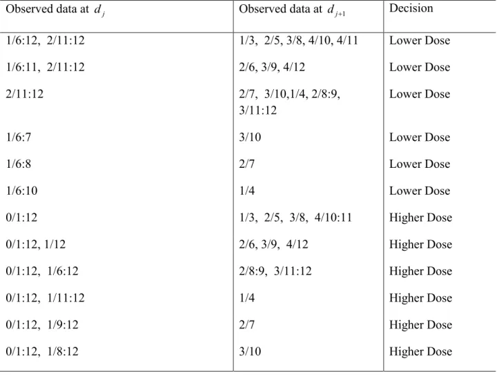
for each pair of the first and second column data is in column 3. For example, if Γ =0.2, 3 patients were enrolled at dose 1 with no DLTs, and 6 patients were enrolled at dose 2 with 2 DLTs. The decision rule for these data is to assign the higher dose (line 9, Table 3.1). This is

because the data at the two doses are (0/3, 2/6) yielding π =₁ 0.090 and π =₂ 0.181.

To implement the RED we developed web-based software available at http://www.unc.edu/wang484/red/red.php. The input is the number of DLTs at each dose,

1

( ,..., )m mk

=

m , and the number of subjects at each dose n=( ,..., )n1 nK . The program identifies

two candidate doses j and j + 1 based on isotonic estimates, and computes πj, πj+1. It also

computes the probabilities that the DLT rates at the two doses are higher than Γ needed for the

29

3.3 Mitigating uncertainty from patients still in follow-up

In many Phase I oncology trials follow-up time is long compared to accrual rate. Often 3 patients are assigned to a previously untried dose. These 3 patients need to complete follow-up at the dose before more patients can be assigned to that or higher dose level. This however, does not fully resolve uncertainty about safety of future assignments. For example, if one out of the three patients had a DLT at that dose, can we assign, say, 6 more patients to that dose at once or is it too risky? We propose a simple way to mitigate this risk. A patient with a DLT who has been in the follow-up for time u and therefore has completed a fraction u/T of the total follow-up with 1−u T/ of the follow-up still remaining is counted as a patient with 1−u T/ of a DLT. The

total DLT count at a dose is the number of actual DLTs, m, plus the sum of 1−u Ti / , where the

sum is over all the patients assigned at that dose that are still in follow-up. The denominator is the total number of patients at that dose irrespective of their follow-up time. These data are used to determine the next assignment according to the rules in Section 3.2.

For example, 3 patients have completed follow up at dose 1 with one DLT and several

patients are available to enroll. If Γ = 0.20, with 1 DTL out of 3, Pr

{

}

since this probability is less than 0.95 at least one more patient can be enrolled. If one patient is enrolled, to mitigate potential DLT outcome from this patient, the data are augmented with 1

DLT at d1 yielding 2/4 DLT at d1 and Pr

{

}

we can enroll one more patient. After augmenting 1/3 with 2/2, for two newly enrolled patients

with u= 0 follow-up each, the DTL data at d1 are 3/5 yielding Pr

{

}

cannot assign more patients to d1 at this point. After the two newly enrolled patients have been

30

0.5/1 = 2/5 yielding Pr

{

}

to d1 until the estimated DLT rate at d1 becomes lower than Γ = 0.20, at which point patients are

assigned to d2.

In another example, there are 3 patients enrolled at d1 with no DLTs, and 3 patients

enrolled at d2 with 1 DLT observed in these 3 patients. The data at the two doses are (0/3, 1/3),

corresponding to π =1 0.09 and π =2 0.15, therefore the next patient, patient seven, is assigned to

d2. If patient eight is available at the time when patient seven is assigned, the augmented data are

(0/3, 2/4), corresponding to π =₁ 0.09 and π =₂ 0.08, therefore patient eight should be assigned

to dose 1. If, instead, patient eight arrives when patient seven has completed half of his follow-up

without a DLT, the augmented data are (0/3, 1.5/4) yielding π =₁ 0.09 and π =₂ 0.14, therefore

patient 8 is assigned to d2.

3.4 Example

Dose-finding trials in acute leukemia typically require long follow-up for toxicity. This is because it is difficult to distinguish undue hematologic drug toxicity from the bone marrow effects of the disease itself. Often this requires follow-up for toxicity from an individual cycle of therapy that lasts 4-6 weeks rather than what is typical in solid tumors (3-4 weeks). In addition it is desirable to offer continuous enrollment in acute leukemia trials, since the pace of these

leukemias is so rapid that the patient may succumb to the disease while waiting. The proposed strategy was implemented in a dose-finding study of a new derivative of thalidomide for older adults with acute myeloid leukemia. Since the trial is ongoing, we used data from a recently completed Phase I trial (Foster et al., 2012) to illustrate the method. The trial investigated

31

leukemia patients. The DLT was defined as grade 3 or greater treatment-related toxicity lasting greater than 2 weeks or delay in hematologic recovery beyond 35 days from initiation of induction and not related to persistent or recurrent leukemia. Therefore the maximum

observation period for toxicity was 5 weeks from the start of therapy, and the goal of the trial was to find a dose with the DLT rate of 0.26. The trial used the time-to-event CCD method from Ivanova et al. (2007) with an ad-hoc modification that allowed rapid enrollment with immediate assignment. We illustrate how the proposed dose-assignment algorithm would have worked if used in the gemtuzumab trial. We use patient enrollment times, their DLT outcomes and the time when a DLT has occurred. There were three patients who progressed or died between days 32 and 35 without a DLT, and therefore these patients were permanently censored for DLT before T

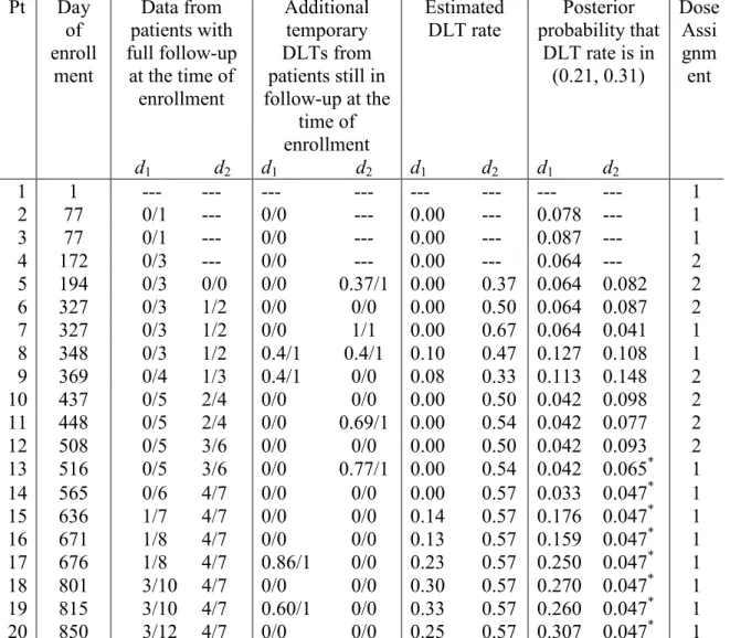
= 35. In this illustration these patients are counted as patients with full follow-up of 35 days and no DLT. Dose assignments for the first 18 patients are presented in Table 3.4. When patient 19 was enrolled, all 13 patients assigned to dose 1 have completed their follow-up and 5 DLTs were observed. The posterior probability that the DLT rate at d1 exceeds 0.26 is 0.85, and therefore

according to our method the next assignment should be to d1. In the actual acute myeloid

leukemia trial, after seeing these data, the investigators decided to be conservative and to enroll patients 19 and 20 at the lower dose, dose -1.

3.5 Comparisons with other dose-finding methods

32

The mTPI is based on computing Bayesian posterior probabilities of the DLT rate being in certain intervals. Let dj be the current dose, that is, the dose the last patient was assigned to.

Calculate three probabilities E=Pr 0

{

}

{

}

Pr j / ( )

S = Γ − <ε q < Γ +ε ε +ε and D=Pr

{

}

is assigned to dj+1 if E is the largest, to dj if S is the largest, and to dj-1 if D is the largest. If

{

}

Pr qj > Γ >0.95, patients are assigned to lower doses. If Pr

{

}

The estimated MTD is the dose with the estimated DLT rate closest to Γ.

The t-statistics method is a dose-finding design in which the t-statistic, T, to test the hypothesis that the mean at the current dose is equal to the target is computed at each step. The next patient is assigned to the current dose if −∆ < < ∆T , otherwise the dose is reduced or increased depending on the sign of T. Here Δ is a design parameter and Δ = 1 is recommended.

In the t-statistic design to estimate the target dose after the trial for the new design, we first obtained the isotonic estimates of DLT rates. The dose with the estimated DLT rate closest to Γ

is the estimated MTD. If there were two or more such doses, the highest dose with the estimated

DLT rate below Γ is chosen. If all the estimated rates at these doses were higher than Γ, the

lowest of these doses is chosen.

We used all 10 scenarios from Ji et al. (2010) to compare designs. Results for mTPI for scenarios 1, 5, 7-10 were reproduced from Ji et al. (2010) and results for scenarios 2-4 and 6 were simulated using the program provided by Yaun Ji. Simulations were performed in R and comparison is made based on 4000 simulation runs for each scenario. The target DLT rate was

0.25

Γ = _{. In all designs patients are assigned in cohorts of 3 and response is observed}

33

set α =0.3, β =0.01 and ε =0.05. Larger value of α is chosen to slow down escalation when

there is not much information available at the dose. In mTPI design the prior parameters are

1

α = , β =1 as in Ji et al. (2010). Since Ji et al. (2010), used α and β different from ours we

calibrated our safety rule so that the two designs make the same safety decision for the same data. The re-calibrated safety rule for our design is that patients are not assigned to a dose if

{

}

Pr qj > Γ >0.96.

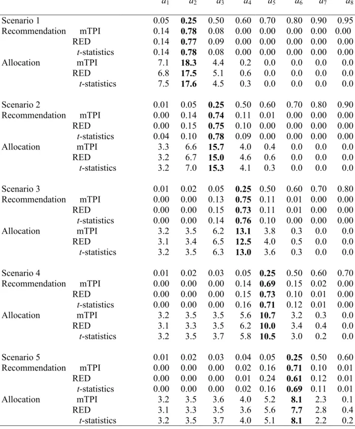
Overall all three designs perform very similarly (Table 3.5). In scenario 7 the t-statistics design recommends the target dose (dose with the DLT rate of 0.05) in 0.46 of the trials compared to 0.82 and 0.83 for the other two designs. This is because a safety rule was implemented in RED and mTPI design but not in the t-statistic design. A frequentist safety rule for the t-statistic design can be constructed similarly to the Bayesian safety rule described in Section 3.3.

We investigated the robustness of the new design with respect to parameter ε. In the main simulation study (Table 3.5) we used ε = 0.05. We performed simulations with values of

ε in the range (0.01, 0.1) and obtained very similar results (results are available from the authors).

3.5.2 Comparison with TITE-CRM when the follow-up for DLT is long

Cheung and Chappell (2000) proposed a time-to-event modification of the continual reassessment method (CRM), called TITE-CRM, for dose-finding trials where follow-up for

DLT is long. Let xi be the dose level received by subject i, xi ∈D, and yi = 1 if the ith subject had a DLT and 0 otherwise. In the original CRM (O’Quigley et al., 1990), the calculation of posterior

34

{

}

1

( ) n ( , ) 1y_i ( , ) yi,

n i i

i

L θ F x θ F x θ −

=

=

∏

where F x( , )i θ =bxθ_i and ( ,..., )b1 bK is a set of positive constants. In clinical trials that require

long follow-up times, the toxicity rate at dose xi is defined as the probability of observing

toxicity at xi during a time period of length T after initiation of therapy. Data for the ith subject,

i= 1,…, n, when (n+1)th subject is assigned to a treatment, consists of dose xi, toxicity indicator

i

y and the time ui that has elapsed from the time of the ith subject’s treatment assignment to the

time of the (n+1)th subject’s treatment assignment.

For TITE-CRM, Cheung and Chappell (2000) suggested the weighted likelihood

{

} {

}

1

( ) n ( , ) yi 1 ( , ) yi,

n i i i i

i

L θ w F x θ w F x θ −

=

=

∏



where wi is the weight assigned to the ith observation prior to the entry of the (n+1)th subject.

For example, setting wi =min( / ,1)u Ti reflects an assumption that the density of time to toxicity

is flat in (0,T).

35

Table 6 displays comparison of the two designs in a trial with 35-day follow up for DLT. Patients are assigned one at a time and enrolled at the rate of one patient per week. For patients with DLT, time to DLT was generated as uniform random variable on (0,35). We excluded scenario 8 since there is no MTD in this scenario. Due to aggressive escalation the TITE-CRM recommends the doses above the true MTD much more frequently than the RED. At the same time the recommendation of the correct dose is similar between the two designs. The RED recommends the correct MTD more often in scenarios where the MTD is among lower doses and the TITE-CRM recommends the correct MTD more often when the MTD is among higher doses. This is because the TITE-CRM escalates rapidly and the RED is conservative. Rapid escalation of the TITE-CRM to higher doses leads to observing 3 more DLTs on average in each trial compared to the RED.

The average length of a trial is 51 weeks. For comparison a trial that enrolls patients in cohorts of 3 at a time where each cohort is followed for 5 weeks before the next cohort is enrolled will have the length of approximately 70 weeks. The results of the latter are the same as those presented in Table 5. Comparison of Table 5 and 6 shows that the RED can provide good estimation of the MTD in trials with long follow-up for toxicity without exposing patients to doses with possibly high DLT rates.

3.6 Discussion

36

37

Table 3.1 Dose allocation decision based on the posterior probability at two candidate doses dj and dj+1. Target probability is Γ = 0.20. The observed toxicity rate at dj is less than Γ and the

observed toxicity rate at dj+1is higher than Γ. Data at each dose is the number of DLTs over the

number of patients assigned to the dose.

Observed data at d_j Observed data at d_j+₁ Decision

1/6:12, 2/11:12 1/3, 2/5, 3/8, 4/10, 4/11 Lower Dose

1/6:11, 2/11:12 2/6, 3/9, 4/12 Lower Dose

2/11:12 2/7, 3/10,1/4, 2/8:9,

3/11:12 Lower Dose

1/6:7 3/10 Lower Dose

1/6:8 2/7 Lower Dose

1/6:10 1/4 Lower Dose

0/1:12 1/3, 2/5, 3/8, 4/10:11 Higher Dose

0/1:12, 1/12 2/6, 3/9, 4/12 Higher Dose

0/1:12, 1/6:12 2/8:9, 3/11:12 Higher Dose

0/1:12, 1/11:12 1/4 Higher Dose

0/1:12, 1/9:12 2/7 Higher Dose

38

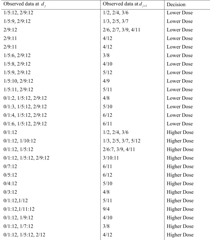
Table 3.2 Dose allocation decision based on the posterior probability at two candidate doses dj

and dj+1. Target probability is Γ = 0.25. The observed toxicity rate at djis less than Γ and the

observed toxicity rate at dj+1 is higher than Γ. Data at each dose is the number of DLTs over the

number of patients assigned to the dose.

Observed data at dj Observed data atdj+1 Decision

1/5:12, 2/9:12 1/2, 2/4, 3/6 Lower Dose

1/5:9, 2/9:12 1/3, 2/5, 3/7 Lower Dose

2/9:12 2/6, 2/7, 3/9, 4/11 Lower Dose

2/9:11 4/12 Lower Dose

2/9:11 4/12 Lower Dose

1/5:6, 2/9:12 3/8 Lower Dose

1/5:8, 2/9:12 4/10 Lower Dose

1/5:9, 2/9:12 5/12 Lower Dose

1/5:10, 2/9:12 4/9 Lower Dose

1/5:11, 2/9:12 5/11 Lower Dose

0/1:2, 1/5:12, 2/9:12 4/8 Lower Dose

0/1:3, 1/5:12, 2/9:12 5/10 Lower Dose

0/1:4, 1/5:12, 2/9:12 6/12 Lower Dose

0/1:6, 1/5:12, 2/9:12 6/11 Lower Dose

0/1:12 1/2, 2/4, 3/6 Higher Dose

0/1:12, 1/10:12 1/3, 2/5, 3/7, 5/12 Higher Dose

0/1:12, 1/5:12 2/6:7, 3/9, 4/11 Higher Dose

0/1:12, 1/5:12, 2/9:12 3/10:11 Higher Dose

0/7:12 6/11 Higher Dose

0/5:12 6/12 Higher Dose

0/4:12 5/10 Higher Dose

0/3:12 4/8 Higher Dose

0/1:12,1/12 5/11 Higher Dose

0/1:12,1/11:12 9/4 Higher Dose

0/1:12, 1/9:12 4/10 Higher Dose

0/1:12, 1/7:12 3/8 Higher Dose

39

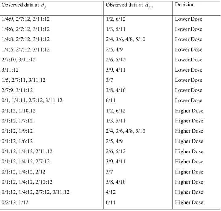
Table 3.3 Dose allocation decision based on the posterior probability at two candidate doses dj

and dj+1. Target probability is Γ = 0.30. The observed toxicity rate at djis less than Γ and the

observed toxicity rate at dj+1is higher than Γ. Data at each dose is the number of DLTs over the

number of patients assigned to the dose.

Observed data at dj Observed data at dj+1 Decision

1/4:9, 2/7:12, 3/11:12 1/2, 6/12 Lower Dose

1/4:6, 2/7:12, 3/11:12 1/3, 5/11 Lower Dose

1/4:8, 2/7:12, 3/11:12 2/4, 3/6, 4/8, 5/10 Lower Dose

1/4:5, 2/7:12, 3/11:12 2/5, 4/9 Lower Dose

2/7:10, 3/11:12 2/6, 5/12 Lower Dose

3/11:12 3/9, 4/11 Lower Dose

1/5, 2/7:11, 3/11:12 3/7 Lower Dose

2/7:9, 3/11:12 3/8, 4/10 Lower Dose

0/1, 1/4:11, 2/7:12, 3/11:12 6/11 Lower Dose

0/1:12, 1/10:12 1/2, 6/12 Higher Dose

0/1:12, 1/7:12 1/3, 5/11 Higher Dose

0/1:12, 1/9:12 2/4, 3/6, 4/8, 5/10 Higher Dose

0/1:12, 1/6:12 2/5, 4/9 Higher Dose

0/1:12, 1/4:12, 2/11:12 2/6, 5/12 Higher Dose

0/1:12, 1/4:12, 2/7:12 3/9, 4/11 Higher Dose

0/1:12, 1/4:12, 2/12 3/7 Higher Dose

0/1:12, 1/4:12, 2/10:12 3/8, 4/10 Higher Dose

0/1:12, 1/4:12, 2/7:12, 3/11:12 4/12 Higher Dose

40

Table 3.4 Dose assignments for the first 18 patients in the gemtuzumab trial. The target DLT rate is 0.26. The length of follow-up is 35 days. DLTs were observed on patients 4, 9, 11, 12, 14, 16 and 17.

Pt Day of enroll ment Data from patients with full follow-up

at the time of enrollment

Additional temporary DLTs from patients still in follow-up at the

time of enrollment

Estimated

DLT rate probability that Posterior DLT rate is in

(0.21, 0.31)

Dose Assi gnm ent

d1 d2 d1 d2 d1 d2 d1 d2

1 1 --- --- --- --- --- --- --- --- 1 2 77 0/1 --- 0/0 --- 0.00 --- 0.078 --- 1 3 77 0/1 --- 0/0 --- 0.00 --- 0.087 --- 1 4 172 0/3 --- 0/0 --- 0.00 --- 0.064 --- 2 5 194 0/3 0/0 0/0 0.37/1 0.00 0.37 0.064 0.082 2 6 327 0/3 1/2 0/0 0/0 0.00 0.50 0.064 0.087 2 7 327 0/3 1/2 0/0 1/1 0.00 0.67 0.064 0.041 1 8 348 0/3 1/2 0.4/1 0.4/1 0.10 0.47 0.127 0.108 1 9 369 0/4 1/3 0.4/1 0/0 0.08 0.33 0.113 0.148 2 10 437 0/5 2/4 0/0 0/0 0.00 0.50 0.042 0.098 2 11 448 0/5 2/4 0/0 0.69/1 0.00 0.54 0.042 0.077 2 12 508 0/5 3/6 0/0 0/0 0.00 0.50 0.042 0.093 2 13 516 0/5 3/6 0/0 0.77/1 0.00 0.54 0.042 0.065* ₁

14 565 0/6 4/7 0/0 0/0 0.00 0.57 0.033 0.047* ₁

15 636 1/7 4/7 0/0 0/0 0.14 0.57 0.176 0.047* 1 16 671 1/8 4/7 0/0 0/0 0.13 0.57 0.159 0.047* 1 17 676 1/8 4/7 0.86/1 0/0 0.23 0.57 0.250 0.047* 1 18 801 3/10 4/7 0/0 0/0 0.30 0.57 0.270 0.047* 1 19 815 3/10 4/7 0.60/1 0/0 0.33 0.57 0.260 0.047* ₁

41

Table 3.5 Comparison of the mTPI, the proposed RED method and the t-statistics design. The target DLT rate is 0.25 and the total sample size is n = 30. Proportion of times each dose is

recommended as the target dose and the average number of subjects allocated to each dose. Numbers at the target dose are in bold.

d1 d2 d3 d4 d5 d6 d7 d8

42

43

Table 3.6 Proportion of trials each dose was recommended as the MTD by the TITE-CRM and the RED. The length of follow-up for DLT is 35 days with enrollment rate of 1 patient per week.

The target DLT rate is 0.25 and the total sample size is n = 30. Numbers at the target dose are in

bold.

d1 d2 d3 d4 d5 d6 d7 d8

44

45 CHAPTER 4

DOSE-FINDING FOR CONTINUOUS OUTCOME IN PHASE I ONCOLOGY TRIALS

4.1 Introduction

Dose limiting toxicity (yes or no) is the primary endpoint in most oncology Phase I trials of cytotoxic agents. If a cytostatic agent is being investigated, toxicity is usually not a limiting factor. For example, out of 82 recent Phase I trials with cytostatic drugs reviewed by (Penel et al., 2011) dose limiting toxicity (DLT) was reached in 43 (52%) of the trials. Therefore, a continuous biomarker endpoint might be a better primary endpoint in a Phase I trial. Examples include a measure of target inhibition or pharmacokinetic endpoints such as plasma drug concentrations that correlate with biological activity (Le Tourneau et al., 2009), or percentage inhibition of an enzyme (Plummer et al., 2008).

46

score (ATS) (Bekele et al., 2010), and total toxicity profile (Ezzalfani et al., 2012). These scores are computed by combining information from various toxicity grades and various types of toxicity into a single number with the goal of better reflecting toxicity burden on a patient compared to the binary outcome of a DLT.

Dose-finding designs for continuous outcome have been proposed through controlling dose escalation via a dichotomized outcome (Mandrekar et al., 2007, Mandrekar et al., 2009, Hunsberger et al., 2005). Several methods work with the continuous endpoint directly (Ivanova and Kim, 2009, Eichhorn and Zacks, 1973). Dose-finding designs for toxicity score include quasi continual reassessment method (Yuan et al., 2007), extended isotonic design (Chen et al., 2010), the design in (Ezzalfani et al., 2012, Lee et al., 2010) and quasi-likelihood continual reassessment method of Ezzalfani et al. (2012). The t-statistics design (Ivanova and Kim, 2009) can also be used in trials with toxicity score as primary endpoint. All the methods mentioned earlier require outcome of a patient to be observed quickly. In many trials, time to observe the outcome is long compared to the accrual rate. In such trials when urgent treatment is needed, it is desirable to assign a dose to a patient as soon as the patient enrolls in the trial. The proposed design allows making the best possible assignment for each incoming patient using all information available.

In Section 4.2, we describe the proposed method. We give an example in Section 4.3. Simulation results are presented in Section 4.4 and discussion in Section 4.5.

4.2 Notation and methods 4.2.1 Probability model

Let D={ ,..., }d1 dK be the set of ordered dose levels selected for a trial. Let Yj be the

47

are unknown. The goal is to find a dose dm∈D with the mean response closest to the target

response η. We assume that mean responses are non-decreasing with dose, µ₁ ≤ ≤... µK. The

idea of the proposed design is to compute a Bayesian probability for each dose to be the target dose, that is, the probability for a dose to have the mean response close to the target η. The next assignment is made to the dose where this probability is the highest. We start with describing a Bayesian model for the data. We present the model for the case when outcome variances are

assumed to be the same 2 2 j

σ =σ _, j = 1,…, K. The case when the variances are not the same is

easier, as data from each dose is handled separately.

Ignoring the monotonicity, a conjugate prior density (Gelman et al., 1995) can be specified as

2 2

0 0

| ~ ( , / )

j N j k j

µ σ µ σ , j= 1, 2,...,K, and 2 2

0 0

~IG( , )

σ ν σ ,

where IG denotes inverse gamma distribution. Let nj be the number of subjects assigned to d_j, N

= n1 +…+ nK. The posterior of μ=( , ... ,µ1 µ ′K) conditional on σ2 and observed responses y is

2

| , ~ ( ; )

j N M Vj j

µ σ y , j= 1, 2,..., K, and 2_{| ~ ( , )}

n n IG

σ y ν σ , (1)

where M_j =(k_0jµ_0j +n_jy_j)/(k_0j +n_j), 2/( ₀ ) j j

j k n

V =σ + , ν νn= +0 N/ 2, and

0

2 2

0 0

1 0

1 _{( 1) ( )}

2

K

j j

n j j j j

j j j

k n

n s y

k n

σ σ µ

=     = + _ − + − _ +    

∑

maximum likelihood estimates of the mean response, and 2 2 1

( ,..., )s sK denoting the empirical

variances.

To impose monotonic restriction on the posterior means _{| ,}2 j

µ σ y we use the isotonic

48 1

( , ... ,µ µ ′K)

=

μ from _RK _{→ Ω to obtain the posterior distribution for the restricted means. Here}

K R

Ω ⊂ is defined by a set of vectors such that µ₁ ≤ ≤... µK . We first compute the posterior

distribution of unconstrained parameter vector μ, then obtain the draws from the posterior, and

transform draws to the constrained draws from the posterior density for the constrained

parameter vector, _μ*_{, using the pool adjacent violators algorithm (PAVA) (Barlow et al., 1972).}

From transformed draws, for each dose dj, j= 1,…, K, we compute the following probabilities

2 2 2 ( | , ), ( | , ), ( | , ) j j j j j j P P P

π η ε µ η ε σ

ρ µ η σ

τ µ η σ

= − < < + = >

= <

y y

y

The probability πj shows how likely it is that dose dj is the target dose. The probability ρj is

the probability that the mean response at djexceeds η. This probability is used to stop the trial if

the lowest dose is too toxic in trials where toxicity related outcome is the main endpoint.

Probabilities ρj and τj are useful to decide whether a dose should be inserted as described in

Section 4.2.2.

4.2.2 The Bayesian design for continuous outcomes (BDCO)

Subjects are assigned sequentially starting with the lowest dose. Similar to the start-up rule in toxicity dose-finding studies (Ivanova et al., 2003,Cheung, 2005), we recommend assigning at least three subjects to any untried dose before the dose can be escalated. Let k be the maximum dose with at least one subject assigned to it, and nj be the number of subjects assigned

to dose dj, j = 1,…, k. The next subject is assigned to the dose with the maximum probability

j