MACHINE LEARNING FOR DATA-DRIVEN BIOMEDICAL DECISION MAKING
Daniel J. Luckett
A dissertation submitted to the faculty of the University of North Carolina at Chapel Hill in partial fulfillment of the requirements for the degree of Doctor of Philosophy in the
Department of Biostatistics in the Gillings School of Global Public Health.
Chapel Hill 2018
ABSTRACT
Daniel J. Luckett: Machine Learning for Data-driven Biomedical Decision Making (Under the direction of Michael Kosorok)
The big data age has brought with it challenges and opportunities for biomedical decision making. New technologies allow for collecting large data sets that can be used to tailor treatment. In this dissertation, we develop machine learning methods for data-driven biomedical decision making with the goal of leveraging patient heterogeneity to make more precise treatment deci-sions.
Many problems in biomedical decision making can be expressed as classification problems. The costs of false positives and false negatives differ across application domains and this trade-off is often displayed using a receiver operating characteristic (ROC) curve. In the first chapter, we develop an ROC curve estimator using a weighted support vector machine (SVM).
Precision medicine is the paradigm of incorporating individual patient factors into treatment decisions, formalized through individualized treatment regimes (ITR’s), or maps from the co-variate space into the treatment space. The optimal ITR is defined as that which maximizes the mean of a clinical outcome. The estimation of an optimal ITR from mobile health data is com-plicated by the fact that observations occur over time at a fine granularity and there is no definite time horizon. In the second chapter, we develop an estimation method for optimal ITR’s in mo-bile health.
In the third chapter, we introduce a method for estimating a composite outcome from treatment decisions in observational data under the assumption that clinicians act approximately optimally.
ACKNOWLEDGEMENTS
TABLE OF CONTENTS
LIST OF TABLES . . . ix
LIST OF FIGURES . . . xi
CHAPTER 1: INTRODUCTION . . . 1
CHAPTER 2: RECEIVER OPERATING CHARACTERISTIC CURVES AND CONFIDENCE BANDS FOR SUPPORT VECTOR MACHINES. . . 6
2.1 Introduction . . . 6
2.2 Weighted Support Vector Machines . . . 8
2.2.1 ROC Curve Estimation . . . 8
2.2.2 Confidence Bands . . . 10
2.3 Theoretical Results . . . 12
2.3.1 Excess Risk and Consistency . . . 13
2.3.2 Continuity . . . 15
2.4 Simulation Experiments . . . 16
2.5 Applications to Data . . . 19
2.5.1 Breast Cancer Genomics . . . 19
2.5.2 Diagnosis of Infant Hepatitis C . . . 21
2.6 Conclusion . . . 22
CHAPTER 3: ESTIMATING DYNAMIC TREATMENT REGIMES IN MOBILE HEALTH USING V-LEARNING . . . 24
3.1 Introduction . . . 24
3.2 Offline Estimation From Observational Data . . . 26
3.4 Theoretical Results . . . 33
3.5 Simulation Experiments . . . 36
3.5.1 Greedy Gradient Q-learning . . . 36
3.5.2 Offline Simulations . . . 37
3.5.3 Online Simulations . . . 41
3.6 Case Study: Type 1 Diabetes . . . 44
3.7 Conclusion . . . 47
CHAPTER 4: ESTIMATION AND OPTIMIZATION OF COMPOSITE OUTCOMES . . . 49
4.1 Introduction . . . 49
4.2 Pseudo-likelihood Estimation of Utility Functions . . . 51
4.2.1 Fixed Utility . . . 53
4.2.2 Patient-specific Utility . . . 54
4.3 Theoretical Results . . . 56
4.4 Simulation Experiments . . . 59
4.4.1 Fixed Utility Simulations . . . 59
4.4.2 Patient-specific Utility Simulations . . . 63
4.5 Case Study: The STEP-BD Standard Care Pathway . . . 64
4.6 Conclusion . . . 69
CHAPTER 5: OUTCOME WEIGHTED LEARNING AND MAXIMUM LIKELIHOOD ESTIMATION . . . 70
5.1 Introduction . . . 70
5.2 Setup and Notation . . . 72
5.3 Outcome Weighted Learning as Maximum Likelihood . . . 73
5.4 Information Criteria for Treatment Regimes . . . 76
5.5 Simulation Experiments . . . 77
5.6 Application to Data . . . 80
CHAPTER 6: DISCUSSION AND FUTURE RESEARCH . . . 85
6.1 Discussion . . . 85
6.2 Future Research . . . 86
6.2.1 Variable Selection for SVM ROC . . . 86
6.2.2 Robust V-learning and Average Value Learning . . . 87
6.2.3 Composite Outcomes in Multiple Stages . . . 88
6.2.4 Generalized Hinge Loss and Bayesian Treatment Regimes . . . 91
APPENDIX A: TECHNICAL DETAILS FOR CHAPTER 2 . . . 93
APPENDIX B: TECHNICAL DETAILS FOR CHAPTER 3 . . . 105
APPENDIX C: TECHNICAL DETAILS FOR CHAPTER 4 . . . 114
APPENDIX D: TECHNICAL DETAILS FOR CHAPTER 5 . . . 127
LIST OF TABLES
2.1 Average AUC across simulations when true model is nonlinear. . . 17
2.2 Average coverage probabilities and area between confidence bands in simulation. . . . 18
2.3 AUC, sensitivity, and specificity of several methods applied to breast cancer data. . . 20
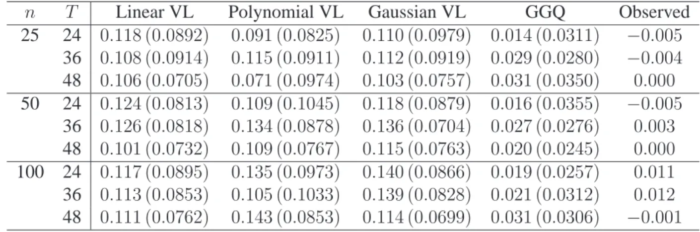
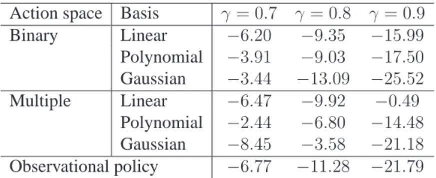
3.1 Monte Carlo value estimates for offline simulations withγ = 0.9. . . 39
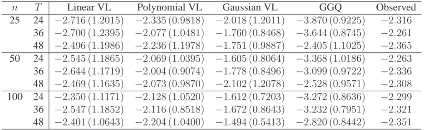
3.2 Monte Carlo value estimates for simulated T1D cohorts withγ = 0.9. . . 42
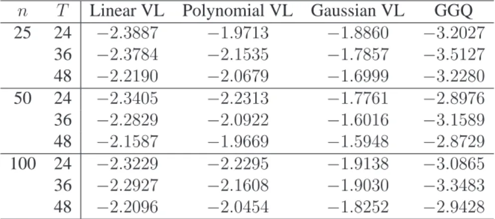
3.3 Value estimates for online simulations withγ = 0.9. . . 43
3.4 Value estimates for online estimation with simulated T1D cohorts withγ = 0.9. . . 43
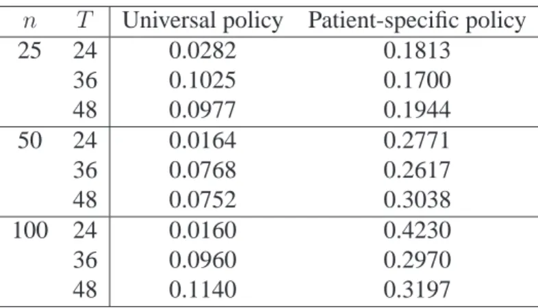
3.5 Value estimates for online simulations with universal and patient-specific poli-cies withγ = 0.9. . . 44
3.6 Parametric value estimates for V-learning applied to type 1 diabetes data. . . 46
3.7 Probabilities for each action as recommended by estimated policy for one example patient. . . 46
4.1 Estimation results for simulation where utility and probability of optimal treat-ment are fixed. . . 60
4.2 Value results for simulation where utility and probability of optimal treatment are fixed. . . 61
4.3 Estimation results for simulation where utility is fixed and probability of op-timal treatment is patient-specific. . . 62
4.4 Value results for simulation where utility is fixed and probability of optimal treatment is patient-specific. . . 62
4.5 Estimation results for simulation where utility and probability of optimal treat-ment are patient-specific. . . 63
4.6 Value results for simulation where utility and probability of optimal treatment are patient-specific. . . 64
4.8 Results of analysis of STEP-BD data with SUM-D score and SUM-M score
as outcomes. . . 67 4.9 Results of analysis of STEP-BD data with SUM-D score and side effect score
as outcomes. . . 68
5.1 Estimated MSE ofβnb across simulations when error distribution is normal. . . 78 5.2 Estimated values with Monte Carlo standard errors when error distribution
is normal. . . 79 5.3 Values of treatment policies estimated using STEP-BD data. . . 82 5.4 Coefficient estimates for assigning antidepressant or placebo from STEP-BD
data. . . 83
A.1 Average optimal sensitivity and specificity when true model is nonlinear. . . 102 A.2 Average sensitivity and specificity of unweighted SVM when true model is
nonlinear. . . 102 A.3 Average AUC when true model is linear. . . 103 A.4 Average optimal sensitivity and specificity when true model is linear. . . 103 A.5 Average sensitivity and specificity of unweighted SVM when true model is
linear. . . 104
D.1 Estimated MSE ofβnb when error distribution is Laplace. . . 131 D.2 Estimated values with Monte Carlo standard errors when error distribution
LIST OF FIGURES
2.1 Example ROC curves and confidence bands when true model is linear (left)
and nonlinear (right) in one simulated replication. . . 19 2.2 ROC curves for predicting response to breast cancer treatment using several
methods. . . 20 2.3 ROC curve and confidence bands for the linear SVM applied to diagnosing
HCV. . . 22
4.1 Box plots of log SUM-D score (severity of depression symptoms) by substance
abuse and treatment. . . 66 4.2 Box plots of log SUM-M score (severity of mania symptoms) by substance
abuse and treatment. . . 66
CHAPTER 1: INTRODUCTION
Technological advancements have lead to an increased capacity for collecting and storing large, complex data sets. These data can be used to improve the way we diagnose and treat dis-ease, thus having potential to improve patient outcomes in a variety of therapeutic areas. How-ever, taking full advantage of this potential requires the development of novel statistical methods. In this dissertation, we look at a number of problems relating to data-driven biomedical decision making and develop machine learning techniques to incorporate large and complex data sets into the way we make decisions.
2007; Kosorok and Moodie, 2015; Chakraborty and Moodie, 2013). However, additional statisti-cal tasks in precision medicine include accounting for patient covariates in diagnosis and screen-ing, discovering biomarkers that can be used to tailor treatment, identifying a subgroup that will benefit from treatment, and estimating treatment regimes to balance multiple outcomes.
In Chapter 2, we develop a fully nonparametric approach to weighted classification and show that placing unequal weight on false positives and false negatives can improve classification in many settings. Machine learning methods such as the support vector machine (SVM) are widely used in classification problems (Cortes and Vapnik, 1995; Steinwart and Christmann, 2008). Dis-playing the trade-off between false positives and false negatives is often accomplished using a receiver operating characteristic (ROC) curve (Zhou et al., 2002; Pepe, 2003). Veropoulos et al. (1999) first considered estimating an ROC curve using a weighted SVM. We build on the work of Veropoulos et al. (1999) by proposing a method to construct confidence bands for the SVM ROC curve. We prove a number of theoretical results pertaining to the weighted SVM, including uniform consistency of the risk function. We demonstrate the SVM ROC curve and confidence bands in simulation experiments and through applications to hepatitis C and breast cancer data sets.
fu-ture rewards given that patients follow a specific policy and maximize the resulting estimator over a class of policies. We show that the proposed estimators are consistent and asymptotically nor-mal under mild conditions and demonstrate the performance of V-learning through a suite of sim-ulation studies and an application to a type 1 diabetes data set.
Finally, in Chapter 5, we discuss a connection between machine learning methods and max-imum likelihood estimation and use this connection to derive new methods for estimating the optimal treatment regime. Direct search methods for the optimal treatment regime (Zhang et al., 2012b; Zhao et al., 2012; Zhou et al., 2017), represent an attractive alternative to regression-based estimators as they offer robustness to model misspecification. Direct search methods in-volve constructing an inverse probability weighted estimator (IPWE) for the mean outcome under a specific treatment regime and maximizing this estimator over a prespecified class of regimes. We show that the IPWE objective function is a profile log-likelihood function for a specific class of semiparametric models. Thus, a class of direct estimators for the optimal treatment regime can be expressed as maximum likelihood estimators. This establishes a link between machine learn-ing and maximum likelihood, or alternatively, a link between direct search and regression-based estimators. There are a number of practical advantages of this approach. First, the theoretical properties of this class of estimators can be studied by studying the class of semiparametric mod-els. Second, this approach permits a framework for discussing the efficiency of treatment regime estimators in terms of the data-generating model. Finally, this approach allows for exploratory data analysis techniques, information criteria for model selection, and a modeling setup that may be more familiar to applied researchers than an IPWE. We develop an algorithm for maximizing the proposed likelihood and demonstrate the algorithm using simulations and an application to a bipolar disorder clinical trial.
CHAPTER 2: RECEIVER OPERATING CHARACTERISTIC CURVES AND CONFIDENCE BANDS FOR SUPPORT VECTOR MACHINES
2.1 Introduction
Many important problems in biomedical decision making can be expressed as binary classi-fication problems. For example, one may wish to identify infants infected with hepatitis C virus from a sample of infants born to infected mothers (Shebl et al., 2009), screen for prostate cancer using prostate-specific antigen (Etzioni et al., 1999), or predict which breast cancer patients will respond to treatment based on genetic characteristics (Fan et al., 2011). In many scenarios, clas-sification can be improved by placing unequal weights on false positives and false negatives. We present an approach to estimating the optimal receiver operating characteristic (ROC) curve us-ing a weighted support vector machine (SVM) and introduce a bootstrap method for constructus-ing confidence bands for the SVM ROC curve.
Mac-skassy et al. (2005), and Horv´ath et al. (2008), among others. The preceding methods all assume a scalar biomarker.
A number of authors have developed methods to adapt machine learning techniques to al-low for unequal weighting of false positives and false negatives. In Example 2.5 of Steinwart and Christmann (2008), the authors discuss classification using a weighted SVM but do not vary the weights to estimate an ROC curve to inform the optimal choice of weights. Veropoulos et al. (1999) propose using weights to control the sensitivity and specificity of the SVM and estimate an ROC curve, but provide no theoretical justification or inference methods. As such, the weighted SVM has not yet been extensively applied in practice. In this paper, we build on the work of Veropoulos et al. (1999) by developing a bootstrap method for constructing confidence bands for the SVM ROC curve and providing a theoretical justification for ROC curves estimated using a weighted SVM.
There are numerous applications to motivate this work. Diagnostic tests for infant hepati-tis C virus (HCV) exhibit poor sensitivity for predicting which infants will become chronically infected. A weighted SVM using multiple biomarkers is able to improve performance over stan-dard HCV diagnostic tests. Predicting which breast cancer patients will respond to treatment is an important problem in precision medicine. Genomic data provide a wealth of information for this purpose. However, the high dimension of genomic data makes it difficult to correctly specify a model. A weighted SVM is robust to model misspecification and provides improved performance over standard classification methods.
curves (Cai and Moskowitz, 2004) and to evaluate the operating characteristics of the proposed bootstrap confidence bands. In Section 2.5, we present illustrative case studies and we conclude in Section 2.6. Proofs and additional simulation results are provided in Appendix A.
2.2 Weighted Support Vector Machines
2.2.1 ROC Curve Estimation
Assume the available data are(Ai,Xi),i = 1, . . . , n, which compriseni.i.d. copies of
(A,X), whereA ∈ {−1,1}is a class label (e.g., in diagnostic medicine,A = 1corresponds to a diseased individual andA = −1corresponds to a non-diseased individual) andX ∈ X ⊆Rp are covariates. The goal is to estimate a classifier that correctly identifies a patient’s class label based on that patient’s covariates. Consider minimizing the expected weighted misclassification, where each misclassification event is weighted by the cost functionCa(α) = {1 + (2α−1)a}/2 =
α1(a = 1) + (1−α)1(a = −1), whereCa(α)is the cost of misclassification when the true class label isA = a. In diagnostic medicine, withA = 1corresponding to disease andA = −1 corre-sponding to non-disease,αdetermines the relative weight placed on the sensitivity and specificity of the test. Whenα= 1/2, sensitivity and specificity are given equal weight and the cost function reduces to zero-one misclassification error. The optimal classifier in a class,D, is
e
Dα= arg min
D∈D E
h
1{D(X)6=A}CA(α)i, (2.1)
whereDis a class of functions mappingX into{−1,1}.
(RKHS) associated with the Gaussian kernel (Steinwart and Christmann, 2008). Minimizing the empirical risk is difficult due to the discontinuity of the indicator function. Using the hinge loss, φ(u) = max(0,1−u), as a surrogate loss function (Bartlett et al., 2006), an estimator for the optimal decision function is
b
fα = arg min
f∈F E
nφ{Af(X)}CA(α) +λnkfk2, (2.2)
wherek · kis a norm onF andλnis a penalty parameter. The problem of estimating the optimal classifier in (2.2) can be solved using the SVM introduced by Cortes and Vapnik (1995).
We estimate the optimal classifier,Dαe , usingDαb (X) = signnfαb(X)o. For anyα ∈ (0,1), we can estimate the sensitivity and specificity of the estimated classifier using the empirical es-timators given byseb fαb = En1hA= signnDαb (X)o= 1i/En1(A = 1)andspb fαb = En1hA= signnDbα(X)o=−1i/En1(A =−1). Plottingseb fbαagainst1−spb fbαas func-tions ofαwill yield a nonparametric estimator of the optimal ROC curve. There are a number of methods which can be used to select a desired value ofα, sayα∗. For example, one could choose theα∗that leads to the point on the ROC curve closest to(0,1)in Euclidean distance, theα∗ that maximizes the sum of estimated sensitivity and specificity, or theα∗ that maximizes estimated sensitivity for a fixed minimum specificity estimate (L´opez-Rat´on et al., 2014). The choice ofα∗ will depend on the clinical application of interest. We classify an individual presenting with co-variatesXasDbα∗(X). This is an equivalent formulation to the method proposed in Section 2.1 of Veropoulos et al. (1999).
Remark 2.1. The optimal classifier over all functions mappingX into{−1,1}, also known as the Bayes classifier (Duda et al., 2012), can be expressed as
D∗α(X) = signαPr(A= 1|X)−(1−α)Pr(A=−1|X) . (2.3)
Thus,D∗
ρ = Pr(A = 1). Thus, the optimal classifier given in (2.3) has the same form as the Neyman– Pearson test ofH0 : A = −1againstH1 : A = 1. If we fixkα(or equivalently, fixα) to have fixed specificitysp0, then the Neyman–Pearson lemma ensures thatDα∗(X)maximizes sen-sitivity across all classifiers with specificity equal tosp0. Therefore, the ROC curve forDα∗(X), ROC∗(u), has the property thatROC∗(u) ≥ ROC(u)for allu ∈ (0,1), whereROC(u)is the ROC curve corresponding to any other classifier. This is analogous to the result given by McIn-tosh and Pepe (2002) (see also page 169 of Pepe, 2003).
Remark 2.2. The optimal decision function inF is
e
fα = arg min
f∈F
E(1[sign{f(X)} 6=A]CA(α))
= arg min
f∈F
[ραPr{f(X)<0|A= 1}+ (1−ρ)(1−α)Pr{f(X)>0|A=−1}] = arg min
f∈F
[ρα{1−se(f)}+ (1−ρ)(1−α){1−sp(f)}]
= arg max
f∈F {
ραse(f) + (1−ρ)(1−α)sp(f)},
wherese(f)andsp(f)are the sensitivity and specificity of the decision ruleD = sign(f). Thus, the true optimal decision function maximizes a weighted sum of sensitivity and specificity where the weights are determined by the population prevalence,ρ, and a user chosen weight,α.
2.2.2 Confidence Bands
In this section, we present a method for constructing confidence bands for the ROC curve of b
fα, which provide an indication of how well the estimated classifier will perform in future sam-ples. The following result characterizes the asymptotic distribution of the estimated sensitivity of
b
fα. A proof is provided in Appendix A.
Theorem 2.1. Letsefαbbe the true sensitivity offαb and letseb fαbbe the estimated sensitiv-ity offαb, wherefαb is estimated using a linear or polynomial kernel. Then,
√
asn → ∞, whereG(α) is a mean zero Gaussian process with covariance
Eρ−21(A= 1)h1nfα1e (X)>0o−sefα1e i h1nfα2e (X)>0o−sefα2e i
−Eρ−11(A = 1)h1nfα1e (X)>0o−sefα1e i
×Eρ−11(A= 1)h1nfα2e (X)>0o−sefα2e i,
wherefαe is defined as in Remark 2.2.
An analogous result holds for the estimated specificity.
Letf pffαb = 1 − spfαbbe the false positive fraction for the decision functionfαb. Definef pf−1(·)such thatf pf−1nf pffαbo = α, i.e.,f pf−1(u)is the weightαsuch that 1−spfbα
= u. Let0 < δ < 1/2be fixed. A quantile bootstrap algorithm for constructing an asymptotically correct(1−γ)100%confidence band for the ROC curve,se{f pf−1(u)},δ < u < 1, is as follows:
1. Set a large number of bootstrap replications, B, a gridδ = z1 < . . . < zK = 1and a grid 0 =α1 < . . . < αM = 1.
2. Form = 1, . . . , M, computeRb(αm) = n1−spb fαbm
,seb fαbm
o
, the estimated ROC curve.
3. Fork = 1, . . . , K, computeyb(zk)by linearly interpolatingRb(αm). 4. Forb= 1, . . . , B:
(a) Generate a weight vectorWb,n,i = ξi/ξ, where¯ ξi, . . . , ξnare independent standard exponential random variables andξ¯=n−1Pn
i=1ξi.
(b) Form= 1, . . . , M, set
e
sebfαb=EnWb,n1 (A= 1) 1hsignnfαb(X)o= 1i
e spb
b
fα=EnWb,n1 (A=−1) 1hsignnfαb(X)o=−1i
En{Wb,n1(A=−1)},
andRbe (αm) = n1−spebfαbm
,sebe fαbm
o .
(c) Fork= 1, . . . , K, computeeyb(zk)by linearly interpolatingRbe (αm).
5. Letyep(zk)be thep-th quantile of{ybe(zk) :b = 1, . . . , B}and letp∗be the largestp∈ [0,1] such thateyp∗
/2(zk) ≤ ybe(zk) ≤ ye1−p∗
/2(zk)for allk = 1, . . . , K for at least(1− γ)B
bootstrap samples.
6. Setyℓ(zk) = yep∗
/2(zk)andyu(zk) = ey1−p∗ /2(zk).
We can also use alternate choices for the weights, for example, a multinomial weight vectorWb,n=
(Wb,n,1, . . . , Wb,n,n)⊺with probabilities(1/n, . . . ,1/n)andntrials.
By Lemmas 12.7 and 12.8 of Kosorok (2008), taking the inverse of a bounded, monotone function is Hadamard differentiable under mild regularity conditions. Thus, by Theorem 2.1 above and Theorem 2.6 of Kosorok (2008),{yℓ(zk), yu(zk)}will coverby(zk)acrossk = 1, . . . , K with probability1−γ for large enoughnandB. In addition to the linear and polynomial SVM, this procedure will work for any classifier such that the estimated decision function is in a VC class, such as a logistic regression classifier.
2.3 Theoretical Results
For anyα ∈ (0,1), the estimated classifier is the sign offαb, the minimizer of the empirical hinge loss in a classF as defined in (2.2). For anyf, defineRα(f) = E(1[sign{f(X)} 6=A]CA(α)) to be the risk off, and theφrisk off to beRα,φ(f) =E[φ{Af(X)}CA(α)]. LetR∗α = inffRα(f) andR∗α,φ = inffRα,φ(f). Finally, definefαe = arg minf∈FRα(f)andfα∗ = arg minfRα(f), i.e.,
e
fαminimizes the risk overF andf∗
α minimizes the risk over all measurable functions mapping
X intoR. None of our results require that the true minimizer,f∗
able to consistently estimate the best classifier in the class even when the model is not correctly specified.
Whenα = 0, the optimal classifier assigns−1uniformly and whenα = 1, the optimal clas-sifier assigns 1 uniformly. Focusing onα ∈ (0,1)will enable us to avoid these trivial extremes. Nonetheless, many of our results hold for allα ∈ [0,1]. We will make this distinction explicit as needed. Throughout, we assume that all requisite expectations exist.
2.3.1 Excess Risk and Consistency
The following result gives a bound on the excess risk in terms of the excessφrisk. The proof is similar to that of Theorem 3.2 of Zhao et al. (2012) and uses Theorem 1 and Example 4 of Bartlett et al. (2006). We omit the proof here. This result will be used later to show uniform con-sistency of the risk of the estimated decision function.
Lemma 2.1. For any measurablef : X → Rand any distributionP of(X, A),Rα(f)− R∗α ≤
Rα,φ(f)− R∗α,φ.
This result implies that the difference between theφrisk of the estimated decision function and the optimalφrisk is no smaller than the difference between the risk of the estimated decision function and the optimal risk. Therefore, we can consider theφrisk when proving convergence results.
Next, we establish a number of consistency results for the risk of the estimated decision func-tion. We begin with Fisher consistency. This result implies that estimation using either the hinge loss or the zero-one loss will yield the true optimal classifier given an infinite sample, providing justification for using the proposed surrogate loss function. The proof follows from an extension to the proof of Proposition 3.1 of Zhao et al. (2012) and is in Appendix A.
Theorem 2.2. For anyα ∈ [0,1], iff∗
α,φminimizesRα,φ, thenDα∗(x) = sign
f∗
α,φ(x) for almost allx∈ X.
it is uniform inα. The proof of the following result closely follows the proof of Theorem 3.3 of Zhao et al. (2012) and is in Appendix A.
Theorem 2.3. Letα∈ [0,1]be fixed and letλnbe a sequence of positive, real numbers such that λn →0andnλn → ∞. LetHkbe a RKHS with kernel functionkand letH¯kdenote the closure ofHk. Then, for any distributionP of(X, A), we have that
Rα
b fα
−inff∈H¯kRα(f)
−→P 0as n→ ∞.
We next strengthen the consistency stated above by showing that the convergence is uniform inαwhen estimation uses a linear, quadratic, polynomial, or Gaussian kernel (see Steinwart and Christmann, 2008, for a discussion of kernel functions used with the SVM). The following lemma indicates that the estimated decision function lies in a Glivenko–Cantelli class (Kosorok, 2008) indexed byα, which will help us to extend the consistency stated above to uniform consis-tency inα. The proof is in Appendix A.
Lemma 2.2. Letfαb be estimated using a linear, quadratic, polynomial, or Gaussian kernel func-tion. Then,nfαb :α∈[0,1]ois contained in a Glivenko–Cantelli (GC) class.
Given thatfbαand−fbαare contained in a GC class, we have by Corollary 9.27 (iii) of Kosorok (2008), thatφfbα
andφ−fbα
are contained in a GC class becauseφis continuous. By Corol-lary 9.27 (ii) of Kosorok (2008), we have that1(A = 1)φfαband1(A = −1)φ−fαbare contained in a GC class and thus,Lα,φfαbis contained in a GC class by Corollary 9.27 (i) of Kosorok (2008), whereLα,φ(f) =φ(Af)CA(α). It follows that
sup
α∈[0,1]
bRα,φ
b fα
− Rα,φ
b fα
P
−→0,
whereRbα,φ(f) = Enφ{Af(X)}CA(α). This convergence will be used in the proof of Theo-rem 2.4, which is given in Appendix A.
distributionP of(X, A),
sup
α∈[0,1]
Rα
b fα
− inf
f∈H¯k
Rα(f)
−→P 0 (2.4)
asn → ∞, whereHkis the RKHS associated withfαb.
Note that we do not allow the sequenceλnto depend onα, which is reflected in the implementa-tion in Secimplementa-tion 2.4 below.
2.3.2 Continuity
Here, we prove a number of continuity and convergence results regarding the ROC curve and risk function forfαe andfαb. We begin with the following result which indicates that the ROC curve of the Bayes classifier,D∗
α, is continuous. We requirePr(A = 1|X)to be a continuous random variable; however,Pr(A = 1|X)does not need to be a continuous function ofX. The proof is included in Appendix A.
Lemma 2.3. Letse∗(α) = Pr{D∗
α(X) = 1|A = 1}andsp∗(α) = Pr{Dα∗(X) = −1|A = −1} be the sensitivity and specificity ofD∗
α. Then,se∗(α)andsp∗(α)are continuous inαwhenever
Pr(A= 1|X)is a continuous random variable with support(0,1).
Thus,ROC∗(u)is monotone nondecreasing and continuous except possibly at 0. It follows from Lemma 2.3 and Remark 2.2 thatRα(fα∗)is continuous inα. This is used in the proof of the fol-lowing result, which is deferred to Appendix A.
Theorem 2.5. Under the assumptions of Lemma 2.3,Rα
e
fα, is continuous inα.
Finally, we state two corollaries pertaining to the sensitivity and specificity of the estimated decision rule. These results show that the ROC curve of the estimated decision function con-verges uniformly to the ROC curve of the optimal decision function inF. The proof of Corol-lary 2.2 relies on a novel empirical process result which is included in Appendix A.
thatαρseαe +(1−α)(1−ρ)speα =αρsefαe+(1−α)(1−ρ)spfαeandsupα∈[0,1]sefαb−seαe −→P
0andsupα∈[0,1]spfαb−speα−→P 0asn→ ∞.
Note that Corollary 2.1 does not requirefeα to be unique. We can only say that the sensitivity and specificity offαb converge to the sensitivity and specificity of a function in the same equiva-lence class asfαe, i.e., a function with optimal risk.
Corollary 2.2. Defineseb fbα
andspb fbα
as in Section 2.2 andseeαandspeα as in Corollary 2.1. Then,supα∈[0,1] bsefαb−seαe −→P 0, andsupα∈[0,1] bspfαb−speα−→P 0asn → ∞.
2.4 Simulation Experiments
To investigate the performance of classification using a weighted SVM and the resulting ROC curves and confidence bands, we use the following generative model. LetXbe generated according toX ∼ Np(µZ, σ2I), whereZis equal to a vector of ones with probabilityqand a
vector of negative ones with probability1−qandI is ap×pidentity matrix. Thus,Xis a mix-ture of multivariate normal distributions with mixing probabilityq. Letπ(X) = expit (X⊺β)
for apby 1 vectorβ. GivenX, we letAbe equal to 1 with probabilityπ(X)and−1with prob-ability1−π(X). Becauseπ(X)depends onXonly through a linear function ofX, we refer to this model below as the linear generative model. We also consider a generalization of the above model whereπ(X) = expit (X⊺β+X2
1 +X22+ 4X1X2), which we refer to below as the
nonlin-ear generative model.
We implement the weighted SVM in MATLAB software using the LIBSVM library of Chang and Lin (2011). We use both linear and Gaussian kernels. The Gaussian kernel function isk(x,y) = exp(−γkx − yk2)(Steinwart and Christmann, 2008). The bandwidth parameter,γ, and the
We compare the performance of the weighted SVM to standard methods in diagnostic medicine, including logistic regression (McIntosh and Pepe, 2002) and semiparametric ROC curves (Cai and Moskowitz, 2004). Logistic regression and the SVM combine multiple biomarkers while the semiparametric ROC curve is calculated for a single biomarker (the first component ofX). These four methods are applied to simulated data from the linear and nonlinear generative models with n = 250,500,p = 2,5,10,q = 0.05,0.25,σ = 0.75, andµ= 0.25. Whenp = 2,5, we useβ = (2,1)⊺andβ = (2,1, . . . ,1)⊺, respectively. Whenp = 10, we useβ = (2,1,1,1,1,0, . . . ,0)⊺,
i.e., noise variables are introduced for the case wherep = 10. We report the mean area under the ROC curve (AUC) and the Monte Carlo standard deviation of AUC as well as optimal sensitivity and specificity across 100 replications. Optimal sensitivity and specificity are calculated as the point on the ROC curve closest to(0,1)in Euclidean distance (see L´opez-Rat´on et al., 2014, for a discussion of different methods for selecting the optimal point on the ROC curve).
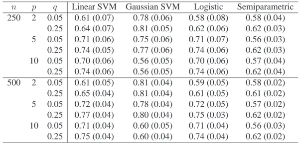
Table 2.1 below contains estimated AUC’s averaged across replications and Monte Carlo standard deviations of AUC’s for the four methods when the true generative model is nonlinear. The Gaussian SVM outperforms the other methods except in the case where there are noise
vari-n p q Linear SVM Gaussian SVM Logistic Semiparametric 250 2 0.05 0.61 (0.07) 0.78 (0.06) 0.58 (0.08) 0.58 (0.04)
0.25 0.64 (0.07) 0.81 (0.05) 0.62 (0.06) 0.62 (0.03) 5 0.05 0.71 (0.06) 0.75 (0.06) 0.71 (0.07) 0.56 (0.03) 0.25 0.74 (0.05) 0.77 (0.06) 0.74 (0.06) 0.62 (0.03) 10 0.05 0.70 (0.06) 0.56 (0.05) 0.70 (0.06) 0.57 (0.04) 0.25 0.74 (0.06) 0.56 (0.05) 0.74 (0.06) 0.62 (0.04) 500 2 0.05 0.61 (0.05) 0.81 (0.04) 0.59 (0.05) 0.58 (0.02) 0.25 0.65 (0.04) 0.81 (0.04) 0.61 (0.05) 0.61 (0.02) 5 0.05 0.72 (0.04) 0.78 (0.04) 0.72 (0.05) 0.57 (0.02) 0.25 0.77 (0.04) 0.80 (0.04) 0.75 (0.03) 0.62 (0.02) 10 0.05 0.71 (0.04) 0.60 (0.05) 0.71 (0.04) 0.56 (0.03) 0.25 0.75 (0.04) 0.60 (0.04) 0.74 (0.04) 0.62 (0.02) Table 2.1: Average AUC across simulations when true model is nonlinear.
gen-erative model is nonlinear, averaged across replications. Table A.2 in Appendix A contains esti-mated sensitivities and specificities of an unweighted SVM when the true model is nonlinear. The unweighted SVM often fails to achieve a balance between sensitivity and specificity. In particular, the linear SVM often achieves low specificity. The imbalance between sensitivity and specificity is often worse whenqis small, indicating that proper balance is difficult to achieve when there is an imbalance between true class labels in the data. These results highlight the importance of estimating the full ROC curve and selecting the weight to achieve the desired balance between sensitivity and specificity; unweighted classification may not achieve satisfactory performance in many settings. Tables A.3, A.4, and A.5 in Appendix A contain results when the true generative model is linear.
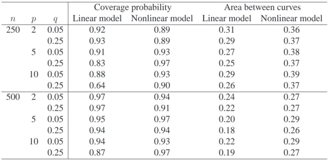
Next, we examine the performance of the bootstrap confidence band method for the linear SVM. Independent testing sets of size 100,000 were used to calculatesefαbandspfαb, giv-ing us an approximation to the true ROC curve for eachfαb. The method introduced in Section 2.2.2 was used to construct 90% confidence bands using 1000 bootstrap samples. We report the propor-tion of 100 Monte Carlo replicapropor-tions for which the true ROC curve is fully contained within the confidence band across [0.01, 0.99] along with the average area between the upper and lower con-fidence bands. Table 2.2 contains these results. We observe that, acrossn,p, andq, the proposed
Coverage probability Area between curves n p q Linear model Nonlinear model Linear model Nonlinear model
250 2 0.05 0.92 0.89 0.31 0.36
0.25 0.93 0.89 0.29 0.37
5 0.05 0.91 0.93 0.27 0.38
0.25 0.83 0.97 0.25 0.37
10 0.05 0.88 0.93 0.29 0.39
0.25 0.64 0.90 0.26 0.37
500 2 0.05 0.97 0.94 0.24 0.27
0.25 0.97 0.91 0.22 0.27
5 0.05 0.95 0.97 0.20 0.29
0.25 0.94 0.94 0.18 0.26
10 0.05 0.94 0.93 0.22 0.29
0.25 0.87 0.97 0.19 0.27
quantile bootstrap method provides approximately 90% coverage with the area between curves decreasing for larger sample sizes.
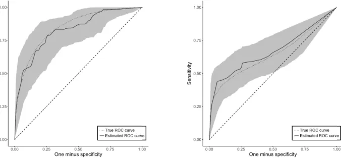
Figure 2.1 below contains bootstrap confidence bands for one simulated replication for the linear and nonlinear generative model whenn = 500,p = 2, andq = 0.25. The true ROC curve, calculated from a large testing set of size 100,000, is also plotted. These figures
demon-0.00 0.25 0.50 0.75 1.00
0.00 0.25 0.50 0.75 1.00
One minus specificity
Sensitivity
Estimated ROC curve
0.00 0.25 0.50 0.75 1.00
0.00 0.25 0.50 0.75 1.00
One minus specificity
Sensitivity
Estimated ROC curve
Figure 2.1: Example ROC curves and confidence bands when true model is linear (left) and nonlinear (right) in one simulated replication.
strate that the proposed quantile bootstrap produces confidence bands that capture the true ROC curve and are sufficiently narrow as to provide useful inference about the future performance of an estimated SVM classifier.
2.5 Applications to Data
2.5.1 Breast Cancer Genomics
variables. Figure 2.2 contains ROC curves for predicting response to treatment using the linear and Gaussian SVM, logistic regression with LASSO penalty (Tibshirani, 1996), and random forests (Breiman, 2001). Confidence bands for the linear SVM are also plotted. Each method
0.00 0.25 0.50 0.75 1.00
0.00 0.25 0.50 0.75 1.00
One minus specificity
Sensitivity
Figure 2.2: ROC curves for predicting response to breast cancer treatment using several methods.
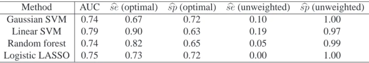
performs equally well, with each ROC curve falling within the confidence bands for the linear SVM. Table 2.3 contains AUC and optimal sensitivity and specificity for each method along with the sensitivity and specificity of the unweighted versions of each method. On these data, the
lin-Method AUC seb (optimal) spb (optimal) seb (unweighted) spb (unweighted)
Gaussian SVM 0.74 0.67 0.72 0.10 1.00
Linear SVM 0.79 0.90 0.63 0.19 0.97
Random forest 0.74 0.82 0.65 0.05 0.99
Logistic LASSO 0.75 0.73 0.72 0.00 1.00
Table 2.3: AUC, sensitivity, and specificity of several methods applied to breast cancer data.
2.5.2 Diagnosis of Infant Hepatitis C
Finally, we apply the proposed methods to data from the cohort study of mother-to-infant hepatitis C transmission of Shebl et al. (2009). In this study, 1863 mother-infant pairs in three Egyptian villages were studied to assess risk factors for vertical transmission of hepatitis C virus (HCV). Of this sample, 33 infants were positive for both HCV RNA and HCV antibodies at the end of the study. We use data from infant follow-up visits at 2-4 months and 10-12 months. At each follow-up visit, infants were tested for HCV RNA using a polymerase chain reaction (PCR) test and HCV antibodies using an enzyme-linked immunosorbent assay (ELISA) test. Mothers in the study were also tested for HCV RNA and antibodies during pregnancy. In pediatric infec-tious diseases, it is of interest to diagnose infected infants as early in life as possible so that they can benefit from early treatment with antivirals as they become approved for children— that is, we seek a highly sensitive test. We use a weighted SVM to estimated a classifier based on the mother’s test results during pregnancy and infant’s test results at 2-4 months. While a PCR test at 2-4 months detects HCV viremia, it cannot predict which children subsequently become chroni-cally infected, and a PCR test at 10-12 months remains the gold standard.
In this study, the PCR test achieved a sensitivity of 0.4167 and a specificity of 0.9911. The ELISA test achieved a sensitivity of 0.5833 and a specificity of 0.9571. Due to a variety of fac-tors, diagnosis during the early months of life is difficult. Both PCR and ELISA suffer from low sensitivity at 2-4 months for detecting which infants will become chronically infected later. It is of interest to see if diagnosis via a weighted SVM can provide even a modest improvement in per-formance, particularly an increase in sensitivity, thereby reducing the need for a repeat test after 10-12 months of age.
0.00 0.25 0.50 0.75 1.00
0.00 0.25 0.50 0.75 1.00
One minus specificity
Sensitivity
Figure 2.3: ROC curve and confidence bands for the linear SVM applied to diagnosing HCV.
0.8000, which provides increased sensitivity and a better balance between sensitivity and speci-ficity when compared to the usual diagnostic tests. Classification is difficult due to the imbalance of infections and non-infections in the data, but a weighted SVM provides increased performance compared to either diagnostic test available.
2.6 Conclusion
demon-strated its performance in simulation studies, and provided a bootstrap confidence band method for the SVM ROC curve.
The applications of the weighted SVM in diagnostic medicine are numerous. We have demon-strated, for example, that this method can be used to improve early infant diagnosis of hepatitis C. Early detection of childhood infectious diseases is an important public health problem; reliable early diagnosis identifies children who could transmit the virus and would benefit from treatment with antivirals. We have also demonstrated that the weighted SVM accommodates high dimen-sional data and can be used to predict response to neoadjuvant breast cancer treatment using ge-nomic information.
CHAPTER 3: ESTIMATING DYNAMIC TREATMENT REGIMES IN MOBILE HEALTH USING V-LEARNING
3.1 Introduction
The use of mobile devices in clinical care, called mobile health (mHealth), provides an effec-tive and scalable platform to assist patients in managing their illness (Free et al., 2013; Steinhubl et al., 2013). Advantages of mHealth interventions include real-time communication between a patient and their health-care provider as well as systems for delivering training, teaching, and social support (Kumar et al., 2013). Mobile technologies can also be used to collect rich longitu-dinal data to estimate optimal dynamic treatment regimes and to deliver treatment that is deeply tailored to each individual patient. We propose a new estimator of an optimal treatment regime that is suitable for use with with longitudinal data collected in mHealth applications.
momentary signal may be weak and may not directly measure the outcome of interest; and esti-mation of optimal treatment strategies must be done online as data accumulate.
This work is motivated in part by our involvement in a study of mHealth as a management tool for type 1 diabetes. Type 1 diabetes is an autoimmune disease wherein the pancreas pro-duces insufficient levels of insulin, a hormone needed to regulate blood glucose concentration. Patients with type 1 diabetes are continually engaged in management activities including monitor-ing glucose levels, timmonitor-ing and dosmonitor-ing insulin injections, and regulatmonitor-ing diet and physical activity. Increased glucose monitoring and attention to self-management facilitate more frequent treatment adjustments and have been shown to improve patient outcomes (Levine et al., 2001; Haller et al., 2004; Ziegler et al., 2011). Thus, patient outcomes have the potential to be improved by diabetes management tools which are deeply tailored to the continually evolving health status of each pa-tient. Mobile technologies can be used to collect data on physical activity, glucose, and insulin at a fine granularity in an outpatient setting (Maahs et al., 2012). There is great potential for us-ing these data to create comprehensive and accessible mHealth interventions for clinical use. We envision application of this work for use before the artificial pancreas (Weinzimer et al., 2008; Kowalski, 2015; Bergenstal et al., 2016) becomes widely available.
we call V-learning, involves estimating the optimal policy among a prespecified class of policies (Zhang et al., 2012b, 2013). It requires minimal assumptions about the data-generating process and permits estimating a randomized decision rule that can be implemented online as data accu-mulate.
In Section 3.2, we describe the setup and present our method for offline estimation using data from a micro-randomized trial or observational study. In Section 3.3, we extend our method for application to online estimation with accumulating data. Theoretical results, including consis-tency and asymptotic normality of the proposed estimators, are presented in Section 3.4. We com-pare the proposed method to GGQ using simulated data in Section 3.5. A case study using data from patients with type 1 diabetes is presented in Section 3.6 and we conclude with a discussion in Section 3.7. Proofs of technical results are in Appendix B.
3.2 Offline Estimation From Observational Data
We assume that the available data are S1i, A1
i,S2i, . . . ,S Ti
i , A Ti
i ,S Ti+1
i
n
i=1, which
com-prise independent, identically distributed trajectories S1, A1,S2, . . . ,ST, AT,ST+1, where:
St ∈ Rp denotes a summary of patient information collected up to and including timet;At ∈ A denotes the treatment assigned at timet; andT ∈ Z+denotes the (possibly random) patient follow-up time. In the motivating example of type 1 diabetes,Stcould contain a patient’s blood glucose, dietary intake, and physical activity in the hour leading up to timetandAtcould de-note an indicator that an insulin injection is taken at timet. We assume that the data-generating model is a time-homogeneous Markov process so thatSt+1 ⊥⊥ (At−1,St−1, . . . , A1,S1)(At,St) and the conditional densityp(st+1|at,st)is the same for allt ≥ 1. LetLt ∈ {0,1}denote an indicator that the patient is still in follow-up at timet, i.e.,Lt = 1if the patient is being followed at timetand zero otherwise. We assume thatLtis contained inStso thatP(Lt+1 = 1|At,St, . . . , A1,S1) = P(Lt+1 = 1|At,St)andLt = 0impliesLt+1 = 0with
sub-sequently transitioning to stateSt+1. In our motivating example, the utility at timetcould be a measure of how far the patient’s average blood glucose concentration deviates from the optimal range over the hour preceding and following timet. The goal is to select treatments to maximize expected cumulative utility; treatment selection is formalized using a treatment regime (Schulte et al., 2014; Kosorok and Moodie, 2015) and the utility associated with any regime is defined us-ing potential outcomes (Rubin, 1978).
LetB(A)denote the space of probability distributions overA. A treatment regime in this context is a functionπ : domSt → B(A)so that, underπ, a decision maker presented with state St = stat timetwill select actionat ∈ Awith probabilityπ(at;st). Defineat = (a1, . . . , at) ∈
At, anda∞ = (a1, a2, . . .)∈ A∞. The set of potential outcomes is
W∗ =nS1,S∗2(a1), . . . ,S∗T∗(a∞)(aT∗(a∞)−1) :
T∗(a∞) = inft ≥1 : L∗t(at−1) = 0 , a∞ ∈ A∞o,
whereS∗t(at−1)is the potential state andL∗t(at−1)is the potential follow-up status at timet
un-der treatment sequenceat−1. Thus, the potential utility at timetis
U∗t(at) =uS∗(t+1)(at), at,S∗t(at−1) .
For anyπ, define{ξt
π(·)}t≥1 to be a sequence of independent,A-valued stochastic processes
in-dexed bydomStsuch thatP {ξt
π(st) = at} = π(at;st). The potential follow-up time underπ is
T∗(π) =X
t≥1
X
at∈At
t1supat+1T∗(at, at+1) =t t Y
v=1
1ξπvS∗v(av−1) =av,
whereat+1 = (at+1, at+2, . . .). The potential utility underπat timetis
U∗t(π) =
P
at∈AtU∗t(at)
Qt
v=11 [ξπv{S∗v(av−1)}=av], if T∗(π)≥t
whereS∗1(a0) = S1. Thus, utility is set to zero after a patient is lost to follow-up. However, in
certain situations, utility may be constructed so as to take a negative value at the time point when the patient is lost to follow-up, e.g., if the patient discontinues treatment because of a negative effect associated with the intervention. Define the state-value function
V(π,st) =E (
X
k≥0
γkU∗(t+k)(π)St=st )
(Sutton and Barto, 1998), whereγ ∈ (0,1)is a fixed constant that captures the trade-off between short- and long-term outcomes. For any distributionRondomS1, define the value function with respect to reference distributionRasVR(π) = R V(π,s)dR(s); throughout, we assume that this reference distribution is fixed. The reference distribution can be thought of as a distribution of initial states and we estimate it from the data in the implementation in Sections 3.5 and 3.6. For a prespecified class of regimes,Π, the optimal regime,πoptR ∈Π, satisfiesVR(πoptR )≥ VR(π)for all π ∈Π.
To construct an estimator ofπRopt, we make a series of assumptions that connect the potential outcomes inW∗with the data-generating model.
Assumption 3.1. Strong ignorability,At ⊥⊥W∗Stfor allt.
Assumption 3.2. Consistency,St=S∗t(At−1)for alltandT =T∗(A∞).
Assumption 3.3. Positivity, there existsc0 >0so thatP(At =at|St =st) ≥ c0 for allat ∈ A,
st∈domSt, and allt.
In addition, we implicitly assume that there is no interference among the experimental units. These assumptions are common in the context of estimating dynamic treatment regimes (Robins, 2004; Schulte et al., 2014). Assumptions 3.1 and 3.3 hold by construction in a micro-randomized trial (Klasnja et al., 2015; Liao et al., 2015).
data. The following lemma characterizesVR(π)for any regime,π, in terms of the data-generating model (see also Lemma 4.1 of Murphy et al., 2001). A proof is provided in Appendix B.
Lemma 3.1. Letπdenote an arbitrary regime andγ ∈ (0,1)a discount factor. Then, under assumptions 3.1-3.3 and provided interchange of the sum and integration is justified, the state-value function ofπatstis
V(π,st) = X
k≥0
E "
γkUt+k ( k
Y
v=0
π(Av+t;Sv+t) µv+t(Av+t;Sv+t)
)
St=st #
. (3.1)
The preceding result will form the basis for an estimating equation forVR(π). Write the right hand side of (3.1) as
V(π,St) = E (
π(At;St) µt(At;St) U
t+γX k≥0
E "
γkUt+k+1 ( k
Y
v=0
π(Av+t+1;Sv+t+1)
µv+t+1(Av+t+1;Sv+t+1)
)
St+1
#! St ) = E
π(At;St) µt(At;St)
Ut+γV(π,St+1)
St ,
from which it follows that
0 =E
π(At;St) µt(At;St)
Ut+γV(π,St+1)−V(π,St)
St .
Subsequently, for any functionψ defined ondomSt, the state-value function satisfies
0 =E
π(At;St) µt(At;St)
Ut+γV(π,St+1)−V(π,St) ψ(St)
, (3.2)
which is an importance-weighted variant of the well-known Bellman optimality equation (Sutton and Barto, 1998).
LetV(π,s;θπ)denote a model forV(π,s)indexed byθπ ∈ Θ ⊆ Rq. We assume that the mapθπ 7→ V(π,s;θπ)is differentiable everywhere for each fixedsandπ. Let∇
denote the gradient ofV(π,s;θπ)and define
Λn(π, θπ) =
1 n n X i=1 Ti X t=1
π(At i;Sti) µt(At
i;Sti)
Uit+γV(π,Sti+1;θπ)−V(π,Sti;θπ)
× ∇θπV(π,St
i;θπ). (3.3)
Given a positive definite matrixΩ ∈ Rq×qand penalty functionP : Rq → R+, defineθbπ n =
arg minθπ∈Θ{Λn(π, θπ)⊺ΩΛn(π, θπ) +λnP(θπ)}, whereλnis a tuning parameter. Subsequently,
V π,s;θbπ n
is the estimated state-value function underπin states. Thus, given a reference dis-tribution,R, the estimated value of a regime,π, isVn,Rb (π) = R V π,s;bθπ
n
dR(s)and the esti-mated optimal regime isbπn = arg maxπ∈ΠVn,Rb (π). The idea of V-learning is to use estimating
equation (3.3) to estimate the value of any policy and maximize estimated value over a class of policies; we will discuss strategies for this maximization in Section 3.5.
V-learning requires a parametric class of policies. Assuming that there areK possible treat-ments,a1, . . . , aK, we can define a parametric class of policies as follows. Define
π(aj;s, β) = exp(s⊺βj)/
(
1 +
K−X1
k=1
exp(s⊺βk)
)
forj = 1, . . . , K −1, and
π(aK;s) = 1/ (
1 +
K−X1
k=1
exp(s⊺βk)
) .
This defines a class of randomized policies parametrized byβ = (β⊺
1, . . . , β
⊺
K−1)⊺, whereβkis
a vector of parameters for thek-th treatment. Under a policy in this class defined byβ, actions are selected stochastically according to the probabilitiesπ(aj;s, β),j = 1, . . . , K. In the case of a binary treatment, a policy in this class reduces toπ(1;s, β) = exp(s⊺β)/
{1 + exp(s⊺β)
}
andπ(0;s, β) = 1/{1 + exp(s⊺β)
V-learning also requires a class of models for the state value function indexed by a parameter, θπ. We use a basis function approximation. LetΦ = (φ
1, . . . , φq)⊺be a vector of prespecified basis functions and letΦ(sti) = {φ1(sti), . . . , φq(sti)}⊺. LetV(π,st
i;θπ) = Φ(sti)⊺θπ. Under this working model,
Λn(π, θπ) = "
n−1 n X i=1 Ti X t=1
π(At i;Sti) µt(At
i;Sti)
γΦ(Sti)Φ(Sti+1)⊺
−Φ(Sti)Φ(Sti)⊺
# θπ
+n−1 n X i=1 Ti X t=1 π(At
i;Sti) µt(At
i;Sti)
UitΦ(Sti)
.
Computational efficiency is gained from the linearity ofV(π,sti;θπ)inθπ; flexibility can be achieved through the choice ofΦ. We examine the performance of V-learning using a variety of basis functions in Sections 3.5 and 3.6.
3.3 Online Estimation From Accumulating Data
Suppose we have accumulating data{(S1i, A1
i,S2i, . . .)} n
i=1, whereSti andAtirepresent the state and action for patienti= 1, . . . , nat timet ≥1. At each timet, we estimate an optimal pol-icy in a class,Π, using data collected up to timet, take actions according to the estimated optimal policy, and estimate a new policy using the resulting states. Letbπt
nbe the estimated policy at time t, i.e.,πbt
nis estimated after observing stateSt+1 and before taking actionAt+1. IfΠis a class of randomized policies, we can select an action for a patient presenting withSt+1 = st+1according toπbt
n(·;st+1), i.e., we drawAt+1according to the distributionP(At+1 = a) = πbnt(a;st+1). If a class of deterministic policies is of interest, we can inject some randomness intobπt
At each timet ≥ 1, letbθπ
n,t = arg minθπ∈Θ{Λn,t(π, θπ)⊺ΩΛn,t(π, θπ) +λnP(θπ)}, whereΩ,
λn, andP are as defined in Section 3.2 and
Λn,t(π, θπ) =
1
n n X
i=1
t X
v=1
π(Av i;Svi) b
πv−1
n (Avi;Svi)
Uiv+γV(π,Svi+1;θπ)−V(π,Svi;θπ)
× ∇θπV(π,Sv
i;θπ) (3.4)
withbπ0
nsome initial randomized policy. We note that estimating equation (3.4) is similar to (3.3), except thatπbv−1
n replacesµv as the data-generating policy. Given the estimator of the value of πat timet,Vn,R,tb (π) = R V π,s;bθπ
n,t
dR(s), the estimated optimal policy at timetisbπt n =
arg maxπ∈ΠVn,R,tb (π). In practice, we may choose to update the policy in batches rather than at every time point. An alternative way to encourage exploration through the action space is to chooseπbt
n = arg maxπ∈Π
n b
Vn,R,t(π) +αtψbt(π)ofor some sequenceαt ≥ 0, whereψbt(π)is a measure of uncertainty inVn,R,tb (π). An example of this is upper confidence bound sampling, or UCB (Lai and Robbins, 1985).
It some settings, when the data-generating process may vary across patients, it may be de-sirable to allow each patient to follow an individualized policy that is estimated using only that patient’s data. Suppose thatnpatients are followed for an initialT1time points after which the
policybπ1
nis estimated. Then, suppose that patientifollowsπbn1 until timeT2, when a policybπi2is estimated using only the states and actions observed for patienti. This procedure is then carried out until timeTK for some fixedK with each patient following their own individual policy which is adapted to match the individual over time. We may also choose to adapt the randomness of the policy at each estimation. For example, we could selectǫ1 > ǫ2 > . . . > ǫK and, following esti-mationk, have patientifollow policyπbk
3.4 Theoretical Results
In this section, we establish asymptotic properties ofθbπ
n andbπnfor offline estimation. Through-out, we assume assumptions 3.1-3.3 from Section 3.2.
Letθbπ
n = arg minθπ∈Θ{Λn(π, θπ)⊺Λn(π, θπ) +λn(θπ)⊺θπ}. Thus, we use the squared
Eu-clidean norm ofθas the penalty function; we will assume thatλn = oP(n−1/2). For
simplic-ity, we letΩbe the identity matrix. Assume the working model for the state value function in-troduced in Section 3.2, i.e.,V(π,sti;θπ) = Φ(st
i)⊺θπ. For fixedπ, denote the trueθπ byθπ0,
i.e.,V(π,s) = Φ(s)⊺θπ
0. Letν =
R
Φ(s)dR(s)so thatVR(π) = ν⊺θπ
0. DefineVbn,Rb(π) = {EnΦ(S)}⊺b
θπ
n, whereEndenotes the empirical measure. LetΠ = {πβ :β ∈ B}be a parametric class of policies and letbπn=πβbn whereβnb = arg maxβ∈BVbn,Rb(πβ).
Our main results are summarized in Theorems 3.1 and 3.2 below. Because each patient tra-jectory is a stationary Markov chain, we need to use asymptotic theory based on stationary pro-cesses; consequently, some of the required technical conditions are more difficult to verify than those for i.i.d. data. Define the bracketing integral for a class of functions,F, byJ[]{δ,F, Lr(P)}= Rδ
0
p
logN[]{ǫ,F, Lr(P)}dǫ, where the bracketing number forF,N[]{ǫ,F, Lr(P)}, is the num-ber ofLr(P)ǫ-brackets needed such that each element ofF is contained in at least one bracket (see Chapter 2 of Kosorok, 2008). For any stationary sequence of possibly dependent random variables,{Xt}
t≥1, letMcbbe theσ-field generated byXb, . . . , Xc and define
ζ(k) = E
sup
m≥1
|P(B|Mm
1 )−P(B)|:B ∈ M∞m+k
.
We say that the chain{Xt}
t≥1 is absolutely regular ifζ(k) → 0ask → 0(also calledβ-mixing
in Chapter 11 of Kosorok, 2008). We make the following assumptions. Assumption 3.4. There exists a2< ρ <∞such that
1. E|Ut|3ρ <∞,EkΦ(St)k3ρ<∞, andEkStk3ρ<∞.
2. The sequence{(St, At)}
3. The bracketing integral of the class of policies,J[]{∞,Π, L3ρ(P)}<∞. Assumption 3.5. There exists somec1 >0such that
inf
π∈Πc
⊺E
π(At;St) µt(At;St)
Φ(St)Φ(St)⊺
−γ2Φ(St+1)Φ(St+1)⊺
c≥c1kck2
for allc∈Rq.
Assumption 3.6. The mapβ 7→VR(πβ)has a unique and well separated maximum overβ in the interior ofB; letβ0denote the maximizer.
Assumption 3.7. The following holds: supkβ1−β2k≤δEkπβ1(A;S)−πβ2(A;S)k →0asδ↓0. Remark 3.1. Assumption 3.4 requires certain finite moments and that the dependence between observations on the same patient vanishes as observations become further apart. In Lemma B.2 in Appendix B, we verify part 3 of assumption 3.4 and assumption 3.7 for the class of policies introduced in Section 3.2. However, note that the theory holds for any class of policies satisfy-ing the given assumptions, not just the class considered here. Assumption 3.5 is needed to show the existence of a uniqueθπ
0 uniformly overΠand assumption 3.6 requires that the true optimal
decision in each state is unique (see assumption A.8 of Ertefaie, 2014). Assumption 3.7 requires smoothness on the class of policies.
The main results of this section are stated below. Theorem 3.1 states that there exists a unique solution to0 = EΛn(π, θπ)uniformly overΠand that the estimatorθnb converges weakly to a mean zero Gaussian process inℓ∞(Π).
Theorem 3.1. Under the given assumptions, the following hold.
1. For allπ ∈Π, there exists aθ0π ∈Rqsuch thatEΛn(π, θπ)has a zero atθπ =θπ0. Moreover, supπ∈Πkθπ
0k<∞andsupkβ1−β2k≤δ θπβ1
0 −θ
πβ2 0
2. LetG(π)be a tight, mean zero Gaussian process with covarianceE{G(π1)G(π2)} = w1(π1)−1w0(π1, π2)w1(π2)−⊺, indexed byΠ, where
w0(π1, π2) = E
π1(At;St)π2(At;St) µt(At;St)2
Ut+γΦ(St+1)θ0π1 −Φ(St)θ0π1
×Ut+γΦ(St+1)θπ20 −Φ(St)θπ20 Φ(St)Φ(St)⊺
and
w1(π) = E
π(At;St) µt(At;St)Φ(S
t)Φ(St)
−γΦ(St+1) ⊺
.
Then,√nθbπ n−θπ0
G(π)inℓ∞(Π).
3. LetG(π)be as defined in part 2. Then,√nnVb
n,Rb(π)−VR(π) o
ν⊺G(π)inℓ∞(Π).
Theorem 3.2 below gives us that the estimated optimal policy converges in probability to the true optimal policy overΠand that the estimated value of the estimated optimal policy converges to the true value of the estimated optimal policy.
Theorem 3.2. Under the given assumptions, the following hold.
1. Letβnb = arg maxβ∈BVbn,Rb(πβ)andβ0 = arg maxβ∈BVR(πβ). Then,
bβn−β0
−→P 0.
2. Letσ2
0 =ν⊺w1(πβ0)−1w0(πβ0, πβ0)w1(πβ0)−⊺ν. Then,
√
nnVbn,Rbπβb
n
−VR
πβb
n
o
N(0, σ02).
3. A consistent estimator forσ2 0 is
b
σn2 =EnΦ(St) ⊺wb1πb βn
−1
b w0
πβbn, πβbnwb1