Effects of Perfect Foresight on Portfolio Sharpe Ratio
By: Alex Moehring
Honors Essay Economics
University of North Carolina
4/25/2014
Acknowledgements
I give a special thanks to Dr. Michael Aguilar for his guidance, comments, and
support through every step of this research. Secondly, I would like to thank Dr. Geetha
Vaidyanathan for her assistance throughout this project. This paper would not have
been possible without both of their help. Additionally, I thank the entire Economics
Department at UNC for the opportunity to conduct this research. Finally, I would like
Abstract
This paper examines the portfolio response to scheduled macroeconomic news events
using both daily and high frequency data. This is accomplished by comparing Sharpe
ratios of portfolios formed using na¨ıve forecasting methods for expected return and
volatility with those formed using ex ante knowledge of the release value as an
addi-tional term in the condiaddi-tional mean and condiaddi-tional variance equations. The workhorse
Autoregressive (AR(1)) and Generalized Autoregressive Conditional
Heteroscedastic-ity (GARCH(1,1)) models are utilized to forecast expected return and variance
respec-tively. The hypothetical portfolios are purchased at the end of the period before the
release, and exited at the end of the period containing the release. This paper finds
that in the time period 2002-2012 there is little evidence to support the claim that
knowledge of the macroeconomic news release value improves portfolio performance
at the daily frequency. For the five minute frequency, the additional knowledge only
I. Introduction
There is a significant amount of time and resources invested in forecasting scheduled
macroeconomic news releases. However, there is little research investigating whether
this is a worthwhile investment; that is, does having a better than consensus forecast
actually benefit the investors? This paper attempts to quantify any benefits of better
forecasting of macroeconomic news releases on the performance of the optimal
mean-variance portfolio. This is accomplished by including perfect foresight of the
macroe-conomic news release as an additional exogenous variable in the equations forecasting
expected return and variance. In theory, this should provide an upper bound for the
benefits of better than consensus forecasting of scheduled macroeconomic news releases
on portfolio performance. Additionally, I explore through what channel (return
fore-casts or volatility forefore-casts) does the added information affect portfolio performance.
There is a significant body of research investigating how different asset classes
re-spond to scheduled macroeconomic news. However, little research has tried to connect
portfolio performance around scheduled macroeconomic news events to ex ante
port-folio construction. I attempt to bridge this gap by looking at the benefits of perfect
foresight in the context of the performance of a portfolio of Exchange Traded Funds
(ETFs) across different sectors and asset classes. Previous literature focuses on the
individual moments of return around macroeconomic news releases, but fails to
aggre-gate this information into measurements of portfolio performance to explore possible
implications for asset allocation. Additionally, portfolio performance is more relevant
to the average investor, who holds a portfolio of assets instead of just one asset in
particular. This paper compares the Sharpe ratios of portfolios with na¨ıve forecasts for
expected return and variance with portfolios utilizing knowledge of the macroeconomic
release value in the forecasts to address the question what is the maximum benefit of
better forecasting of macroeconomic news releases on the performance of the optimal
Mean-Variance portfolio?
about the health of the overall economy. This news has significant implications for
future corporate earnings as well as interest rates. Kim, McKenzie and Faff (2004)
indicate that the information introduced by the macroeconomic release is not the actual
release value; rather, it is the surprise component, or the deviation of the release value
from expectations. Market expectations about the release values are widely available
from numerous data providers, especially in the time period examined in this paper
(2002-2012) because of technological growth. As a result, this information should
already be incorporated into asset prices, meaning the information conveyed by the
macroeconomic news release is the deviation from these expectations rather than the
actual release value. Thus, the news contained in a macroeconomic news announcement
is measured as the surprise value, as it is standard in the literature (Balduzzi, Elton
and Green, 2001).1
As established above, the literature suggests that macroeconomic news affects both
asset prices and volatilities.2 As a preliminary diagnostic, and support for the
preexist-ing literature, I conducted an event study analysis to demonstrate how the assets are
affected by macroeconomic news events. The event study was constructed around the
Nonfarm Payrolls report to show how the release affects both the mean and variance of
each asset. More details regarding the data set and methodology will come in Sections
III & IV.
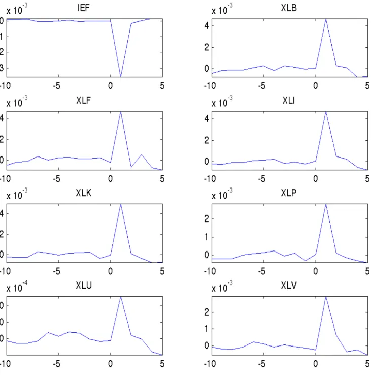
Figure 1a. Event Study for Positive NFP Surprises: Returns
Note: The event study consists of 10 5-minute periods before the release, one including the release, and 5 periods after the release.
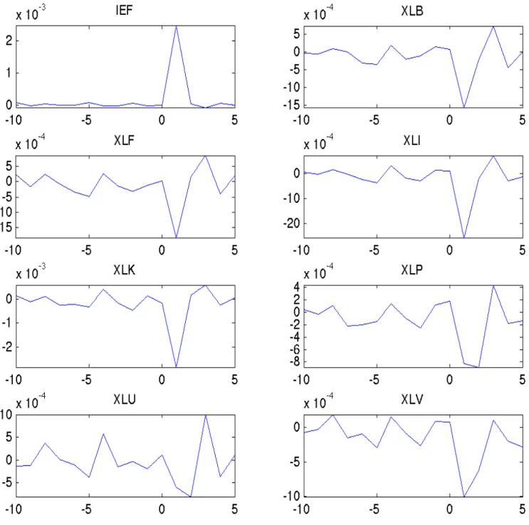
Figure 1b. Event Study for Negative NFP Surprises: Returns
Note: The event study consists of 10 5-minute periods before the release, one including the release, and 5 periods after the release.
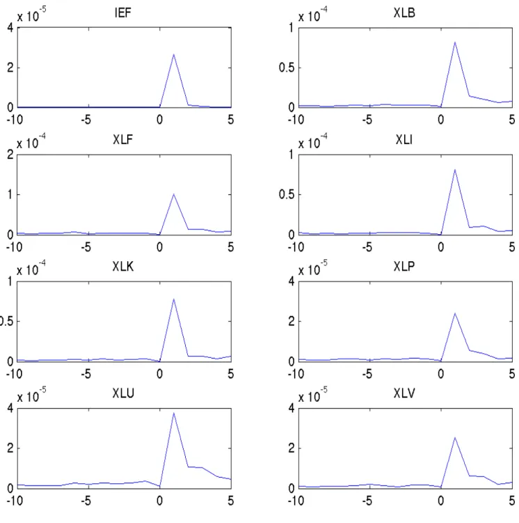
Figure 2. Event Study for Nonfarm Payrolls: Variance
The results of the event study analysis for Nonfarm Payrolls (NFP) are displayed
above in Figures 1 & 2. Figure 1 shows the average returns for each asset in 5 minute
periods around the event, separated by positive NFP surprises in Figure 1a and
neg-ative NFP surprises in Figure 1b. As you can see, NFP surprises clearly affect asset
returns, and the response is dependent on the sign of the surprise, supporting the
prior literature. Additionally, Figure 2 supports the literature suggesting that
volatil-ity spikes around macroeconomic news releases irrespective of the sign of the release.
The event study analysis provides a foundation for this study moving forward. It
sup-ports the previous literature, finding that macroeconomic news releases affect both the
mean and variance of the assets considered in this study. The following sections move
on to address how macroeconomic news affects portfolios of assets. The remainder
of this paper is organized as follows: first Section II reviews the prior literature and
explains how this study is a contribution to this literature, Section III describes the
dataset, Section IV outlines the methodology and empirical model to be used in this
study, Section V presents the results and discusses the findings, and finally Section VI
concludes.
II. Literature Review
The literature review is organized as follows. First, I discuss the effects of
macroe-conomic news releases on fixed income and equities, the two asset classes considered
in this study. I then discuss the relative importance of the different macroeconomic
releases, and finally introduce which releases are investigated in this paper.
A. Evidence Bonds Are Affected by Macroeconomic News Surprises
Balduzzi, Elton and Green (2001) use intraday bond price data and find that surprises
in economic announcements affect both prices and volatility in the U.S. government
bond market. Their research suggests that information from macroeconomic data
re-leases is incorporated into bond prices very rapidly. They find that volatility increases
Addi-tionally, they show that the same announcements that affect prices are also typically
associated with higher volatilities. For data regarding macroeconomic news releases,
they use the Money Market Services (MMS) database which gives both actual release
values and forecasted values. Balduzzi, Elton and Green (2001) also survey a literature
regarding these forecasts and find research suggesting that MMS forecasts are unbiased
except in the Industrial Production report. They also find MMS forecasts are more
accurate than forecasts from autoregressive models. My research incorporates a
simi-lar type of forecast, coming from the Bloomberg Professional Service, and should have
similar features. A more detailed analysis of these forecasts is given in Section III.
Fleming and Remolona (1997) further explore the bond market’s response to
macroe-conomic news and find that both bond prices and return volatility are significantly
affected by macroeconomic news. They also look at high frequency data, and find that
prices react almost instantaneously. Additionally, they find support for the results of
Balduzzi, Elton and Green (2001), suggesting that volatility increases can persist for
a significant amount of time after the announcement. They also discuss in depth the
microstructure of the bond market; however, this is irrelevant to my research, as I
follow the literature in using five minute returns for the high frequency data to avoid
microstructure issues. In a second study, Fleming and Remolona (1999) support their
previous work, and outline a two stage adjustment process for the Treasury market in
response to macroeconomic news. They conclude that there is a quick first stage where
prices adjust nearly instantaneously, with low volume followed by a longer second stage
with high volume and persistently higher volatility. Finally, research by Ederington and
Lee (1993) supports the claim that bond (and foreign exchange) prices and volatilities
are significantly affected by macroeconomic news events. They also find that volatility
increases may be persistent after the figures are released.
B. Evidence Equities Are Affected by Macroeconomic News Surprises
Boyd, Hu and Jagannathan (2005) cite Cambell and Mei (1993) in their claim that
the expected growth rate of dividends, and the equity risk premium. Macroeconomic
news releases can affect both the interest rate and the expected growth rate of future
dividends in conflicting directions; thus, the effect of macroeconomic news releases on
equities is more ambiguous than it is for fixed income securities. To begin with a daily
horizon, the evidence is mixed as to whether or not stocks are affected by
macroe-conomic news surprises. Schwert (1981) looks at reactions of daily stock returns to
announcement of CPI inflation. Schwert discusses several theoretical links between
inflation and stock returns. He mentions a credit channel, where unexpected inflation
helps net debtors at the expense of net creditors; a tax channel, where unexpected
inflation increases the revenues of a firm, but costs remain the same because inventory
decisions are made ahead of time thus these costs were incurred in the previous period,
and leads to a larger real tax burden for the firm; finally he discusses an expectations
channel, where inflation surprises contain information with respect to future levels of
inflation. Higher expected inflation causes nominal interest rates to rise, thus there is a
transfer of wealth from bondholders to stockholders.3 These channels are not quite as
direct as they may seem, because in practice there are additional factors in play such
as the use of long term contracts and central bank intervention from unexpected
infla-tion (Schwert, 1981). His research suggests that there is a weak negative relainfla-tionship
between inflation surprises and equity returns, and the magnitude and significance of
the relationship is not strong.
Pearce and Roley (1985) also discuss a theoretical framework for how macroeconomic
news announcements affect stock prices. They hypothesize that unexpected inflation
increases inflation expectations, which cause agents to expect tighter monetary policy
from the central bank, leading to lower stock prices via a higher discount rate. Their
research also discusses how real economic data announcements can affect stock prices.
As discussed earlier, they point out that a positive unexpected surprise in real activity
leads to expectations of larger cash flows having a positive effect on stock prices. They
3See Schwert (1981) for a detailed explanation of channels through which inflation surprises affect
also suggest that increases in real activity increases expectations of the discount rate
having a negative effect on stock prices, leading to an ambiguous overall effect on stock
prices. Pearce and Roley (1985) use daily stock data and their results are as follows.
The strongest evidence they found was that information related directly to monetary
policy significantly affects stock prices. They found a strong negative relationship
between money announcement surprises and stock prices. They also only found weak
evidence that inflation surprises affect stock prices and little evidence that surprises in
real economic activity affect stock prices. Finally, Pearce and Roley (1985) find that
it is only the unexpected or surprise component of the news releases that matters in
determining stock returns. This supports my decision to use macroeconomic surprise
values in the forecasts of return and variance, as opposed to the actual release value.
Adams, McQueen and Wood (2004) find that stocks are affected by inflation surprises
at an intraday frequency. They also survey other studies (Schwert, 1981; McQueen &
Roley, 1993; Flannery & Protopapadakis, 1996) and find mixed evidence at a daily
frequency that returns are significantly affected by inflation surprises. Additionally,
Savor and Wilson (2010) found that equities have a significantly higher Sharpe ratio
on announcement days. They expected to find higher returns on announcement days
because of the higher risk and uncertainty surrounding the macroeconomic news release.
They found that the average announcement day returns is 11.4 basis points (bps)
compared to 1.1 bps on non-announcement days implying that over 60 percent of the
cumulative annual risk premium is earned on announcement days. This suggests that
macroeconomic news releases do significantly affect stock prices in some manner.
Kim, McKenzie and Faff (2004) found that stock returns are affected only by
infla-tion surprises from the Consumer Price Index (CPI) and Producer Price Index (PPI)
reports. Additionally, they found that inflation surprises, as well as surprises in
unem-ployment and retail sales, increased stock market volatility, and this did not depend on
the sign of the surprise. The literature supports the claim that stock market returns
and volatilities are affected by scheduled macroeconomic news releases, with variables
macroe-conomic surprises seems to be weaker than in bond markets because of the opposing
forces of the discount rate and the expected future dividends. There is also evidence
that macroeconomic surprises have a greater effect on stock prices when a control for
the stage of the business cycle is included. This claim is supported further by Andersen
et al. (2007) who suggest that both stock and bond markets react to macroeconomic
news surprises, and the reaction in the bond market is much stronger than the reaction
in equities markets. Again, they suggest that equity markets only respond to surprises
in macroeconomic news after controlling for the state of the business cycle.
An overarching theme in the literature is that prior studies typically suggest that
news is incorporated into prices very rapidly, with increases in volatility following the
announcement, and the potential for volatility increases to persist. Overall, the
litera-ture focuses on individual asset classes, and fails to look at the response of a portfolio
of assets to macroeconomic news releases. This is where my research makes its
contri-bution. By looking at portfolio performance, we are able to better capture the relevant
effects that macroeconomic surprises have on typical investors, who own portfolios of
assets, not just one in particular. Additionally, there has been little research done to
try and quantify any benefits of better forecasting of these macroeconomic news events.
My research attempts to explore this by using the knowledge of the macroeconomic
surprise before it is released in generating forecasts for expected return and variance.
Additionally, it seems that generally there is little support for the claim that
macroe-conomic surprises affect equity prices at a daily frequency. This does not negate my
research; however, because the literature has shown there is an effect at an intraday
frequency, and also when the business cycle is controlled for. This paper considers both
of these circumstances either explicitly or implicitly.4
4Business cycle is controlled for implicitly when using a training period to generate the forecasts,
C. Relative Importance of Macroeconomic News Releases
There is some disagreement as to which announcements have the largest impact
on financial markets; however, the Nonfarm Payroll report is generally regarded as
the most important for individual assets by both the literature and practitioners alike.
Nikkinen et al. (2006) suggest that the employment cost index, producer and consumer
price indices, and NAPM reports are often considered measures of the whole economy
and thus are most significant in financial markets. Kim, McKenzie and Faff (2004) note
that retail sales and international trade balance also are important to a wide range of
asset classes. Following the prior literature, I use many of the macroeconomic news
releases found to be most important to financial markets including the following: the
employment report, producer price index, consumer price index, NAPM reports, retail
sales, durable goods, industrial production, capacity utilization, personal income, new
home sales, and consumer sentiment. I considered many macroeconomic releases to see
which releases have the largest impact on portfolio performance, as it may be different
from that of individual assets.
III. Data
I utilized the Center for Research in Security Prices (CRSP) database for daily ETF
prices and the Trades and Quotes database for ETF prices at a tick by tick frequency.
ETFs, which are passively managed funds that track specific indices, were used for
simplicity because they are very liquid and make it easy to form diverse portfolios
representing different sectors of a broader market index such as the S&P 500. There
should not be significant deviations from ETF price and underlying securities prices
since my analysis is restricted to times when markets are open. It is much easier to
compare sectors, asset classes, and style through ETFs than to recreate the indices
they track from their underlying constituents.
intraday frequency using five minute periods.5 I chose to include 10 periods before
the event and 5 after.6 I utilized more periods before the release and fewer after than
Andersen et al. (2007) because I am interested in forecasting returns and variances
around the release, not how assets behave after the release. A brief description of the
assets studied along with summary statistics are given below in Table 1. Additionally,
the sample correlation matrix for the high frequency stacked sample is displayed in
Table 2.7 The assets studied were chosen in an attempt to achieve diversification
across two asset classes and multiple equity sectors, including one fixed income ETF
and 7 equity ETFs representing different sectors of the S&P 500.
Table 1—Asset Descriptions & Sample Statistics
Ticker Description Mean (×10−3a) Standard Deviation (×10−3)b IEF 3-7 Year Treasury Bond Fund 0.098 0.021
XLB Materials Sector 0.455 0.372
XLF Financial Sector -0.135 0.502
XLI Industrials Sector 0.228 0.2
XLK Technology Sector 0.225 0.199
XLP Consumer Staples Sector 0.215 0.076
XLU Utilities Sector 0.256 0.136
XLV Health Care Sector 0.258 0.212
Note: Summary statistics displayed above are for the daily data.
5Andersen et al. (2007) used five-minute returns because they felt five minutes returns had the
correct balance between market microstructure effects that occur with too high of a sample frequency and blurring the results with more noise if a lower frequency was used. Using five-minute returns is common in the literature.
6Initially, using 10 periods before and 5 after and found results were robust to other settings.
7The correlations are of the high frequency stacked sample around the Nonfarm Payrolls release.
aMean of log returns.
Table 2—High Frequency Correlation Matrix: Stacked Sample
Asset IEF XLB XLF XLI XLK XLP XLU XLV
IEF 1
XLB -0.37 1
XLF -0.35 0.74 1
XLI -0.49 0.81 0.8 1
XLK -0.49 0.73 0.71 0.78 1
XLP -0.44 0.71 0.67 0.74 0.69 1
XLU -0.11 0.61 0.53 0.61 0.5 0.59 1
XLV -0.43 0.73 0.72 0.8 0.73 0.77 0.6 1
As expected, the Treasury bond fund (IEF) has the lowest variance, and is negatively
correlated with all of the other assets studied. When compared to the full sample, the
stacked sample (stacked around NFP event) correlations were much higher. This
sug-gests that asset correlations increase around macroeconomic news releases. Brenner,
Pasquariello and Subrahmanyam (2009) find that asset comovement around
macroeco-nomic news releases is dependent on the business cycle, where an expansion (recession)
leads to higher (lower) correlations around scheduled news releases. The majority of the
sample is during either a recovery or expansionary period (albeit a slow one), possibly
explaining the higher correlations in the stacked sample.
For data on macroeconomic surprise values, I utilize the Bloomberg Professional
Service (BPS). Bloomberg supplies the median survey value, the actual release value,
and the release date for data going back to 2002, and with this information it is then
straightforward to calculate the surprise values. As described in Balduzzi, Elton and
Green (2001), I use the surprise component of the macroeconomic news releases,
be-cause it is this surprise (deviation from expectations) that is the new information
intro-duced from the release. Following the literature (Balduzzi, Elton and Green, 2001), the
news component of the macroeconomic release is the surprise value in announcement
i, measured as:
whereAi is the actual value released for announcement i and Fi is the median survey value fetched from the BPS. Because the units of measurement vary across different
macroeconomic variables, the surprise is standardized by dividing each surprise (Ei)
by the standard deviation of surprises across all observations (σi) to come up with Si, the standardized surprise of announcementi.
(2) Si =
Ei σi
Notice that σi is constant; thus, this standardization procedure does not affect the significance of the estimates or the fit of estimations.8 This process allows us to compare
each macroeconomic variable, as all values are now in a standardized unit.
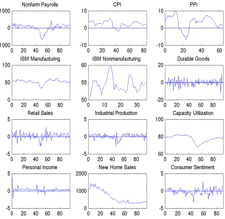
Table 3 contains the summary statistics of the macroeconomic variables that are
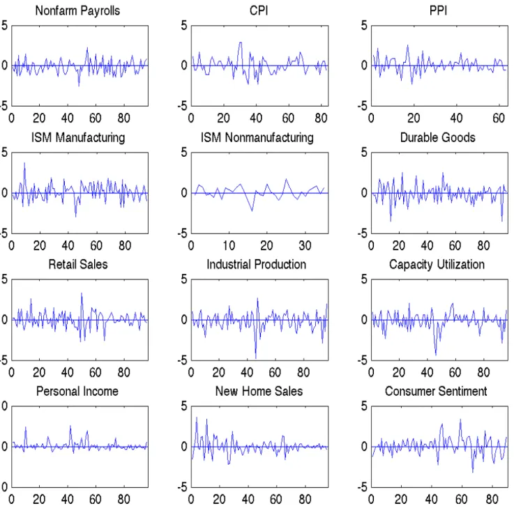
investigated in this paper. Figure 3 contains charts of actual release values over time,
Figure 4 has the standardized surprise components of each release over time, and
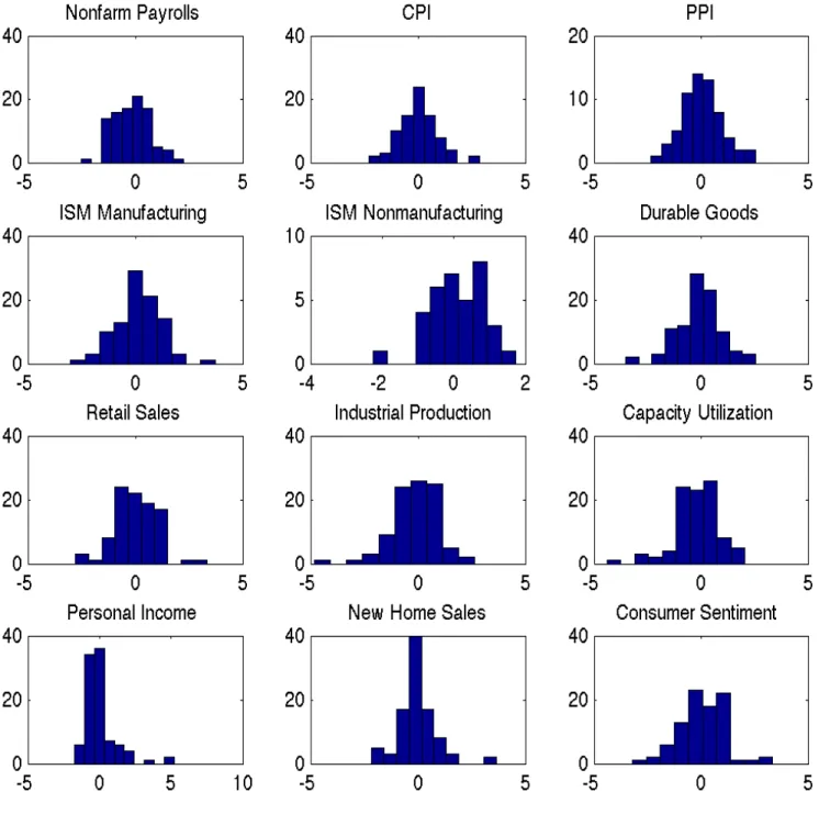
Figure 5 contains histograms of the surprise for each variable. These figures exclude
the first 24 observations in the sample because in order to forecast expected return
and variance, I used the Autoregressive (AR) and Generalized Autoregressive
Condi-tional Heteroscedasticity (GARCH) models. To estimate the parameters of the AR
and GARCH models, a training period of 24 months is used; thus, no portfolios are
actually held during the first 24 months. I will discuss the methodology in more detail
in Section IV. Additionally, it is worth noting again that my analysis occurs at a very
unique time for financial markets and the broader economy, with almost 70% of events
occurring after the beginning of the financial crisis, possibly muddying the results.
Table 3—Macroeconomic Data Release Summary Statistics.
Event Time a Sourceb Obs Date Range Meanc Act. Meand Std. Dev.e Nonfarm Payrollsf 8:30 AM BLS 131 02/2002-12/2012 -0.22 29.29 194.0
CPIg 8:30 AM BLS 107 02/2004-12/2012 0.047 2.512 1.512
PPI 8:30 AM BLS 87 10/2005-12/2012 0.072 3.423 3.482
ISM Man.h 10:00 AM ISM 131 02/2002-12/2012 0.103 53.11 5.872 ISM Non-Man.i 10:00 AM ISM 59 02/2008-12/2012 8.333 51.27 4.814 Durable Goodsj 8:30 AM BC 132 01/2002-12/2012 -0.11 0.111 3.389 Retail Salesk 8:30 AM BC 132 01/2002-12/2012 -0.00 0.259 0.905 Industrial Productionl 9:15 AM FRB 132 01/2002-12/2012 -0.15 0.137 0.654 Capacity Utilizationm 9:15 AM FRB 132 01/2002-12/2012 -0.17 77.18 3.453 Personal Incomen 8:30 AM BEA 132 01/2002-12/2012 0.138 0.336 0.505 New Home Saleso 10:00 AM BC 132 01/2002-12/2012 0.026 760.3 380.5 Consumer Sentimentp 9:55 AM MIC 113 08/2003-12/2012 0.050 0.009 0.870
Note: Some series start after 2002 because of data availability or low number of survey respondents. For most events, the average number of survey respondents was greater than 50, and the lowest average number of respondents was still greater than 20 (PPI).
aBloomberg Professional Service does not provide access to actual release times, so it was assumed
that all releases were on schedule. The number of releases that were delayed for some reason should
be immaterial to my analysis
bSources are as follows: Bureau of Labor Statistics (BLS), Institute of Supply Management (ISM),
United States Census Bureau (BC), Federal Reserve Board (FRB), Bureau of Economic Analysis
(BEA), and University of Michigan (MIC). cMean of standardized release values.
dMean of Actual Release Values.
eStandard Deviation of Actual Release Values.
fNet number of jobs added from prior month.
gYear-over-year percent change for inflation events.
hIndex level.
iIndex level.
jMonth over month percentage change in Durable Goods Orders
kMonth over month percentage change of total Retail Sales.
lMonth over month percentage change in Industrial Production.
mCapacity utilization level.
nMonth over month percentage change in Personal Income.
oSAAR of New Home Sales.
Figure 3. Actual Release Values Over Time
Figure 4. Standardized Surprises Over Time
Figure 5. Histograms of Standardized Surprise Values
As you can see in Figure 5, for the majority of releases, the median survey value
seems to be unbiased with the mean centered around 0. Additionally, the majority
of releases seem to be approximately normally distributed. This is similar to earlier
findings about survey forecasts of macroeconomic release values from MMS, suggesting
that BPS surveys are an appropriate substitute (Balduzzi, Elton and Green, 2001).
IV. Methodology & Empirical Model
Recall that in order to construct an optimal portfolio via Markowitz portfolio
op-timization, one needs forecasts for the expected returns, variances and covariances of
the assets in the universe (Markowitz, 1952). To explore the effects of perfect foresight
of macroeconomic news releases on the optimal portfolio performance, I look at how
including knowledge of the macroeconomic releases in the forecasts for expected return
and variance improves the performance of the portfolio.
I form four optimal mean-variance portfolios using different combinations of na¨ıve
and enhanced (perfect foresight included in forecast) forecasts of expected return and
variance. For tractability, I use the unconditional covariance as a na¨ıve covariance
forecast. However, this simplification may not completely mimic reality, as there is
evidence that the comovement of different asset classes is affected by macroeconomic
news releases (Brenner, Pasquariello and Subrahmanyam, 2009). With the forecasts for
expected return, variance, and covariance, I form the optimal mean-variance portfolio
using Markowitz portfolio optimization (Markowitz, 1952).910 I use the workhorse AR
(1) and GARCH (1,1) models to forecast returns and volatility respectively. Portfolio
1 is constructed with the na¨ıve forecasting methods, meaning a simple AR (1)
specifi-cation for forecasting returns, and a GARCH (1,1) for forecasting volatility. Portfolio
2 consists of a na¨ıve forecast for volatility, but utilizes an enhanced ARX (1)
specifica-tion for returns with the extra regressor being the macroeconomic surprise. Portfolio
9The risk free rate for the daily analysis was the daily return of a 30-day Treasury bill and for the
high frequency analysis, the risk free rate was numerically zero.
10Additionally, in optimal portfolio construction, portfolio weight was equal to 1 and results were
3 is constructed using a na¨ıve returns forecast and a GARCHX (1,1) volatility forecast
again, with the extra regressor being the absolute value of the macroeconomic
sur-prise value. Finally Portfolio 4 uses an enhanced forecasting method for both expected
returns and volatility. The four portfolios are summarized below in Table 4.
Table 4—Summary of Four Portfolios.
Portfolio 1 Portfolio 2 Portfolio 3 Portfolio 4 Expected Return Forecast Na¨ıve Enhanced Na¨ıve Enhanced Volatility Forecast Na¨ıve Na¨ıve Enhanced Enhanced
Daily returns are calculated from close of business the day before the macroeconomic
news release until close of business the day of the release. For the analysis at a higher
frequency, five minute returns are used.11 Judging from the event studies displayed
ear-lier, and preliminary testing using lagged surprise values, it appears that the majority
of effects of the macroeconomic news surprise were realized within 20 minutes of the
release (or market open if news was released before market opens). The hypothetical
portfolios are entered into at the end of the period before the news release, and exited
at the end of the period containing the release, meaning the portfolio is held during
the period in which the news is released. I then compare the Sharpe ratios of these
portfolios in order to see if and how knowledge of macroeconomic events affects
port-folio performance. The Sharpe Ratio is a widely used measure of risk adjusted return,
thus it is the basis for comparison of performance between the different portfolios.
The standard model for forecasting volatility is the ARCH/GARCH framework.
There is evidence in the financial literature that the GARCH volatility model does
a good job at forecasting volatility in financial markets. Hansen and Lunde (2005)
find that many extensions of GARCH (1,1) do not significantly outperform the
stan-dard GARCH (1,1) forecasts in a financial setting. The ARX (1) and GARCHX (1,1)
processes outlined below follows Bollerslev (1986) for the standard GARCH model and
expanded upon similar to Brenner, Pasquariello and Subrahmanyam (2009) who added
11I thank Dr. Michael Aguilar for giving me with code to assist in the process of culling the data
an exogenous variable in the conditional variance equation.12
(3) E[rt,i] =α0,i+α1,irt−1,i+α2,iSt+εt,i
(4) εt,i =
p
ht,iη
η∼N(0,1)
(5) ht,i = exp (β0,i+β1,i|St|) +β2,iε2t−1,i+β3,iht−1,i
where E[rt,i] is the expected return on asset i over the release period, St,i is the standardized surprise measure, εt,i is the error term and ηt,i is normally distributed with mean zero and variance of unity. The returns specification comes from a standard
AR (1) process augmented with the macroeconomic surprise. In equation (2), we have
ht,i defined above is a forecast for the magnitude of the volatility of returns. Finally, αj,i and βp,i for j = 0,1,2 and p= 0,1,2,3 are parameters to be estimated. For na¨ıve forecasts of expected return, we use the same specification, except we set α2,i = 0. Similarly, for na¨ıve volatility forecast, we set β1,i= 0. Notice the absolute value of the macroeconomic surprise |St| in the conditional variance equation (equation 5). This
follows the work of Brenner, Pasquariello and Subrahmanyam (2009) who included
the absolute value of the surprise in the conditional variance equation. Using the
absolute value also makes intuitive economic sense as well, as one would suspect the
occurrence of a surprise to increase the conditional volatility, irrespective of the sign of
the surprise. The results of Kim, McKenzie and Faff (2004) supported this intuition.
One potential explanation could be that as uncertainty is resolved by the introduction
12I use a training period before each event to fit the GARCHX model and then create the forecast
of new information, heterogenous agents’ differing interpretations of the news leads to
higher volatility. This explanation is similar to the work by Ross (1989) who found
that simply the introduction of new information increased volatility.
Additionally, portfolio optimization requires a forecast for covariance. As stated
earlier, I use the unconditional covariances to forecast the covariance between assets,
and only explore if perfect forecasting improves portfolio performance through the
channels of expected return and volatility. More formally, the variance/covariance
matrix (Σt) used to generate the optimal portfolio weights will be generated as follows:
(6) Σt =
ht,1 σ1,2 · · · σ1,n σ2,1 ht,2 · · · σ2,n ... ... ... ... σn,1 σn,2 · · · ht,n
whereht,i is the forecasted variance from the GARCHX (1,1) process for assetiin time
t, and σi,j is the unconditional covariance of returns of assets i and j.13
Once I have constructed the portfolio Sharpe ratios (average excess returns divided
by standard deviation of returns), all that remains is to test to see if perfect forecasting
significantly improves the Sharpe ratio. The first statistical test of Sharpe Ratios was
developed by Jobson and Korkie (1981). Ledoit and Wolf (2008) improved upon the
original tests and I follow their methodology to formally test for differences in Sharpe
Ratios.14
V. Results & Comparison to Literature
My analysis reveals that, contrary to my apriori, there was little effect of adding
the knowledge of the macroeconomic surprise before it was released on portfolio
per-formance. In Table 5 below, you can see the Sharpe Ratios of each portfolio for the
13For robustness, I did vary certain parameters of my analysis, such as the number of periods before
and after an event when stacking the data and the length of the training period. My results were qualitatively similar to the original analysis.
14Ledoit and Wolf (2008) published their MATLAB code for their Statistical tests of Sharpe Ratios
daily data. Table 6 displays the Sharpe Ratios for the high frequency data. The tables
following show the components of the Sharpe ratio for each portfolio, the average
ex-cess return and standard deviation.15 Additionally, Figure 6 displays the cumulative
returns for each event for the daily analysis. Figures 7 displays the same material,
except for the high frequency analysis.
While there is some improvement in the Sharpe Ratio of enhanced portfolios in
certain events, on balance it appears that there is little evidence to support the claim
that knowledge of the macroeconomic news release improves portfolio performance.
The Ledoit and Wolf (2008) statistical test of Sharpe Ratios also showed that none
of the outperformances were significantly different from the na¨ıve portfolio at the 5%
level. This is likely because in most cases, it seems to be a few key events where the
portfolio returns separate from each other, and the rest of the days, the four portfolios
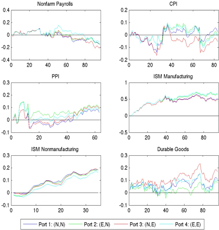
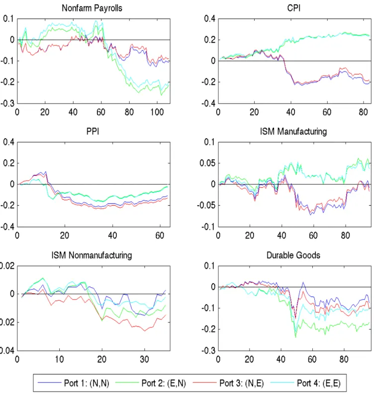
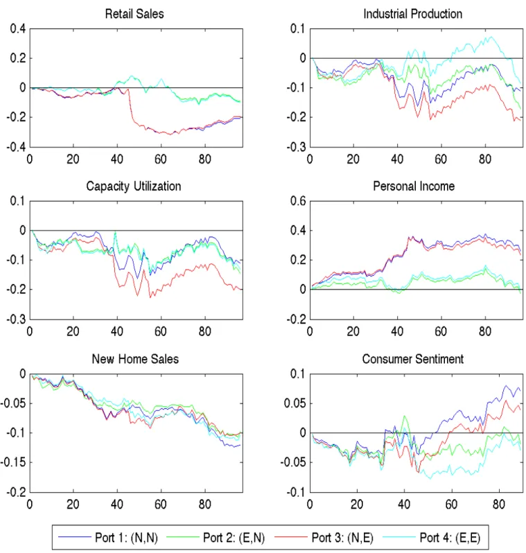
moved more or less in line with one another. This is also illustrated in Figures 8 & 9,
which plots the spread of each portfolio over Portfolio 1 for each event (not cumulative).
Notice how there are large spikes for certain days, which determines the final relative
performance for the portfolio. There does not seem to be any trend or extended periods
of successful outperformance by the enhanced portfolios. These observations hold for
the analysis at a higher frequency as well, although to a lesser extent. As seen in Figure
9, there are some sustained periods of outperformance by enhanced portfolios in the
CPI, PPI, ISM Nonmanufacturing, and Retail Sales reports.
15For high frequency data average excess return equaled average return because the risk free rate
Table 5—Sharpe Ratios: Daily Data
Port 1 Port 2 Port 3 Port 4 Nonfarm Payrolls -0.068 -0.071 -0.095 -0.052
CPI 0.013 0.001 -0.024 -0.005
PPI 0.036 0.051 0.052 0.04
ISM Manufacturing 0.173 0.23 0.169 0.239 ISM Nonmanufacturing 0.5 0.469 0.44 0.414 Durable Goods 0.059 0.043 0.087 0.044 Retail Sales -0.046 -0.046 -0.087 -0.085 Industrial Production 0.025 0.011 0.002 -0.017 Capacity Utilization 0.025 -0.008 0.001 -0.054 Personal Income -0.096 -0.059 -0.106 -0.086 New Home Sales 0.042 0.029 0.195 0.125 Consumer Sentiment 0.113 0.114 0.078 0.108
Table 6—Sharpe Ratios: High Frequency Data
Port 1 Port 2 Port 3 Port 4 Nonfarm Payrolls -0.065 -0.118 -0.055 -0.112
CPI -0.124 0.207* -0.101 0.178*
PPI -0.085 -0.017 -0.101 -0.022
ISM Manufacturing -0.008 0.052 -0.018 0.041 ISM Nonmanufacturing 0.017 -0.056 -0.133 -0.02 Durable Goods -0.045 -0.105 -0.065 -0.06 Retail Sales -0.123 -0.072 -0.115 -0.075 Industrial Production -0.077 -0.113 -0.131 -0.056 Capacity Utilization -0.077 -0.093 -0.128 -0.084 Personal Income 0.151 -0.016 0.133 -0.001 New Home Sales -0.267 -0.227 -0.192 -0.212 Consumer Sentiment 0.082 -0.022 0.043 -0.035
Table 7—Portfolio Standard Deviation: Daily Data
Port 1 Port 2 Port 3 Port 4 Nonfarm Payrolls 0.022 0.022 0.023 0.023
CPI 0.027 0.026 0.026 0.027
PPI 0.027 0.029 0.027 0.029
ISM Manufacturing 0.03 0.029 0.03 0.029 ISM Nonmanufacturing 0.011 0.011 0.012 0.011 Durable Goods 0.019 0.019 0.02 0.021 Retail Sales 0.026 0.025 0.027 0.024 Industrial Production 0.02 0.018 0.023 0.024 Capacity Utilization 0.02 0.019 0.022 0.024 Personal Income 0.029 0.028 0.032 0.032 New Home Sales 0.02 0.019 0.023 0.021 Consumer Sentiment 0.029 0.031 0.035 0.033
Table 8—Portfolio Standard Deviation: High Frequency Data
Port 1 Port 2 Port 3 Port 4 Nonfarm Payrolls 0.015 0.017 0.015 0.017
CPI 0.021 0.014*** 0.022 0.016***
PPI 0.021 0.019 0.02 0.019
ISM Manufacturing 0.01 0.009 0.009 0.009 ISM Nonmanufacturing 0.004 0.004 0.003** 0.003** Durable Goods 0.017 0.017 0.017 0.017 Retail Sales 0.018 0.013 0.018 0.014 Industrial Production 0.015 0.016 0.017 0.016 Capacity Utilization 0.015 0.016 0.016 0.016 Personal Income 0.018 0.015 0.018 0.015 New Home Sales 0.005 0.005* 0.005 0.005* Consumer Sentiment 0.01 0.009 0.01 0.009
Table 9—Average Return: Daily Data
Port 1 Port 2 Port 3 Port 4 Nonfarm Payrolls -0.002 -0.002 -0.002 -0.001
CPI 0 0 -0.001 0
PPI 0.001 0.001 0.001 0.001
ISM Manufacturing 0.005 0.007 0.005 0.007 ISM Nonmanufacturing 0.005 0.005 0.005 0.005 Durable Goods 0.001 0.001 0.002 0.001 Retail Sales -0.001 -0.001 -0.002 -0.002 Industrial Production 0.001 0 0 0 Capacity Utilization 0.001 0 0 -0.001 Personal Income -0.003 -0.002 -0.003 -0.003 New Home Sales 0.001 0.001 0.004 0.003 Consumer Sentiment 0.003 0.004 0.003 0.004
Table 10—Average Return: High Frequency Data
Port 1 Port 2 Port 3 Port 4 Nonfarm Payrolls -0.001 -0.002 -0.001 -0.002
CPI -0.003 0.003** -0.002 0.003**
PPI -0.002 0 -0.002 0
ISM Manufacturing 0 0 0 0
ISM Nonmanufacturing 0 0 0 0
Durable Goods -0.001 -0.002 -0.001 -0.001 Retail Sales -0.002 -0.001 -0.002 -0.001 Industrial Production -0.001 -0.002 -0.002 -0.001 Capacity Utilization -0.001 -0.002 -0.002 -0.001
Personal Income 0.003 0 0.002 0
New Home Sales -0.001 -0.001 -0.001 -0.001
Consumer Sentiment 0.001 0 0 0
Table 11—Percent Outperforming Portfolio 1: Daily
Port 2 Port 3 Port 4 Nonfarm Payrolls 39.6 29.2 42.7
CPI 37.3 24.1 36.1
PPI 33.3 25.4 30.2
ISM Manufacturing 42.1 21.1 44.2 ISM Nonmanufacturing 54.3 57.1 54.3
Durable Goods 43.8 52.1 51
Retail Sales 41.7 24 40.6
Industrial Production 41.7 33.3 45.8 Capacity Utilization 47.9 42.7 49 Personal Income 47.9 45.8 47.9 New Home Sales 50.5 61.1 62.1 Consumer Sentiment 50.6 24.7 44.9
Table 12—Percent Outperforming Portfolio 1: High Frequency
Port 2 Port 3 Port 4 Nonfarm Payrolls 41.7 17.6 40.7
CPI 62.7 24.1 59
PPI 47.6 4.8 47.6
ISM Manufacturing 51.6 36.8 52.6 ISM Nonmanufacturing 48.6 31.4 48.6
Durable Goods 50 12.5 49
Retail Sales 46.9 9.4 47.9
Industrial Production 50 14.6 57.3 Capacity Utilization 49 15.6 49 Personal Income 45.8 28.1 44.8
New Home Sales 51 31.3 49
Figure 6a. Cumulative Returns: Daily Data
Figure 6b. Cumulative Returns: Daily Data
Figure 7a. Cumulative Returns: High Frequency Data
Figure 7b. Cumulative Returns: High Frequency Data
Figure 8a. Event by Event Spread Over Portfolio 1: Daily Data
Figure 8b. Event by Event Spread Over Portfolio 1: Daily Data
Figure 9a. Event by Event Spread Over Portfolio 1: High Frequency
Figure 9b. Event by Event Spread Over Portfolio 1: High Frequency
Admittedly, my initial hypothesis was rejected, and there is no doubt this requires
significant discussion in itself. Before that question is addressed; however, I first point
out some interesting themes present in the results. First, the way in which the enhanced
portfolios behaved was quite interesting. For the high frequency analysis, Portfolio 1
and Portfolio 3 generally tracked each other rather closely. Similarly, Portfolio 2 and
Portfolio 4 followed each other very closely as well. This implies that the additional
news from a macroeconomic surprise is included into the portfolio weights through an
expected return channel rather than a volatility channel. This is further supported in
the components of the Sharpe Ratios presented in tables 8 and 10. Notice that the
three events with the strongest outperformance (CPI, PPI, and Retail Sales) all have
higher returns and lower variances in Portfolio 2 vs. Portfolio 3, suggesting that the
main contributor to Portfolio 4’s success was the additional information in the return
forecasts rather than the volatility forecasts.
Additionally, by qualitatively looking at the cumulative performances of each
port-folio, it is interesting that two of the four cases of sustained outperformance were in
inflation events (CPI and PPI). Although it is still an insignificant outperformance
according to the Ledoit and Wolf (2008) test at the 5% level (but CPI is significant
at 10% level), there is evidence in the literature that suggests inflation surprises
af-fect equity prices more than surprises regarding real economic activity. Focusing just
on the portfolio return in the high frequency analysis, Portfolios 2 and 4 had a
sig-nificantly higher mean return than Portfolio 1 for the CPI event, further supporting
the claim that inflation surprises affect stocks more than surprises in real economic
variables. Additionally, Table 8 shows that Portfolios 2 & 4 in the CPI event had a
significantly lower standard deviation than the na¨ıve portfolio, further contributing to
its success. Tables 11 and 12 show the percentages of events with a higher return than
the corresponding return of Portfolio 1. Notice the numbers are rarely above 50%, and
only the CPI (High Frequency) and New Home Sales (Daily) have an outperformance
more than 60% of the time for at least one portfolio. This qualitative analysis
equities than surprises in real economic variables. Additionally, the inflation surprises
performed better in the high frequency analysis than for the daily frequency
analy-sis, further supporting the literature that says financial markets are more significantly
affected by macroeconomic surprises at an intraday frequency versus a daily frequency.
Now that the results have been presented, we must ask the question of why did the
majority of portfolios not perform as our initial hypothesis would suggest? To begin,
it must be noted, as stated multiple times, that the time period studied was a very
unique period for financial markets. Many in the financial press have suggested that
the financial crisis and the policy responses to the crisis have altered the way that
markets accept macroeconomic news during the latter portion of the period studied.
Recall my dataset covered the periods of January 2002 - December 2012. When the
two year training period is taken out of this, the dates the hypothetical portfolios are
actually held are all within the period January 2005 - December 2012, meaning that
almost 70% of these portfolios are held during or after the financial crisis began in mid
2007.
Some of the reasons for this strange time for financial markets are the actions taken by
the Federal Reserve (Fed). The three rounds of Large Scale Asset Purchases (LSAPs),
or more commonly Quantitative Easing (QE), have had a huge impact on financial
markets. LSAPs introduce tremendous amounts of liquidity into financial markets,
and many have hypothesized that this liquidity has been a cause of the bull market in
equities since the bottoms of the recession in 2009, especially as the overall economy
has been slow to recover, with lackluster growth and persistently high unemployment.
This would imply that financial markets have lost touch with the underlying economic
fundamentals and the way in which these markets interpret economic information would
necessarily be altered. Additionally, the traditional policy tool for the Fed, the Federal
Funds Rate (FFR), has been at the zero lower bound since late 2008. There are
numerous other policies, such as the Maturity Extension Program (Operation Twist)
and different forward guidance strategies that have also affected financial markets in an
all these policies is they attempt to put downward pressure on longer term interest
rates, in an effort to move people out the risk spectrum into more risky assets, thus
stimulating the economy through various channels. The question of how this affects
financial markets and their interpretation of macroeconomic news is quite complicated
and there is little research in the area. But one way in which these policies could
muddy the results presented earlier is that financial markets could be focused more
on the liquidity provided by the Fed than the underlying economic fundamentals.
For example, depending on the market sentiment regarding Fed actions, markets may
interpret good news about the economy as signal for future Fed actions, rather than
the underlying fundamentals of the economy. This is a similar idea to that proposed
by Boyd, Hu and Jagannathan (2005) who find that bad news is typically good news
for stocks in good times, and bad during contractions. This stems from the conflicting
affects of economic news on the expected future cash flows and discount rate. It is
quite possible that financial markets are more focused on the discount rate and actions
by the Fed than the underlying economic fundamentals. In this unprecedented time
of monetary stimulus, markets may quickly change their expectations for future Fed
actions, thus their responses to additional macroeconomic news may change over time.
Another potential reason that my apriori was incorrect could be the lack of
diversi-fication of assets studied. As stated earlier, I only studied 8 assets, including 7 sector
specific equity ETFs and one U.S. Treasury ETF. Because the equity ETFs are so
highly correlated, it is likely they behave similarly to macroeconomic news surprises,
meaning their forecasts for expected return and variance would also behave similarly,
possibly mitigating the differences in weights of the enhanced versus the na¨ıve
portfo-lios. The prior literature overwhelmingly supports the claim that bond markets were
much more strongly affected by macroeconomic surprises than equities, so having a
large number of equity ETFs could be simply adding noise to my results.
A final possible reason for the lack of significant effect could be the frequency studied.
Because the price response to macroeconomic news occurs almost instantaneously, the
the portfolios were exited twenty minutes after the release or market open if the news
was released before the market opens. This was to be sure to capture the increases in
volatility around the macroeconomic news releases (since evidence suggested volatility
increases can persist after macroeconomic news releases); however, the results showed
that the macroeconomic news affected the enhanced portfolios through an expected
re-turn channel rather than a variance channel. For this reason, the windows in which the
portfolios are held may have been too large, meaning the effects of the macroeconomic
news release on the mean price response were not captured.
VI. Conclusion
The evidence presented in this paper suggests that although macroeconomic news
events affect individual assets returns and variances, when this information is
aggre-gated into a portfolio of assets, the ex ante knowledge of the release value does not
improve the performance of the portfolio. This could be a result of the time period
studied, including the financial crisis, the lack of diversity of assets studied or the
sample frequency used in the high frequency analysis. Future research should include
additional asset classes with more diversification and different time periods to better
address these issues. Future research could also consider sampling at a higher frequency,
REFERENCES
Adams, Greg, Grant Richard McQueen, and Robert Wood.2004. “The Effects of Inflation News on High Frequency Stock Returns.” Journal of Business.
Andersen, Torben G., Tim Bollerslev, Francis X. Diebold, and Clara Vega.
2007. “Real-Time Price Discovery In Global Stock, Bond and Foreign Exchange Markets.” Journal of International Economics, 73: 251–277.
Balduzzi, Pierluigi, Edwin J. Elton, and T. Clifton Green. 2001. “Economic News and Bond Prices: Evidence from the U.S. Treasury Market.” Journal of Fi-nancial and Quantitative Analysis, 523–543.
Bollerslev, Tim.1986. “Generalized Autoregressive Conditional Heteroskedasticity.”
Journal of Econometrics, 31(3): 307–327.
Boyd, John H., Jian Hu, and Ravi Jagannathan. 2005. “The Stock Market’s Reaction to Unemployment News: Why Bad News is Usually Good for Stocks.”The
Journal of Finance, 60(2): 649–672.
Brenner, Menachem, Paolo Pasquariello, and Marti Subrahmanyam. 2009. “On the Volatility and Comovement of U.S. Financial Markets around Macroe-conomic News Announcements.” Journal of Financial and Quantitative Analysis, 44(6): 1265–1289.
Cambell, J.Y., and J. Mei. 1993. “Where Do Betas Come From? Asset Price Dy-namics and the Source of Systemic Risk.”The Review of Financial Studies, 6(3): 567– 592.
Ederington, Louis H., and Jae Ha Lee.1993. “How Markets Process Information: News Releases and Volatility.” The Journal of Finance, 48(4): 1161–1191.
Fleming, Michael J., and Eli M. Remolona.1997. “What Moves the Bond Mar-ket?” Economic Policy Review, 3(4).
Hansen, Peter R., and Asger Lunde. 2005. “A Forecast Comparison of Volatility Models: Does Anything Beat a GARCH (1,1)?” Journal of Applied Econometrics, 20(7): 873–889.
Jobson, J.D., and Bob M. Korkie. 1981. “Performance Hypothesis Testing with the Sharpe and Treynor Measures.” The Journal of Finance, 36(4): 889–908.
Kim, Suk-Joong, Michael D. McKenzie, and Robert W. Faff. 2004. “Macroe-conomic News Announcements and the Role of Expectations: Evidence for US Bond, Stock and Foreign Exchange Markets.” Journal of Multinational Financial
Manage-ment, 14(4): 217–232.
Ledoit, Olive, and Michael Wolf. 2008. “Robust Performance Hypothesis Testing with the Sharpe Ratio.” Journal of Empirical Finance, 15(5): 850–859.
Markowitz, Harry.1952. “Portolio Selection.” The Journal of Finance, 7: 77–91.
Nikkinen, Jussi, Mohammed Omran, Petri Sahlstrom, and Janne Aijo.2006. “Global Stock Market Reactions to Scheduled U.S. Macroeconomic News Announce-ments.” Global Finance Journal, 17(1): 92–104.
Pearce, Douglas K., and V. Vance Roley. 1985. “Stock Prices and Economic News.” The Journal of Business, 58(1).
Ribeiro, Ruy, and Pietro Veronesi. 2002. “The Excess Comovement of Interna-tional Stock Markets in Bad Times.” Working Paper.
Ross, Stephen A. 1989. “Information and Volatility: The No-Arbitrage Martingale Approach to Timing and Resolution Irrelevancy.”The Journal of Finance, 44(1): 1– 17.
Savor, Pavel, and Mungo Wilson. 2010. “How Much do Investors Care about Macroeconomic Risk? Evidence from Scheduled Economic Announcements.” Work-ing Paper.