DOI:10.1051/ps/2017018 www.esaim-ps.org
SMALL AND LARGE SCALE BEHAVIOR OF MOMENTS OF POISSON
CLUSTER PROCESSES
Nelson Antunes
1, Vladas Pipiras
2, Patrice Abry
3and Darryl Veitch
4Abstract. Poisson cluster processes are special point processes that find use in modeling Internet traffic, neural spike trains, computer failure times and other real-life phenomena. The focus of this work is on the various moments and cumulants of Poisson cluster processes, and specifically on their behavior at small and large scales. Under suitable assumptions motivated by the multiscale behavior of Internet traffic, it is shown that all these various quantities satisfy scale free (scaling) relations at both small and large scales. Only some of these relations turn out to carry information about salient model parameters of interest, and consequently can be used in the inference of the scaling behavior of Poisson cluster processes. At large scales, the derived results complement those available in the literature on the distributional convergence of normalized Poisson cluster processes, and also bring forward a more practical interpretation of the so-called slow and fast growth regimes. Finally, the results are applied to a real data trace from Internet traffic.
Mathematics Subject Classification. 60G55, 60G18, 60K30, 60G22.
Received November 24, 2016. Accepted September 27, 2017.
1. Introduction
A Poisson cluster process (PCP, for short; sometimes also called cluster Poisson process or CPP) consists of points usually defined on the positive half-axis (0,∞) whose positions are determined by the following construction. Clusters of a finite number of points are assumed to arrive according to a Poisson arrival process with intensityλ >0 at times Sj, j≥1 (with 0< S1< S2< . . .). The clusters are i.i.d. copies with a random
but almost surely finite number of pointsWj. The focus throughout is on clusters having the following structure:
the Wj points are separated in time by i.i.d. sequence of positive interarrival timesAj,k, k ≥1, and the first
point of a cluster is located at the arrival time of the cluster. Such PCPs are also known as the Bartlett–Lewis processes after Bartlett [4] and Lewis [23] (see, for example, Cox and Isham [6], Daley and Vere–Jones [7]).
Keywords and phrases. Poisson cluster process, scaling, moments, cumulants, heavy tails, slow growth regime, fast growth regime, Internet traffic modeling.
1 Center for Computational and Stochastic Mathematics, University of Lisbon, and University of Algarve, Campus de Gambelas, 8005–139 Faro, [email protected]
2 Department of Statistics and Operations Research, University of North Carolina, CB 3260, Chapel Hill, NC 27599, USA.
3 Univ Lyon, Ens de Lyon, Univ Claude Bernard, CNRS, Laboratoire de Physique, 69342 Lyon, France.
4 School of Computing and Communications, University of Technology Sydney, P.O. Box 123, Broadway, NSW 2007, Australia.
ET AL.
In mathematical terms, ifN(B) denotes the number of such PCP points in a setB⊂(0,∞), then
N(B) =
∞
j=1
Wj−1
k=0
1B
Sj+
k
m=1
Aj,m
, (1.1)
where 1B(x) is the indicator function of the set B. The PCP N defined by (1.1) is called transient(that is, nonstationary), since the distributions ofN(B) andN(B+T) are in general not equal forT >0 andB⊂(0,∞), whereB+T ={x+T :x∈B}. TheequilibriumPCPNe(B) is defined asN(B+T) lettingT → ∞. For the
equilibrium process, the distributions ofNe(B) andNe(B+h) are the same for anyh >0 andB⊂(0,∞). The
equilibrium processNecan be viewed as stationary, and will be the focus throughout this work.
PCPs form an interesting class of point processes which has been studied in theory (e.g. in the general context of point process; see Cox and Isham [6], Karr [20], Daley and Vere–Jones [7]) and used successfully in applications (e.g. computer failure patterns in Lewis [23], software reliability in Zeephongsekulet al. [36], neural spike trains in Gr¨uneis et al.[14,15], physics in Saleh and Teich [31], Lowen and Teich [24], rainfall in Onof et al. [28]). The motivating application in this work is the Internet traffic observed on a network link, where points are data packets and clusters are packet flows (essentially packetized document files, web pages, videos or other application contents). The use of PCPs in modeling data packet traffic was popularized by Hohn
et al.[18], see also Fa¨yet al.[11], Mikosch and Samorodnitsky [27], Fasen and Samorodnitsky [10], Gonz´ alez-Ar´evalo and Roy [13], Antunes and Pipiras [3]. Models related to PCPs for modeling Internet traffic include the ON/OFF model (e.g.Lelandet al.[22]), the infinite source Poisson arrival process (e.g.Mikoschet al.[26], Guerinet al.[16]), and the renewal point process (e.g.Kaj [19], Gaigalas and Kaj [12]).
In this work, we focus on the moments and cumulants of PCPs. On the one hand, moments and cumulants are among the most basic and fundamental quantities of any random object of study and, in fact, have already been studied for PCPs to some extent (see references in Sect.2 below). We are particularly interested here in their scaling behavior at large (coarse) and small (fine) scales, especially in connection to the use of PCP models motivated by the “self-similar” and multiscale nature of Internet traffic (e.g.Abryet al.[1], Hohnet al.[18]).
More specifically, we will consider the following moments of PCPs: for integerr≥1,
(usual) moments :mr(a) =ENe(0, a)r, (1.2)
factorial moments :m[r](a) =ENe(0, a)[r], (1.3)
central moments :m0r(a) =E(Ne(0, a)−ENe(0, a))r, (1.4)
wheren[r]=n(n−1). . .(n−r+ 1) for a nonnegative integernanda >0 will be referred to as “scale.” Central moments are natural to consider in view of some of the large scale limiting results available for centered PCPs (see (5.15) and (5.16) below). Factorial moments are considered because, as will be shown, they may be more informative about PCPs than the usual or central moments.
The quantities most convenient to work with in the context of PCPs are not any of the moments above but rather factorial cumulants. Moreover, the (usual) cumulants are often considered in practice, in addition to the (usual) moments. We will thus also consider: for integerr≥1,
(usual) cumulants :κr(a) =
∂rlogM a(t)
∂tr
t=0, (1.5)
factorial cumulants :κ[r](a) =
∂rlogPa(z)
∂zr
z=1, (1.6)
where Pa(z) is the probability generating function of the equilibrium PCP on the interval (0, a) (see Sect. 2
for definition) and Ma(t) is the moment generating function of the equilibrium PCP on the interval (0, a). In fact, the results of interest will be derived first for factorial cumulantsκ[r](a) and then used to obtain analogous
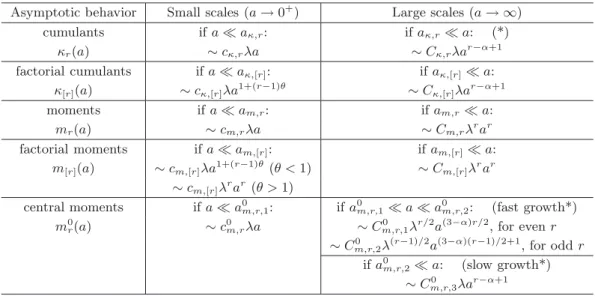
Table 1. The asymptotic behavior of the various moments and cumulants (r≥2).
Asymptotic behavior Small scales (a→0+) Large scales (a→ ∞)
cumulants ifaaκ,r: ifaκ,ra: (*)
κr(a) ∼cκ,rλa ∼Cκ,rλar−α+1
factorial cumulants ifaaκ,[r]: ifaκ,[r]a:
κ[r](a) ∼cκ,[r]λa1+(r−1)θ ∼Cκ,[r]λar−α+1
moments ifaam,r: ifam,r a:
mr(a) ∼cm,rλa ∼Cm,rλrar
factorial moments ifaam,[r]: ifam,[r]a:
m[r](a) ∼cm,[r]λa1+(r−1)θ (θ <1) ∼Cm,[r]λrar ∼cm,[r]λrar (θ >1)
central moments ifaa0m,r,1: ifa0m,r,1aa0m,r,2: (fast growth*)
m0
r(a) ∼c0m,rλa ∼Cm,r,0 1λr/2a(3−α)r/2, for evenr ∼C0
m,r,2λ(r−1)/2a(3−α)(r−1)/2+1, for oddr ifa0m,r,2a: (slow growth*)
∼C0
m,r,3λar−α+1
Small and large scale behaviors of the quantities (1.2)–(1.4) and (1.5)–(1.6) refer, respectively, to a → 0+ and a → ∞. As indicated above, in connection to Internet traffic and especially its self-similar (multiscale) nature, it has become common and useful to examine various quantities as analysis scale changes. In our study, we shall make the following assumptions motivated by the applications to Internet traffic. At large scales (a → ∞), we shall assume, in particular, that the cluster size distribution of W = Wj is heavy–tailed with
exponentα∈(1,2) in the sense that
P(W > w)∼CWw−α, as w→ ∞, (1.7)
where ∼denotes the asymptotic equivalence andCW >0 is a constant. This is a common assumption in the
Internet traffic models, based on empirical findings (e.g. Abry et al. [2]). At small scales (a → 0+), we shall assume that the cumulative distributionF of interarrival timesA=Aj,m has a densityf satisfying: forθ > 0
andCf >0,
f(t)∼Cftθ−1, as t→0+. (1.8)
In the applications to Internet traffic, F is often taken as a gamma distribution, that satisfies (1.8). For the Internet traffic data considered in this work, the parameter θ of the gamma distribution satisfying (1.8) is estimated to be smaller than 1.
Under the assumptions (1.7) and (1.8), the asymptotic behavior of the various cumulants and moments at small and large scales is summarized in Table1forr≥2. In each case, the asymptotic behavior is expressed in terms ofλanda, and a constant which depend only onr, and possibly the distributions ofW (at large scales) and A (at small scales), with the exception of the factorial moments at small scales when θ = 1. The latter case is not included in the table but is treated in our analysis below. We also specify the scales for which the asymptotic results are expected to hold in practice:e.g. aaκ,r andaκ,rafor cumulants whereaκ,r is the
transition scale between small and large scales obtained by equating the two asymptotic behaviors at small and large scales, and solving fora. (The notation stands for the heuristic “much smaller.”) The exact forms of all the constants and transition scales will be given below.
ET AL.
distinguishes between the so–called fast growth regime corresponding to large λ/aα−1 and the slow growth
regime corresponding to small λ/aα−1 (see Sect. 5 for more information). The different asymptotic behaviors
of the central moments at large scales in Table1 correspond to these two regimes. We should stress that all the other stated results at large scales are valid in both slow and fast growth regimes. We also note that the results indicated by (*) in Table 1, have been verified up to the order r= 10 only but otherwise conjectured to hold for allr.
Several interesting conclusions can be drawn from Table 1. For example, on the moments side and at large scales, note that the exponentα in (1.7) is captured by the central moments only, while at small scales, the exponent θ in (1.8) is captured by the factorial moments and in the case θ <1 only. The factorial cumulants, on the other hand, have the exponentsαandθ at large and small scales, respectively. One natural interest in the obtained scaling relations is that they could be used for robust estimation procedures while inferring the scaling behavior. Our results for the central moments at large scales provide a more practical interpretation of the slow and fast growth regimes. Indeed, as argued below, these regimes reflect naturally the changing nature of the central moments as aincreases for fixed λ; whereas in the earlier literature, λwas associated with the length of the time window where the PCP was observed.
Our results on the large scale asymptotic behavior of the various moments are closest in the spirit to those of Dombry and Kaj [9] who considered moment measures in the parallel context of renewal point processes. But it should be noted that our approach and proofs are different, and some of the issues considered here are not addressed in Dombry and Kaj [9]. Further comparison with the work of Dombry and Kaj [9] will be provided (see Rem.5.3below).
Our results at small scales are somewhat connected to the so-called multifractal analysis which similarly focuses on the scaling behavior of the usual moments and cumulants of various quantities at small scales (e.g.
Wendtet al.[33]). We shall pursue these connections in greater detail elsewhere. But we would like to note here that the behavior of PCPs and related models in connection to Internet traffic and multifractals, was explored in Hohn et al.[18], Veitch et al. [32], Ribeiro et al. [30], Krishnaet al. [21]. The use of factorial moments in the multifractal (intermittency) analysis of point process data, instead of the usual moments, can be found in Carrutherset al.[5], de Wolfet al.[8], in connection to high-energy multiparticle collisions.
In summary, the structure of the paper is as follows. In Section 2, we provide the known formulae for the various cumulants and moments of PCPs. The behavior of the moments of PCP at large scales is studied in Section 3. Section 4 concerns the behavior of the moments at small scales. The large scale behavior in the slow and fast regimes mentioned above is discussed in Section 5. The transition between the different scaling behaviors is discussed in Section 6. The application to Internet traffic is given in Section7, where we find the various empirical moments of the Internet traffic data set to be described quite well by the derived formulae for the moments of PCP and their asymptotic relations. Finally, in AppendixA, we provide the formulae relating the first 7 central moments and factorial cumulants, which are used in Section5, and in AppendixB, we derive the formulae for the factorial cumulants of PCP, adapting the approach of Westcott [34].
2. Moments and cumulants of Poisson cluster processes
The definition of moments and cumulants and their relations for general point processes are given in Daley and Vere–Jones [7] (Sect. 5.2). We gather here these formulae for the Poisson cluster processes (PCPs). We also introduce some notation used throughout this work. The focus is on the PCP N given by (1.1), and the corresponding equilibrium PCPNediscussed following (1.1).
The interarrival timesAj,min (1.1) between the points in a cluster are independent and identically distributed
as a random variableAhaving distribution function
Itskth convolution will be denotedFk,k≥1, withF1=F. The numbers of pointsWjin clusters are independent
and identically distributed as a random variableW with probability mass function
pW(w) =P(W =w), w≥1. (2.2)
Its tail probability will be denoted
Rw=P(W ≥w), w≥1. (2.3)
As in (1.1), the starting pointsSj of the clusters are the arrival times of a Poisson process with intensityλ >0.
Let
Pt(z) =EzNe(0,t) (2.4)
be the probability generating function of the equilibrium PCP on the interval (0, t). Factorial cumulants
ofNe(0, t) are defined as
κ[r](t) = ∂
rlogP t(z)
∂zr
z=1, r≥1. (2.5)
The factorial cumulants of the equilibrium PCPNe can also be obtained as
κ[1](t) =λEW t, κ[2](t) = 2λ ∞
k=1
t
0 Fk(u)du
∞
j=1
Rj+k (2.6)
and, forr >2,
κ[r](t) = (r−1)rλ
∞
k=r−1
(k−1)(k−2). . .(k−r+ 2)
t
0 Fk(u)du
∞
j=1
Rj+k. (2.7)
The formulas (2.6)–(2.7) appear in Westcott [34] when the first points of the clusters are excluded. When the first points are included, the formulae are derived in Appendix B below. Theusual cumulants of Ne(0, t), on the other hand, are denotedκr(t) and defined as in (1.5).
Remark 2.1. In computing the factorial cumulants through (2.7) for underlying choices ofF, we truncate the sum (2.7) at large k. Evaluating the integrals 0tFk(u)du is computationally more expensive, especially as k
increases. One possibility we explored in computing these integrals for largekis to use normal approximations. That is, by central limit theorem,Fk is approximately normal with meankμand variancekσ2, whereμandσ2
are the mean and variance ofF, respectively. Supposing this normal distribution forFk, one can show that
t
0
Fk(u)du= 1 2√2πkσe
−(t2+k2μ2)/(2kσ2)∞
i=0
i/2
j=0
t2+i (μ/σ
2)i−2j
(i−2j)!(2kσ2)j
×
Γ(i/2−j+ 1/2)
Γ(i/2 + 3/2) −
Γ(i/2−j+ 1)
Γ(i/2 + 2) , (2.8)
where . is the floor function. (The proof of (2.8) uses simple algebraic manipulations and is omitted). The series on the right-hand side of (2.8) converges quickly and makes the evaluation of0tFk(u)ducomputationally
convenient. We found this approximation to work well in practice, but also not to make significant difference for our purposes.
Thefactorial momentsare defined as
ET AL.
where n[r] =n(n−1). . .(n−r+ 1). In view of (1.5)–(1.6), they are related to the factorial cumulants in the
same way that the usual moments and cumulants relate, that is,
m[1](t) =κ[1](t), m[2](t) =κ[2](t) +κ[1](t)2, m[3](t) =κ[3](t) + 3κ[2](t)κ[1](t) +κ[1](t)3 (2.10)
and, in general,
m[r](t) = r−1
k=0
r−1
k κ[r−k](t)m[k](t) (2.11)
and also
m[r](t) = r
k=1
Br,k
κ[1](t), κ[2](t), . . . , κ[r−k+1](t)
, (2.12)
whereBr,k are the Bell polynomials given by
Br,k(x1, x2, . . . , xr−k+1) =
(n1,n2,...,nr−k+1)∈Sr,k
r!
n1!n2!. . . nr−k+1!
x1
1!
n1x2
2!
n2 . . .
xr−k+1
(r−k+ 1)!
nr−k+1
(2.13) with Sr,k consisting of all (n1, n2, . . . , nr−k+1) ∈ (N∪ {0})r−k+1 such that n1+n2+. . .+nr−k+1 =k and
n1+ 2n2+. . .+ (r−k+ 1)nr−k+1 =r. In the case of the usual moments and cumulants, the formula (2.12) appears, for example, in Peccati and Taqqu [29], Proposition 3.3.1 (see the relation (3.3.26) of the proposition and also the definition of the complete Bell polynomials in (2.4.13)).
Theusual moments
mr(t) =ENe(0, t)r, r≥1, (2.14)
are related to the factorial moments through the relation
mr(t) = r
j=1
Δj,rm[j](t), (2.15)
where Δj,r are the Stirling numbers of the second kind (e.g. Daley and Vere–Jones [7], pp. 114–115). In our
analysis, we shall be working with factorial cumulants through the formulas (2.6)–(2.7), and then relate them to factorial and usual moments by using the relations above.
We shall also present results forcentral moments
m0r(t) =E(Ne(0, t)−ENe(0, t))r, r≥1, (2.16)
which are related to the usual moments through
m0r(t) =
r
j=0
r j (−1)
r−jm
j(t)m1(t)r−j. (2.17)
Finally, we use the following recursion formula relating cumulants and central moments (e.g.Willink [35]):
κr(t) =m0r(t)−
r−2
j=1
m0j(t)κr−j(t), r≥2, (2.18)
3. Moment and cumulant behavior at large scales
In this section, we study the asymptotic behavior of the cumulants κ[r](a), κr(a) and the various moments
m[r](a),mr(a) andm0r(a) at large scales, that is, asa→ ∞. We assume that the distribution of the number of
points in a cluster is heavy-tailed in the following sense.
Assumption 3.1. The distribution ofW is heavy-tailed, that is,
P(W > w)∼CWw−α, asw→ ∞, (3.1)
where 1< α <2 andCW >0.
The assumptionα∈(1,2) can be relaxed toα >1 but at the expense of more involved formulae. The range
α∈(1,2) is motivated by typical estimated values ofα in applications to Internet traffic, and corresponds to
W having finite mean but infinite variance.
Proposition 3.2. Suppose that the distribution of the number of points in a cluster of PCP satisfies Assump-tion 3.1above. Suppose also that EA <∞. The factorial cumulantsκ[r](a),r≥1, of PCP then satisfy:
κ[1](a) =λEW a, κ[r](a)∼Cκ,[r]λar−α+1, r≥2, as a→ ∞, (3.2)
where
Cκ,[r]= r(r−1)CW
(α−1)(r−α)(r+ 1−α)(EA)r−α· (3.3)
Proof. We denote bySk the sum of k i.i.d. interarrival times A, associated with the distribution functionFk,
k≥1. We also letN(u) = ∞k=11{S
k≤u}, u≥0, be the respective infinite renewal process. The first relation
in (3.2) is just the first relation in (2.6). Forr= 2, the second relation in (2.6) and Assumption 3.1 yield
κ[2](a) =κ[2],1(a) +o(a1+∨κ[2],1(a)), (3.4)
where >0 is arbitrarily small but fixed,a∨b= max{a, b}and
κ[2],1(a) = 2λCW
∞
k=1
a
0
Fk(u)du ∞
j=1
(j+k)−α
= 2λCW
∞
k=1
a
0 Fk(u)du k 1−α
∞
j=1
1 + j
k −α
1
k·
Indeed, note that
κ[2](a)−κ[2],1(a) = 2λCW
∞
k=1
a
0
Fk(u)du ∞
j=1
(j+k)−α
P(W ≥j+k)
CW(j+k)−α −
1 ·
The latter sum over ∞k=K+1, when divided by κ[2],1(a), can be made arbitrarily small for large enough K, since P(W ≥j+k) ∼CW(j+k)−α as k → ∞. For the sum over K
k=1, on the other hand, note that it is
bounded up to a multiplicative constant bya since0aFk(u)du ≤
a
0 1 du=a. Hence, when divided by a1+, the sum converges to zero asa→ ∞. Thus, the relation (3.4) indeed holds.
Similarly,
κ[2],1(a) =κ[2],2(a) +o
a1+∨κ[2],2(a)
ET AL.
where, by using0∞(1 +u)−αdu= (α−1)−1,
κ[2],2(a) =
2λCW
α−1
∞
k=1
a
0 Fk(u)du k 1−α
= 2λCW
α−1
a
0
∞
k=1
P(Sk ≤u)k1−αdu
= 2λCW
α−1
a
0
∞
k=1
P(N(u)≥k)k1−αdu
= 2λCW
α−1
a
0
∞
j=1
P(N(u) =j)
j
k=1
k1−αdu
and
κ[2],2(a) =κ[2],3(a) +o
a1+∨κ[2],3(a)
, (3.6)
where
κ[2],3(a) =
2λCW
(α−1)(2−α)
a
0
∞
j=1
P(N(u) =j)j2−αdu
= 2λCW (α−1)(2−α)
a
0 E
(N(u)2−α)du.
By Theorem 5.1, (ii), in Gut [17], Chapter 2,E((N(u)/u)2−α)→(1/EA)2−αasu→ ∞and hence
κ[2],3(a)∼
2λCW
(α−1)(2−α)(3−α)(EA)2−αa
3−α. (3.7)
The relation (3.2) withr = 2 now follows from (3.4)–(3.7) as long as >0 is such that 1 + < 3−α. The relation (3.2) withr >2 can be proved similarly by arguing that
κ[r](a)∼ r(r−1)λCW (α−1)(r−α)
a
0 E
(N(u)r−α)du
and again using the same result of Gut [17].
The next two results describe the asymptotic behavior of the moments and cumulants at large scales.
Corollary 3.3. Under the assumptions of Proposition 3.2, the factorial momentsm[r](a), the moments mr(a)
and the central momentsm0r(a),r≥2, of PCP satisfy:
m[r](a)∼Cm,[r]λrar, (3.8)
mr(a)∼Cm,rλrar, (3.9)
m0r(a)∼Cm,r0 λar−α+1, asa→ ∞, (3.10)
where
Cm,[r]=Cm,r= (EW)r, Cm,r0 =Cκ,[r] (3.11)
Proof. The relation (3.8) can be shown recursively by using (3.2) and (2.10)–(2.11). Indeed, when r = 2, it follows from the second relation in (2.10) and (3.2). Supposing it holds for 2, . . . , r−1, it also holds forrsince the termκ[r−k](a)m[k](a) in (2.11) behaves as (λEW a)(Cm,[r−1]λr−1ar−1) =Cm,[r]λrarwhenk=r−1, and is of the smaller orderar−k−α+1·ak=ar−α+1whenk < r−1. The relation (3.9) follows immediately from (2.15) and (3.8), and the fact that Δr,r = 1.
The relation (3.10) is slightly more difficult to deal with. We shall use the relation (2.17) to express m0r(a) in terms of the moments mj(a),j = 1, . . . , r, and the relations (2.15) and (2.12) to express mj(a) in terms of the factorial cumulantsκ[1](a), . . . , κ[j](a). Changing the indices to avoid confusion, note that (2.15) and (2.12) yield
mj(a) = j
p=1
Δj,pm[p](a) = j
p=1
Δj,p p
q=1
Bp,q(κ[1](a), κ[2](a), . . . , κ[p−q+1](a))
=
j
p=1
p
q=1
(n1,...,np−q+1)∈Sp,q
Δj,p
p!
n1!. . . np−q+1!
κ[1](a) 1!
n1 . . .
κ[p−q+1](a) (p−q+ 1)!
np−q+1
=:
j
p=1 p
q=1
(n1,...,np−q+1)∈Sp,q
Tp,q(n1, . . . , np−q+1), (3.12)
where integersn1, n2, . . . , np−q+1≥0 are such thatn1+n2+. . .+np−q+1 =q andn1+ 2n2+. . .+ (p−q+ 1)np−q+1 = p. By using these two relations for n1, n2, . . . , np−q+1 and (3.2), note that the order of the term
Tp,q(n1, . . . , np−q+1) in (3.12) is
an1an2(2−α+1). . . anp−q+1(p−q+1−α+1)=ap−(q−n1)(α−1). (3.13)
This order is largest when
p=j, q=j, n1=j, n2=. . .=np−q+1= 0, (3.14)
which corresponds to
Tj,j(j,0, . . . ,0) =κ[1](a)j.
But, when substituted into (2.17), this term yields
r
j=0
r j (−1)
r−jT
j,j(j,0, . . . ,0)m1(a)r−j=κ[1](a)r r
j=0
r j (−1)
r−j= 0,
and hence the case (3.14) can be eliminated from the sum in (3.12). The next largest order in (3.13) occurs when
q−n1= 1 (n1=q−1), p=j. (3.15)
The rest of the integersn2, . . . , np−q+1≥0 then satisfyn2+. . .+np−q+1= 1 and 2n2+. . .+ (p−q+ 1)np−q+1=
p−q+ 1 which is possible only whennp−q+1= 1,n2=. . .=np−q= 0. The corresponding terms in (3.12) are
then
j−1
q=1
Tj,q(q−1,0, . . . ,0,1) =
j−1
q=1
j!
(q−1)!(j−q+ 1)!κ[1](a)
q−1κ
ET AL.
When substituted into (2.17), this yields
r
j=2
r j (−1)
r−j j−1
q=1
Tj,q(q−1,0, . . . ,0,1)κ[1](a)r−j
=
r
j=2
r j (−1)
r−j j−1
q=1
j!
(q−1)!(j−q+ 1)!κ[1](a)
q−1+r−jκ
[j−q+1](a)
=
r
j=2
r j (−1)
r−j j
=2
j!
(j−)!!κ[1](a)
r−κ
[](a)
=
r
=2
κ[1](a)r−κ[](a) r
j=
(−1)r−j
r j
j
=κ[r](a),
since, for < r,
r
j=
(−1)r−j
r j
j
=
r
r−
k=0
r− k (−1)
r−−k= 0.
This yields (3.10) in view of (3.2).
Corollary 3.4. Under the assumptions of Proposition3.2, the cumulantsκr(a),r≥2, of PCP satisfy:
κr(a)∼Cκ,rλar−α+1, as a→ ∞, (3.16)
where
Cκ,r=Cκ,[r] (3.17)
with Cκ,[r] given in(3.3).(Whenr= 1,κ1(a) =λEW a.)
Proof. To show (3.16), we shall use the relation (2.18) between cumulants and central moments and the asymp-totic behavior (3.10) of the central moments at large scales. The relation (3.16) is trivial for the second and third cumulants since κ2(a) = m02(a) and κ3(a) = m03(a) (which follow from (2.18)). By induction, if (3.16) holds for 2, . . . , r−1, then it also holds for r since in (2.18) the term m0j(a)κr−j(a) is of the order
aj−α+1·ar−j−α+1=ar−2α+2 and the termm0
r(a) has the orderar−α+1.
At large scales, the scaling behaviors of (factorial) cumulants and central moments include the tail parameter
αin the exponent ofa, and in that sense they are more informative about the scaling behavior of PCPs than moments and factorial moments whose behavior does not involveαin the exponents.
4. Moment and cumulant behavior at small scales
We are interested here in the asymptotic behavior of the cumulantsκ[r](a), κr(a) and the various moments
m[r](a),mr(a) andm0r(a) at small scales, that is, asa→0+. We focus on the following class of distributions of
the interarrival times between points in clusters.
Assumption 4.1. Suppose that the cumulative distributionF of interarrival times between points in clusters has a densityf satisfying: forθ >0 andCf >0,
An example is the gamma distribution with parametersθ >0 andβ >0 having density
f(t) = β(βt)
θ−1e−βt
Γ(θ) , t >0, (4.2)
where Γ(·) denotes the usual gamma function. The gamma distribution will be used in the application to Internet traffic in Section7 below. Note that for the gamma distribution,Cf =βθ/Γ(θ) in (4.1).
The next result provides the small scale behavior of the factorial cumulants. The behavior of the moments and cumulants will follow from this result, as stated in the subsequent corollaries.
Proposition 4.2. Suppose that the distribution of the interarrival times of PCP satisfies Assumption4.1above. The factorial cumulants κ[r](a),r≥2, of PCP then satisfy:
κ[r](a)∼cκ,[r]λa1+(r−1)θ, as a→0+, (4.3)
where
cκ,[r]= r!CF,r−1Rr
(r−1)θ+ 1 (4.4)
with Rr=
∞
w=rRw=
∞
w=rP(W ≥w)and
CF,r−1=CF,r−2CfB((r−2)θ+ 1, θ) =
Cfr−1Γ(θ)r−1
Γ((r−1)θ+ 1), CF,1=
Cf
θ (4.5)
for the beta function B(·,·).(Whenr= 1,κ[1](a) =λEW a).
Proof. We shall use the formulas (2.6)–(2.7) for the factorial cumulants κ[r](a), which involve the integrals
a
0 Fk(u)du, k≥1. Whenk = 1, we have from (4.1) that F1(u)∼Cfuθ/θ=:CF,1uθ, as u→0+. In fact, for anyk≥1,
Fk(u)∼CF,kukθ, as u→0+, (4.6)
whereCF,k=CF,k−1CfB((k−1)θ+1, θ) with the beta functionB(·,·). Indeed, supposing by induction that (4.6)
hold fork, note that
Fk+1(u) =
u
0 Fk(y)f(u−y)dy∼CF,kCf
u
0 y
kθ(u−y)θ−1dy
=CF,kCf
1
0 z
kθ(1−z)θ−1dz u(k+1)θ=C
F,kCfB(kθ+ 1, θ)u(k+1)θ=CF,k+1u(k+1)θ.
The relation (4.6) now implies that
a
0 Fk(u)du∼
CF,k
kθ+ 1a
1+kθ, as a→0+. (4.7)
In view of (4.7), the leading term forκ[r](a) in (2.6)–(2.7) is of the desired ordera1+(r−1)θand with the specified
constantcκ,[r]λ. To show that the sum of the remaining terms in negligible, one can use the argument above to
conclude that, for any >0,f(a)≤Caθ−−1,a∈(0, a0), and hence
a
0 Fk(u)du≤
CF,k k(θ−) + 1a
1+k(θ−), a∈(0, a0), (4.8)
where CF,k has the same structure as CF,k but with θ replaced by θ−. The remaining terms in (2.6)–(2.7)
(that is, without the leading terma1+(r−1)θ) are thus bounded by a function of the ordera1+r(θ−), which is
negligible compared toa1+(r−1)θfor small enough.
The last equality in the first relation of (4.5) follows from using the recursion relation CF,r−1 =
ET AL.
Corollary 4.3. Suppose the distribution of the interarrival times of PCP satisfies Assumption4.1 above. The moments mr(a), factorial momentsm[r](a)and central momentsm0r(a),r≥2, of PCP then satisfy:
m[r](a)∼
⎧ ⎪ ⎪ ⎨ ⎪ ⎪ ⎩
cm,[r](θ)λa1+(r−1)θ, 0< θ <1,
r
k=1Br,k(cκ,[1], cκ,[2], . . . , cκ,[r−k+1])λk
ar, θ= 1,
cm,[r](θ)λrar, θ >1,
(4.9)
mr(a)∼cm,rλa, (4.10)
m0r(a)∼cm,r0 λa, as a→0+, (4.11)
where
cm,[r](θ) =
cκ,[r], 0< θ <1,
(EW)r, θ >1, cm,r=EW, c
0
m,r=EW (4.12)
with Br,k the Bell polynomials andcκ,[r] appearing in (4.4).(Whenr= 1,m[1](a) =m1(a) =κ[1](a) =λEW a
andm01(a) = 0.)
Proof. To show (4.9), we suppose first that θ= 1 and argue by induction. The relation (4.9) withr= 2 holds in view of (2.10), (2.6) and (4.3), and taking into account the fact that 0 < θ < 1 or θ > 1. Supposing it holds for 1, . . . , r−1, it also holds forr by using the recursion formula (2.11) relating factorial moments and factorial cumulants and (4.3). Indeed, for 0 < θ < 1, the term κ[r−k](a)m[k](a) in the sum (2.11) behaves
as cκ,[r]λa1+(r−1)θ when k = 0, and is of the smaller order a1+(r−k−1)θa1+(k−1)θ =a2+(r−1)θ−θ when k ≥1.
Similarly, for θ > 1, the term κ[r−k](a)m[k](a) in the sum (2.11) behaves as (λEW a)(cm,[r−1](θ)λr−1ar−1) =
cm,[r](θ)λrar whenk=r−1, and is of the smaller ordera1+(r−k−1)θak=arθ−(θ−1)(k+1)whenk < r−1.
Whenθ= 1, it is more convenient to use the direct relation (2.12) between factorial moments and factorial cumulants. By using (4.3) and (2.13), the Bell polynomials in (2.12) behave as
Br,k(κ[1](a), κ[1](a), . . . , κ[r−k+1](a))
∼
(n1,n2,...,nr−k+1)∈Sr,k
r!
n1!n2!. . . nr−k+1!
cκ,[1]λa 1!
n1c
κ,[r]λa2
2!
n2 . . .
cκ,[r−k+1]λar−k+1
(r−k+ 1)!
nr−k+1
(4.13)
and sinceλn1+n2+...+nr−k+1=λk andan1+2n2+...+(r−k+1)nr−k+1 =ar, the relation (4.9) follows forθ= 1.
The relation (4.10) follows from (2.15), (4.9) and the fact thatm[1](a) =κ[1](a) =λEW a, since the term
m[1](a) dominates in the sum in (2.15). Similarly, the relation (4.11) follows from (2.17) and (4.10) since the
termmr(a) whenj=ris dominant in (2.17).
Corollary 4.4. Suppose the distribution of the interarrival times of PCP satisfies Assumption4.1 above. The cumulants κr(t),r≥2, of PCP then satisfy:
κr(a)∼cκ,rλa, as a→0+, (4.14)
where
cκ,r =EW. (4.15)
(Whenr= 1,κ1(a) =λEW a).
Proof. The relation (4.14) can be shown by using (2.18) and (4.11). From (2.18) we haveκ2(a) =m02(a) and
κ3(a) = m03(a) and the result follows immediately by (4.11). By induction, if (4.14) holds for 2,3, . . . , r−1, then it also holds forrsince in (2.18) the termm0j(a)κr−j(a) in the sum is of the ordera·a=a2and the term
The asymptotic results (4.9)–(4.11) show that using regular moments and central moments of PCP at small scales does not reveal the underlying interarrival distribution, since the dominating behavior is governed bya
for all the moments; in contrast, the behavior of the factorial moments (when θ <1) is more informative. A similar conclusion can be drawn for cumulants and factorial cumulants.
Example 4.5. Proposition 4.2 describes the asymptotic behavior of the factorial cumulants of PCP under Assumption 4.1. A more explicit, non-asymptotic expression of the factorial cumulants can be obtained in the special case of the gamma distribution with parametersθ >0 andβ >0 (4.2) used in practice (Abryet al.[2]), yielding a result of independent interest. Indeed, observe that in this case,
Fk(x) =
γ(kθ, βx)
Γ(kθ) ,
whereγ(s, x) =0xas−1e−sdsis the lower incomplete gamma function. By using integration by parts, note that
a
0 γ(kθ, βu)du= 1
β
βa
0 γ(kθ, u)du= 1
β (βaγ(kθ, βa)−γ(kθ+ 1, βa))
and hence
a
0 Fk(u)du= 1
Γ(kθ)β(βaγ(kθ, βa)−γ(kθ+ 1, βa))
= 1
Γ(kθ)β
⎛
⎝βa(βa)kθΓ(kθ)e−βa
∞
j=0
(βa)j
Γ(kθ+j+ 1)−(βa)
kθ+1Γ(kθ+ 1)e−βa
∞
j=0
(βa)j
Γ(kθ+ 1 +j+ 1)
⎞ ⎠
=e
−βa
β ∞
j=0
(βa)kθ+j+1
1
Γ(kθ+j+ 1) −
kθ
Γ(kθ+ 1 +j+ 1)
=e
−βa
β ∞
j=0
(βa)kθ+j+1 j+ 1
Γ(kθ+ 1 +j+ 1) = e−βa
β ∞
j=1
(βa)kθ+j j
Γ(kθ+ 1 +j)· (4.16)
An expression for the factorial cumulants can now be obtained by substituting (4.16) into (2.6)–(2.7). For example, forr≥3 and asa→0+, the leading term in thus obtained relation leads to
κ[r](a)∼
r!λ(βa)(r−1)θ+1R
r
βΓ((r−1)θ+ 2) =
r!λβ(r−1)θR r
Γ((r−1)θ+ 2)a
1+(r−1)θ, (4.17)
which is consistent with (4.3)–(4.5).
Remark 4.6. An asymptotic behavior of the densityf not captured by Assumption 4.1 is when f(t) decays faster than any power ast→0+. This could be expressed, for example, by the assumption that
f(t)∼Ctδe−|logt|β, as t→0+, (4.18)
ET AL.
5. Moment and cumulant behavior at large scales in the slow
and fast growth regimes
The results of Proposition3.2and Corollaries3.3and3.4, are valid whena→ ∞and thus are asymptotic in nature. In fact, depending on the magnitude of the arrival rateλ, a different scaling behavior could be observed for some quantities of interest over a range of large scales a. We shall focus here and refine the behavior of central moments, not just in terms ofabut alsoλ. The cases of other moments and cumulants will be discussed briefly in Remark5.2below.
As in some related work to be discussed below, we shall distinguish between the so-calledslow growth regime, defined as
λ
aα−1 →0, (5.1)
and thefast growth regime, defined as
λ
aα−1 → ∞, (5.2)
whereαis the power-law exponent appearing in (3.1). From a practical perspective, the relations (5.1) and (5.2) are mathematical idealizations for the conditions thatλ/aα−1is small and large, respectively. What “small” and
“large” mean from a practical perspective will be discussed in Section6. Sincea→ ∞, note that (5.2) is possible only when λ→ ∞ as well. But to reiterate, this does not mean that λchanges with a – the condition (5.2) stands for λ/aα−1 being large. Under the regime (5.1), λ can be “constant” or “increase” slower than aα−1. The reader unfamiliar with these regimes from the literature will be able to follow the arguments below without much difficulty. As will be shown, the regimes (5.1) and (5.2) are natural in the simple asymptotic analysis of central moments to be carried out below.
We do not have a general result for the asymptotics of central moments of PCP under the slow and fast growth conditions. The key difficulty is seemingly the lack of a direct general formula relating central moments to factorial cumulants (see also Rem.5.1below). But such formula can be derived for a number of first moments of interest, as done for the first seven central moments in AppendixA, and then be used to obtain the asymptotics of central moments under the slow and fast growths.
By using the formula (A.1) and substituting the factorial cumulantsκ[1](t) and κ[2](t) from (3.2) (valid for anyλ, possiblyλ→ ∞), we can write
m02(a)∼Cκ,[1]λa+Cκ,[2]λa3−α, (5.3)
asa→ ∞. In view of (5.1) and (5.2),
m02(a)∼Cκ,[2]λa3−α, (5.4)
for the slow and fast growth regimes. From (A.2) and proceeding as above,
m03(a)∼Cκ,[1]λa+ 3Cκ,[2]λa3−α+Cκ,[3]λa4−α, (5.5)
asa→ ∞ and
m03(a)∼Cκ,[3]λa4−α, (5.6)
in both growth regimes. From the relationship between the fourth central moment and factorial cumulants in (A.3), we can write the asymptotic relation
m04(a)∼Cκ,[1]λa+ 3Cκ,2[1]λ2a2+ 7Cκ,[2]λa3−α+ 6Cκ,[3]λa4−α
asa→ ∞. Now, the behavior of m04(a) is different depending on the slow or fast growth regime, yielding
m04(a)∼
Cκ,[4]λa5−α, slow growth,
3Cκ,2[2]λ2a6−2α, fast growth. (5.8)
The reader is encouraged to check that the termsλa5−αandλ2a6−2α are indeed dominant in (5.7) in the slow
and fast growth regimes, respectively. Similarly, the relation (A.4) gives that
m05(a)∼Cκ,[1]λa+ 15Cκ,[2]λa3−α+ 25Cκ,[3]λa4−α+ 10Cκ,[4]λa5−α+Cκ,[5]λa6−α+ 10Cκ,2[1]λ2a2
+ 40Cκ,[1]Cκ,[2]λ2a4−α+ 10Cκ,[1]Cκ,[3]λ2a5−α+ 30Cκ,2[2]λ
2
a6−2α+ 10Cκ,[2]Cκ,[3]λ2a7−2α, (5.9)
asa→ ∞ and therefore,
m05(a)∼
Cκ,[5]λa6−α, slow growth,
10Cκ,[2]Cκ,[3]λ2a7−2α, fast growth.
(5.10)
We also get from (A.5) that
m06(a)∼Cκ,[1]λa+ 31Cκ,[2]λa3−α+ 90Cκ,[3]λa4−α+ 65Cκ,[4]λa5−α+ 15Cκ,[5]λa6−α+Cκ,[6]λa7−α
+ 25Cκ,2[1]λ2a2+ 180Cκ,[1]Cκ,[2]λ2a4−α+ 110Cκ,[1]Cκ,[3]λ2a5−α+ 15Cκ,[1]Cκ,[4]λ2a6−α
+ 195Cκ,2[2]λ2a6−2α+ 150Cκ,[2]Cκ,[3]λ2a7−2α+ 25Cκ,2[1]λ2a8−2α+ 10Cκ,[2]Cκ,[4]λ2a8−2α
+ 15Cκ,3[1]λ3a3+ 45Cκ,2[1]Cκ,[2]λ3a5−α+ 45Cκ,[1]Cκ,2[2]λ3a7−2α+ 15Cκ,2[2]λ
3
a9−3α, (5.11)
asa→ ∞, which yields
m06(a)∼
Cκ,[6]λa7−α, slow growth,
15Cκ,3[2]λ3a9−3α, fast growth. (5.12)
Similarly, from (A.6),
m07(a)∼
Cκ,[7]λa8−α, slow growth,
105Cκ,2[2]Cκ,[3]λ3a10−3α, fast growth. (5.13)
The relations above lead us to conjecture that, forr≥2 anda→ ∞,
m0r(a)∼
⎧ ⎪ ⎪ ⎪ ⎪ ⎪ ⎪ ⎨ ⎪ ⎪ ⎪ ⎪ ⎪ ⎪ ⎩
Cκ,[r]λar−α+1, slow growth,
r!Cκ,r/[2]2
(r/2)!2r/2λ
r/2a(3−α)r/2, fast growth and even r,
r!Cκ,(r[2]−1)/2−1Cκ,[3]
((r−1)/2−1)!2(r−1)/2−13!λ
(r−1)/2a(3−α)(r−1)/2+1, fast growth and oddr,
(5.14)
In fact, we have checked the conjecture (5.14) not only up to the seventh central moment but up to the tenth central moment. (The formulae relating the central moments and factorial moments naturally get quite lengthy for largerr and are therefore not included in AppendixA.)
ET AL.
Indeed, the terms associated with (3.15) in the proof of the corollary lead toκ[r](a)∼cλar−(α+1)but this term
is no longer necessarily dominant in the fast regime. For example, note the presence of λar−(α−1) = λa7−α
in (5.11) when r = 6. But this term is indeed dominated by λ3a9−3α in the fast regime. Second, the actual
difficulty is in tracking the dominant term. For example, whenr= 6, the dominant term arises fromκ[2](a)3∼
cλ3a6−3(α−1) which enters into the momentm6(a) through (3.12). But, for example,m6(a) also contains the termκ[1](a)3κ[3](a)∼cλ4a6−4(α−1). Though this term dominatesκ[2](a)3, it does not appear in (5.11) since it gets canceled once substituted into (2.17).
Several interesting observations can be made concerning (5.14). First, note that the conjectured behavior in the slow growth regime is exactly the same as in (3.10) for a fixedλ. Second, it is interesting to compare (5.14) with the available results concerning the large scale behavior of PCPs at large scales. In the slow growth regime,
one has
Ne(0, au)−ENe(0, au)
a1/α
u∈[0,1]
f dd→ {
Lα(u)}u∈[0,1], as a→ ∞, (5.15)
where the convergence is in the sense of finite-dimensional distributions and Lα is an α–stable L´evy motion
(Mikosch and Samorodnitsky [27], Prop. 5.11). In the fast growth regime, on the other hand,
Ne(0, au)−ENe(0, au)
λ1/2a(3−α)/2
u∈[0,1]
f dd→ {
BH(u)}u∈[0,1], asa→ ∞, (5.16)
where BH is fractional Brownian motion with the self-similarity parameter H = (3−α)/2 (Mikosch and
Samorodnitsky [27], Prop. 4.7). The use of a in (5.15) and (5.16) are somewhat misleading since for these results, a is usually thought as the length of the observation window (0, a), whereas a is the analysis scale throughout this work. We nevertheless use a for simplicity, as well as to indicate that the behavior (5.14) is consistent with the normalization used in (5.16) whenr is even. Interestingly, this is not the case for odd r, showing that some moments of the left-hand side of (5.16) do not converge to those of the limiting process.
The practical implications of the slow and fast regimes, and of the scaling relations in (5.14) will be discussed in greater detail in Sections6 and7below.
Remark 5.2. We have analyzed above the behavior of central moments under the slow and fast growth condi-tions. In the case of the factorial cumulantsκ[r](a), an inspection of the proof of Proposition3.2reveals that the
asymptotic result in (3.2) holds irrespective of the slow and fast growth regimes. The same conclusion can be reached for the factorial momentsm[r](a) and the usual momentsmr(a), with the respective asymptotics in (3.8)
and (3.9) valid for both regimes. The case of the usual cumulantsκr(a) is more delicate. But an examination
of the first ten cumulants leads us to conjecture that the asymptotics in (3.16) holds for both regimes as well.
Remark 5.3. As mentioned in Section1, our analysis of the moments of PCP at large scales is closest in the spirit to that of the moments of renewal point processes carried out by Dombry and Kaj [9]. In contrast to the approach taken here, Dombry and Kaj [9] work with somewhat more general moment measures. The different growth regimes in superimposing renewal point processes are considered by Dombry and Kaj [9] butnotfor the behavior of the moment measures. We have not aimed specifically to be different from Dombry and Kaj [9] but just became aware of their work towards the end of this project.
6. Transitions between different scaling regimes
The analysis carried out in Sections3and4shows the existence of biscaling for all the moments and cumulants considered, that is, the different scaling behaviors at large and small scales. Moreover, the study of Section 5
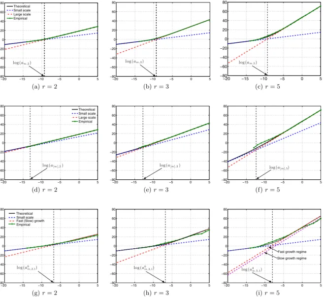
−20 −15 −10 −5 0 5 −80 −60 −40 −20 0 20 40 60 80 Theoretical Small scale Large scale Empirical
log (am ,2)
(a)r= 2
−20 −15 −10 −5 0 5 −80 −60 −40 −20 0 20 40 60 80
log (am ,3)
(b)r= 3
−20 −15 −10 −5 0 5
−80 −60 −40 −20 0 20 40 60 80
log (am ,5)
(c)r= 5
−20 −15 −10 −5 0 5 −80 −60 −40 −20 0 20 40 60 80 Theoretical Small scale Large scale Empirical
log (a[m],2)
(d)r= 2
−20 −15 −10 −5 0 5 −80 −60 −40 −20 0 20 40 60 80
log (a[m],3)
(e)r= 3
−20 −15 −10 −5 0 5 −80 −60 −40 −20 0 20 40 60 80
log (a[m],5)
(f)r= 5
−20 −15 −10 −5 0 5 −80 −60 −40 −20 0 20 40 60 80
log (a0 m ,2,1) Theoretical Small scale Empirical Fast (Slow) growth
(g)r= 2
−20 −15 −10 −5 0 5 −80 −60 −40 −20 0 20 40 60 80
log (a0 m ,3,1)
(h)r= 3
−20 −15 −10 −5 0 5 −80 −60 −40 −20 0 20 40 60 80
Fast growth regime Slow growth regime
log (a0 m ,5,1)
(i)r= 5
Figure 1. Top: moments (log-log scale); Middle: factorial moments (log-log scale); Bottom:
central moments (log-log scale).
them to be separated by a “knee,” the transition scale (or the range of such) where the behavior changes as one moves from one scaling behavior to another. The biscaling and the “knee” are clearly seen in Figure 1(to be discussed in more detail in Sect.7) where the factorial moments, moments and central moments are plotted on the log scale for both axes.
The location of the “knee” (i.e., the transition scale a) can be approximated by equating the scaling rela-tions for different scaling behaviors and quantities of interest, and solving with respect toa. For the factorial cumulants, by equating the relations (3.2) and (4.3), we obtain
ET AL.
and solving foraleads to the approximate location of the “knee” (the transition scale from small to large scales) given byaκ,[r]= (cκ,[r]/Cκ,[r])1/(r−(r−1)θ−α)or
aκ,[r]=
(r−2)!CF,r−1(EA)r−α(α−1)(r−α)(r+ 1−α)Rr
((r−1)θ+ 1)CW
1/(r−(r−1)θ−α)
, r≥2, (6.1)
by using the forms of the coefficients Cκ,[r] andcκ,[r]. Similarly, from Corollaries3.3 and4.3, the locations of
the “knee” (the transition scales) in the transition from small to large scales for the factorial moments and the usual moments are approximated by, respectively,
am,[r]=
r!CF,r−1Rr
λr−1((r−1)θ+ 1)(EW)r
1/(r−(r−1)θ−1)
, θ∈(0,1), (6.2)
am,r=
1
λEW, r≥2. (6.3)
We note that the location of the “knee” for the moments does not dependent on the orderrand the distribution of the interarrival times A. Whenθ >1, the factorial moments have the same asymptotics for both large and small scales. Whenθ= 1, the asymptotics are the same inabut differ in the multiplicative constants, and our approach does not yield a transition scale.
The case of the central moments is more delicate due to the effect of the slow and fast growth regimes discussed in Section 5. We note first that for fixed λand as a increases, the fast growth regime comes before the slow growth regime; indeed, asa→ ∞,λ/aα−1 →0 for fixed λ. Thus, for the central moments, we shall distinguish between two transition scalesa0m,r,1anda0m,r,2:a0m,r,1being the transition scale (“knee”) from small
scales into the fast growth, and a0m,r,2 being the transition scale (“knee”) from the fast growth into the slow growth. By equating (4.11) and (5.14) (in the fast regime) and solving foraleads to
a0m,r,1=
⎧ ⎪ ⎪ ⎪ ⎪ ⎪ ⎪ ⎪ ⎨ ⎪ ⎪ ⎪ ⎪ ⎪ ⎪ ⎪ ⎩ ⎛
⎝ r!Cr/
2
κ,[2]
EW(r/2)!2r/2λ r/2−1
⎞ ⎠
−2/((3−α)r−2)
, evenr≥2,
⎛
⎝ r!C
(r−1)/2−1 κ,[2] Cκ,[3]
EW((r−1)/2−1)!2(r−1)/2−13!λ
(r−1)/2−1
⎞ ⎠
−2/((r−1)(3−α))
, oddr≥2.
(6.4)
Similarly, equating (5.14) in the fast and slow regimes leads to
a0m,r,2=
⎧ ⎪ ⎪ ⎪ ⎪ ⎪ ⎪ ⎪ ⎨ ⎪ ⎪ ⎪ ⎪ ⎪ ⎪ ⎪ ⎩ ⎛
⎝ r!Cr/
2
κ,[2]
Cκ,[r](r/2)!2r/2
λr/2−1
⎞ ⎠
2/((r−2)(α−1))
, evenr≥4,
⎛
⎝ r!C
(r−1)/2−1 κ,[2] Cκ,[3]
Cκ,[r]((r−1)/2−1)!2(r−1)/2−13!
λ(r−1)/2−1
⎞ ⎠
2/((r−3)(α−1))
, oddr≥4.
(6.5)
(Recall from Sect.5 that there is difference in the two regimes only whenr≥4). As will be seen in Section7, the transition scalea0m,r,2may be too large to observe in practice.
For the usual cumulants, the location of the transition scale aκ,r, r≥ 2, from small to large scales follows
from (3.16) and (4.14), to yield
aκ,r =
(α−1)(r−α)(r+ 1−α)EW(EA)r−α
r(r−1)CW
1/(r−α)
, r≥2. (6.6)