Rational maps lacking certain periodic orbits

(1)

Rational Maps Lacking Certain Periodic Orbits

Rika Hagihara

A dissertation submitted to the faculty of the University of North Carolina at Chapel Hill in partial fulfillment of the requirements for the degree of Doctor of Philosophy in the Department of Mathematics.

Chapel Hill 2007

Approved by

(2)

ABSTRACT

RIKA HAGIHARA: Rational Maps Lacking Certain Periodic Orbits

(Under the direction of Professor Jane Hawkins)

This thesis is a study of the dynamics of rational maps without certain periodic points, focusing on the roles of critical points. We examine how the dynamics occurring within the parameterized family of exceptional rational maps are reflected in the parameter space.

We use Baker’s results on the multiplicities of fixed points of a rational map to give a complete proof of the classification of exceptional rational maps. In degree 2 and 3 cases exceptional rational maps form parameterized families, all of whose members have parabolic fixed point(s).

(3)

ACKNOWLEDGMENTS

My thesis advisor, Dr. Jane Hawkins, guided me to the beauty and complexity of complex dynamics. The amount of time and patience she had for me is beyond description. Without her encouragement this thesis simply would not exist. I thank her for her undeniable support over the past four years.

Also, thanks to Dr. Joseph Cima, Dr. Sue Goodman, Dr. Karl Petersen, Dr. Michael Taylor, and Dr. Warren Wogen for serving on my thesis committee. In particular, I am grateful to Dr. Michael Taylor for his comments on the earlier versions of the thesis.

My family, from one continent and one ocean away, did everything so that I could focus on my studies in the States. I thank them for their understanding and support.

(4)

LIST OF FIGURES

Figure 1.1. Π and Πr with r = 1,6. . . 9

Figure 1.2. Two petals. . . 11

Figure 1.3. One petal. . . 11

Figure 1.4. F(R[5;3;1;1],4i). . . 11

Figure 1.5. Siegel disk. . . 11

Figure 1.6. The parameter space of _{R(2,2),a}. . . 16

Figure 3.1. _R(2,2),a is the region inside the circle. . . 31

Figure 3.2. J(R(2,2),a) and J(g_◦R(2,2),f(a)◦g−1). . . 32

Figure 3.3. J(R(2,2),ω) and J(R(2,2),¯ω). . . 33

Figure 3.4. A blow-up. . . 33

Figure 3.5. c2 only. . . 33

Figure 3.6. A1, A2,A3, and A4. . . 35

Figure 3.7. Misiurewicz and center points. . . 53

Figure 3.8. The parameter space of _{Pc}. . . 55

Figure 3.9. M00_{. . . 58}

Figure 4.1. Ra,ω is the region inside the circle. . . 61

Figure 4.2. J(R[7;1;1:ω]) and J(R[4;4;1:ω]). . . 61

Figure 5.1. The parameter space pictures of (d, b) = (3,2) families . . . 67

Figure 5.2. Three curves for [3;3;3;1]. . . 72

Figure 5.3. _{R[3;3;3;1],a. . . 75}

Figure 5.4. Blow up of the parameter space for {R[3;3;3;1],a}. . . 79

Figure 5.5. Period 3 Mandelbrot set and the dynamical plane. . . 80

Figure 5.6. Three curves for [7;1;1;1]. . . 83

(7)

Figure 5.8. _{R[7;1;1;1],a}sketched by a unique critical point. . . 85

Figure 6.1. J(R[13;1;1;1;1]). . . 88

Figure 6.2. J(R[9;5;1;1;1]). . . 88

Figure 6.3. J(R[7;3;3;3;1]). . . 89

(8)

CHAPTER 1

Preliminary Definitions and Notation

1.1. Overview

In the theory of the iteration of rational maps, the question one should ask is, “What are the roles of the critical points?” This dissertation gives partial answers in the case of the family of rational maps lacking certain periodic orbits, focusing on the behavior of the critical points under iteration.

In Chapter 1, we summarize standard definitions, notation, and results of complex dynamics that are used throughout this thesis.

In Chapter 2, we give a complete proof of the classification of rational maps lacking certain periodic orbits. Periodic points play an important role in the theory of iteration of rational maps. Every rational map has infinitely many periodic points [2]. However, there are rational maps R without periodic points of a certain period. Baker [1] proved that if a polynomialP has no periodic points of periodn, thenn = 2 andP is conjugate to z 7→ z2 ₋_z_{. As for rational maps of degree} _d _{without period} _n _{orbits, he obtained} the list of the pairs (d, n). Although Kisaka [9] exhausted all tweleve possible forms of such maps, his three-and-a-half-page paper contained no proofs except two cases. So the proofs of Corollaries 2.8-2.10 as well as the exposition of the classification are original.

The detailed dynamical study on rational maps without certain periodic orbits begins in Chapter 3. Here we study the family of rational maps R(2,2),a(z) = z

2₋_z

(9)

no period 2 orbits. First we obtain the reduced region for _{R(2,2),a} from its parameter space using conformal conjugacy. We also show that symmetry reduces the study of the reduced region. Next we show that for parameters on certain components in the reduced region the dynamics of the corresponding maps can be thoroughly understood. Further, we prove that in some cases the dynamics can be explained with marked critical points. The main result of Chapter 3 is the following theorem.

Theorem 3.11 The orbit of the critical point c1 = −1+

√

1+a

a of R(2,2),a converges to the parabolic fixed point 0 for each parameter value a in the following sets.

A1 ={a∈ R(2,2),a : |a|<1};

A2 ={a∈ R(2,2),a : −3≤a <−1};

A3 ={a∈ R(2,2),a : Re

a+ 4

a+ 1

<−3};

A4 ={a∈ R(2,2),a : |a+ 1|= 2,

π

2 <Arg(a+ 1)< π}.

For parameter values in A1, the orbit of the critical point c2 converges to the attracting fixed point_∞. For parameter values inA2,A3, andA4, the iterates of both critical points

c1,c2 converge to 0. For parameter values in A4 the iterates of both critical points lie on the circle with center 2

1−a (another fixed point ofR(2,2),a) and radius

2

1−a

.

Finally, we compare similarities and dissimilarities between _{R(2,2),a} and the pa-rameterized family of quadratic polynomials, both on the parameter space level and the dynamical plane level.

(10)

is always the same for b _∈ S1_{\ {}₁_}_{. This is Corollary 4.3. We also give more details of} some examples found in Milnor [13].

In Chapter 5 we study the degree 3 rational maps without period 2 orbits. Our main goal is to obtain the reduced region of each family of degree 3 exceptional maps and describe the dynamics occurring within the family. We list the maps generating the equivalence classes and give a description of the reduced regions. The mains results in this chapter are Corollary 5.4 and Theorems 5.5 and 5.6. In some cases, interesting dynamics are shown with computer generated pictures.

In Chapter 6, we explain why the dynamics of the degree 4 rational maps lacking period 2 orbits are well-understood.

Lastly, we discuss other questions that are relevant to this thesis and that we hope to investigate further in the future.

Neutral fixed and periodic points are rarely studied, and in fact, except for some expository examples in [13] the author is not aware of any study of parameterized fam-ilies of rational maps all of whose members have parabolic fixed point(s), making both mathematics and computer visualization difficult.

Some computer programs are edited versions of Mathematica programs first written by Lorelei Koss. Others were written in C++ by Paul Rowan using algorithms by P. Rowan and J. Hawkins.

1.2. Preliminary Definitions and Notation

(11)

The orbit of a point α∈Cb _{under iteration by} _R _{is the sequence}

α, R(α), R2(α), _{· · ·} , Rn₍_α₎_, · · · .

A point α is a periodic point of R of period n if Rn₍_α_{) =}_α_{, where} _Rn _{denotes the} _n_-th iterate of R and n is the smallest positive integer satisfying this relation. If n = 1, α is called a fixed point.

If a rational function R is written as R(z) = P(z)/Q(z) using coprime polynomials

P and Q, then the degree of R is defined by degR = max{degP,degQ}.

If R is a rational map and S =ϕ◦R◦ϕ−1 _{for some} _ϕ_∈ _Aut(_Cb_{), then} _S _{is said to} be (conformally) conjugate to R. Conjugacy is an equivalence relation, and we do not distinguish rational maps in the same equivalence class (conjugacy class). Conjugation respects fixed points.

1.3. Fatou and Julia Sets

The Fatou set F(R) of R is the maximal open subset of Cb _{in which} _{_Rn_}n

∈N forms

a normal family. The Julia set J(R) is the complement of the Fatou set. The Fatou set F and the Julia set J are completely invariant under R: R−1₍_F_{) =}_F ₌ _R₍_F_{) and}

R−1₍_J_{) =}_J ₌_R₍_J_{). Also, for any positive integer}_n_,_F₍_Rn_{) =}_F₍_R_{) and}_J₍_Rn_{) =} _J₍_R_). If degR≥2, then J(R) is a perfect set, and either J =Cb _or_J _{has empty interior [}₂_].

1.4. Classification of Periodic Points

In order to state how the periodic points relate to the Fatou and Julia sets, we need to classify periodic points. The multiplierof a fixed point α _∈C _{of a rational map} _R _is

(12)

m(R,_∞) = limz_→01/R0₍₁_/z_{). Next, we extend this notion to periodic points. Suppose}

that α is a periodic point of R with period n, and write αi = Ri(α), 0 ≤ i ≤ n−1. Then _{α0,· · · , αn−1}is the cycleof α. By conjugation we may assume that ∞ is not in the cycle. Then (Rn₎₀₍_α_{i) is independent of the choice of a point} _α

i in the cycle. This number is the multiplier of the cycle, and is denoted by m(Rn_{, α}_{i). Depending on the} value of the multiplier, a periodic point αi or its cycle is called

(i) super-attractingif m(Rn_{, α}_{i) = 0;} (ii) attracting if 0<_|m(Rn_{, α}_i)

|<1; (iii) neutral if _|m(Rn_{, α}_i)

|= 1; (iv) repelling if |m(Rn_{, α}_i)_|_>_1.

A neutral periodic pointαior its cycle isparabolicifm(Rn, αi) is a root of unity; otherwise it is called irrational. Note that conjugation preserves multipliers.

1.5. Dynamics near Periodic Points

The following theorems summarize some relations between periodic points and the Fatou and the Julia set. Throughout, we suppose thatRis a rational map with degR ≥2.

1.5.1. (Super-)Attracting Periodic Points. For simplicity assume thatRhas a fixed point 0 with m(R,0) =λ, and the Taylor series of R at 0 is written as

R(z) =λz+bzr+1+ O(zr+2)

where b is the first non-zero coefficient with r≥1.

(13)

and using Vitali’s Theorem we can gain information on the limit of the sequence _{Rn_} on a component of F(R) containing D.

Theorem 1.1. ([2]) (Vitali’s Theorem) Suppose that the family {fn}n_∈N of analytic

maps is normal in a domain X, and that fn converges pointwise to some function f on

some non-empty open subset Y of X. Then f extends to a function F which is analytic

on X, and fn →F locally uniformly on Y.

Vitali’s Theorem implies that Rn _→ _{0 locally uniformly on the component of} _F₍_R₎ containing D. In general, we have the following Theorem.

Theorem1.2. ([2])If _{α0, α1,· · · , αn−1}is a (super-)attracting cycle ofR, then each

αi lies in some Fatou component Fi and as m → ∞, (Rn)m → αi locally uniformly on

Fi.

1.5.2. Parabolic Periodic Points. The parabolic case is significantly different from the (super-)attracting case since R is not conjugate to its linear derivative map in an open neighborhood of a parabolic fixed point. To see this, suppose thatRhas a parabolic fixed point 0 with m(R,0) = λ, and R is conjugate to λz near 0 and λn _{= 1 for some}

n _∈ N_{. Then} _Rn _{is conjugate to the identity map. The conjugacy class of the identity}

map consists of only the identity map, hence Rn _{= id, which is a contradiction since} degR ≥2 by assumption.

Instead, we consider a conjugacy on some open set that has 0 on its boundary. We first cite a theorem, and then consider the parabolic case in several steps.

(14)

Case 1. λ = 1, r = 1. Then R is conjugate to a map (denoted again by R) whose Taylor series at 0 is

R(z) =z−z2+ O(z3).

Conjugating R with f(z) = 1

z amounts to the change of coordinates:

(f ◦R◦f−1)(z) =z+ 1 + c

z +· · · .

Then_∞has a neighborhood Π =_{x+iy: y2 _>₄_K₍_K₋_x₎_}_{bounded by a parabola with} someK >0, and the following can be shown: (f_◦R_◦f−1_)(Π)_⊂_{Π; (}_f_◦_Rn_◦_f−1₎₍_z₎_{→ ∞} uniformly on Π; f _◦R_◦f−1 _{: Π}_→_{Π is conjugate to a translation} _z_7→_z_{+ 1.}

Setting Π0 = f−1_{(Π), we see that} _R_(Π0) _⊂ _Π0, _Rn _→ _{0 uniformly on Π0, and}

R : Π0 →Π0 is conjugate to a translation. From these we deduce that Π0 ⊂ F(R), and an application of Vitali’s Theorem implies that Rn _→ _{0 locally uniformly on a Fatou} component F0 containing Π0. Since parabolic periodic points are in J(R), the parabolic fixed point 0 is on the boundary of Π0 as well as F0.

Also, the region Π0 can be seen to have a cardioid shape: it is symmetric about the real line and makes an angle 2π at 0 (so 0 is a cusp point). See Figure 1.1. Moreover, it can be proven that the iterates of a point inF0 approach 0 in a direction tangent to the positive real axis.

Case 2.λ = 1, r >1. ThenR is conjugate to a function (denoted again by R) whose Taylor series at 0 is

(1) z0 =R(z) =z−zr+1+ O(z2r+1).

Change variables by z = ζ1r and z0 = ζ0

1

r, where ζ and ζ0 are in the same sheet of the

(15)

z and z0 _{are in a sector with aperture} 2π

r . Then (1) becomes

ζ0 =ζ₋rζ2+ O(_|ζ_|2+1r).

Renormalize r, and change coordinates by z = 1

ζ and z0 = 1

ζ0 to obtain

z0 =z+ 1 + O(_|z_|−1r).

We then proceed as in Case 1 to show that there are r “petal”-shaped regions Πi, i = 0, . . . , r ₋1, each making an angle 2π

r at 0. They satisfy R(Πi) ⊂ Πi, and R n

→ 0 uniformly and asymptotically to the ray _{z : Arg(z) = 2πi_r _} on Πi. Hence each Πi is in

F(R), say Πi ⊂Fi for some Fatou componentFi, andRn(z)→0 locally uniformly while Arg (Rn₍_z₎₎_→ 2πi

r on each Fi. From the last statement we see thatFi∩Fj =∅fori6=j. We summarize Cases 1 and 2 in the next Theorem.

Theorem 1.4. ([2]) Let 0 be a parabolic fixed point of R with m(R,0) = 1. Then

0∈J(R). If R has the Taylor series

R(z) =z+bzr+1+ O(zr+2)

at 0where b is the first non-zero coefficient with r≥ 1, then there are r petalsΠi each of angle 2π_r at 0. There exist disjoint components {Fi}_i=0r−1 of F(R), each containing a petal

based at 0, Πi _⊂Fi. Moreover, R maps each Fi onto itself, and as n → ∞, Rn(z) →0

locally uniformly on Fi.

In Figure 1.1 the shaded region bounded by a parabola y2 _{= 4}_K₍_K₋_x_{) (left) is Π.} It is mapped by z _7→ z−1

(16)

-10 -5 0 5 10 -10

-5 0 5 10

-0.4 -0.2 0 0.2 0.4

-1 -0.5 0 0.5 1

Figure 1.1. Π and Πr with r= 1,6.

Case 3. λ₆= 1 but λn _{= 1. Theorem 1.4 can be extended to a parabolic fixed point 0} whose multiplier is other than 1. Suppose that m(R,0) is a primitive n-th root of unity. Then 0_∈J(R), and it can be shown [1] that the multiplicity of 0 as a fixed point ofRn_is of the formnk+ 1 for some positive integerk. So, there arenkpetals, each of angle 2π_nk at 0. There exist nkdisjoint components of F(R), each containing a petal. R acts on them as a permutation on k disjoint cycles each of length n, and as m → ∞, (Rn₎m₍_z₎ _→ ₀ on each such component of F(R). The extension of Theorem 1.4 to a parabolic cycle is similar. This completes the description of dynamics near a parabolic fixed and periodic point.

(17)

Case 3 there are k disjoint immediate basins of a parabolic fixed point each of length n. Also, see Example 1.7.

Example 1.5. The Fatou set of R(2,2),0(z) = z2 ₋_z_{. The rational map} _R

(2,2),0 has an attracting fixed point ∞, a parabolic fixed point 0 with m(R(2,2),0,0) = −1, and a repelling fixed point 2. The immediate basin of_∞is completely invariant. The immediate basin of 0 consists of two cyclic components of F(R(2,2),0). Each of these components contains a conformal image of a petal making an angle of π at 0. See Figure 1.2. The range is_{−1,2_{} × {−}1.5i,1.5i_}.

Example 1.6. The Fatou set ofR(2,2),1(z) = z

2₋_z

z+1. The rational map R(2,2),1 has two parabolic fixed points 0 and ∞. The immediate basin of ∞ is a completely invariant Fatou component. It contains a conformal image of a cardioid-shape petal making an angle of 2π at _∞. In Figure 1.3, R(2,2),1 is conjugated by f(z) = 1z to switch ∞ and 0. The range is_{−2.5,1.5_{} × {−}2i,2i_}.

Example 1.7. The Fatou set ofR[5;3;1;1],4i(z) = z3−z

−z2_+4iz+1. Two of the fixed points α1 andα2coincide at the parabolic fixed pointiofRwith multiplicity 2. All the gray regions are eventually mapped onto the immediate basin of the fixed pointi(as a consequence of No Wandering Domains Theorem in Section 1.6). Also, the map R has a parabolic fixed point 0 with multiplicity 5. There are two disjoint immediate basins of R at 0. Each of these consists of two cyclic Fatou components, and they are placed diagonally at 0. The immediate basin of another parabolic fixed point_∞consists of two cyclic components of

(18)

-1 -0.5 0 0.5 1 1.5 2 -1.5

-1 -0.5 0 0.5 1 1.5

Figure 1.2. Two petals.

-2 -1 0 1

-2 -1 0 1 2

Figure 1.3. One petal.

-4 -2 0 2 4

-6 -4 -2 0 2 4

Figure 1.4. F(R[5;3;1;1],4i).

-2 -1 0 1 2

Figure 1.5. Siegel disk.

(19)

Theorem 1.8. ([2]) An irrational fixed point 0 of R is in the Fatou set if and only if R is analytically conjugate to its linear derivative map R0₍₀₎_z _near ₀_{. Moreover, the} Fatou component containing 0is simply connected and in it R is (analytically) conjugate to an irrational rotation of the unit disk.

Such a Fatou component is called a Siegeldisk.

Theorem1.9. ([2])For Lebesgue almost every θ_∈R_/Z_{any analytic function} _f _with the Taylor series f(z) =e2πiθ_z_{+ O(}_z2₎ _{is linearizable near} ₀_.

If an irrational fixed point α of R is in J(R), then α is called a Cremer point.

Example 1.10. The Siegel disk at_∞ ofR(2,2),e2πiθ(z) = z

2₋_z

e2πiθ_z₋₁ whereθ = 1+

√

5 2 (the golden mean). The fixed point_∞of R(2,2),e2πiθ with multipliere2πiθ is in a Siegel disk (see [7], p.84). In Figure 1.5, R(2,2),e2πiθ is conjugated by f(z) = 1

z so that ∞ is interchanged with 0. The range of Figure 1.5 is {−2,2} × {−2i,2i}.

1.5.4. Repelling Periodic Points. As for the repelling periodic points, we have the following Theorem.

Theorem 1.11. ([2]) The set of repelling periodic points is dense in J(R).

If 0 is a repelling fixed point of R with m(R,0) = λ, then there is a branch of R−1 for which 0 is an attracting fixed point with multiplier _λ1 ([2], [7]). Any map locally conjugating R−1 _to z

λ (linear derivative map) also conjugates R to λz near 0.

1.6. Classification of Fatou Components

(20)

Theorem 1.12. ([2], [11]) (No Wandering Domains Theorem) Every component of the Fatou set of R is pre-periodic, i.e., for every component U of F(R), there exist integers 0_≤l < m with Rl₍_U_{) =}_Rm₍_U₎_.

The No Wandering Domains Theorem together with the theorem below completely classifies the components ofF(R).

Theorem1.13. ([11])IfV is a periodic component ofF(R)andr∈N_{is the smallest} positive integer such that Rr₍_V_{) =}_V_{, then} _V _{is one of the types} _(i)_-_(iv)_:

(i) an attracting component: V contains a (super-)attracting periodic point α and as n _{→ ∞}, (Rr₎n₍_z₎_→_α _{locally uniformly on} _V_;

(ii) a parabolic component:there is a parabolic periodic point α of R on the bound-ary of V, and as n→ ∞, (Rr₎n

(z)→α locally uniformly;

(iii) a Siegel disk: Rr _:_V _→_V _{is analytically conjugate to an irrational rotation of}

the unit disk onto itself;

(iv) a Herman ring: Rr _: _V _→_V _{is analytically conjugate to an irrational rotation}

of some annulus onto itself.

1.7. Critical Points

To study the dynamics of a rational map R thoroughly, we must analyze the role of critical points. A point z is a critical point of R if R0₍_z_{) = 0. If deg}_R ₌ _d_{, then} _R _has

at most 2d−2 critical points in Cb_{: moreover, a quadratic map always has two distinct}

(21)

Theorem 1.14. ([2])Let C+₍_R₎_{be the set of the forward images of critical points of}

R.

(i) Each immediate basin of a (super-)attracting or parabolic cycle of R contains a critical point of R;

(ii) The union of the boundary of a cycle of Siegel disks or Herman rings is contained in the closure of C+₍_R₎_;

(iii) Each irrationally neutral cycle of R in J(R) lies in the derived set of C+₍_R₎_.

1.8. Critical Points and Parameter Space

Generally speaking, the dynamics of a parameterized family of rational maps{Ra}a_∈C,

such as the types of fixed or periodic points, change as the parameter value changes. In turn the changes in the dynamics are often reflected on the behavior of the forward iterates of the critical points. To investigate the behavior of the critical points of Ra and hence the dynamics ofRa further, we define the parameter spaceas the a-plane, and produce the parameter space picture of_{Ra}. The algorithm basically tracks the forward iterates of the critical points ci.

Computer Algorithm for Producing the Parameter Space of _{Ra}.

(i) Each pixel represents a parameter valueacorresponding to the mapRa. Assign the default value 0 to each a.

(ii) For eacha, we iterate the critical pointsN >0 times to start. Letsi =RaN(ci). (iii) Choose > 0 and set M ∈ N _{to be the maximal number of iterations. Apply}

the following test for each ci: If the inequality |Ran(si)−si|< is satisfied in either the Euclidean or spherical metric for some n _∈ N_{, where 0} _≤ _n _≤ _M_,

(22)

(iv) Assign to each a the number of times the value 1 is assigned in (iii). Shade the parameters a according to these numbers so that the parameters with the biggest number are colored white, and the parameters with the smallest number are colored black.

The algorithm is supported by the following reasons. Generally speaking, if an at-tracting cycle has a small multiplier, then the iterates of the associated critical point(s) in the attracting immediate basin approach the points in the cycle quite quickly. This enables the inequality in (iii) to hold. Also, if a critical point is associated with a para-bolic cycle, then although the attraction is very, very slow so we many have to take many iterations (by letting N and n be large), the inequality in (iii) eventually holds. On the other hand, if a critical point is associated with a cycle of Siegel disks or Herman rings, then the image of the critical point after a finite number of iterations may not return near the critical point itself. This results in the inequality in (iii) being false for most

>0 and mostn.

For a fixed parametera when we discuss and show the Julia and Fatou sets for Ra in

b

C_{, we refer to it as the} _{dynamical plane}_for_R_a_{in order to contrast it with the parameter}

plane.

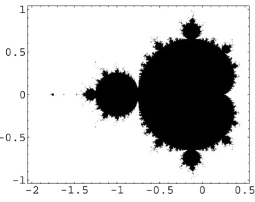
Example 1.15. The parameter space picture of {R(2,2),a}. The parameter space picture of{R(2,2),a}, whereR(2,2),a(z) = z

2₋_z

az+1, is given in Figure 1.6. The range is{−2,2}× {−6.5i,6.5i}. Each R(2,2),a has two critical points c1 = −1+

√

1+a

a and c2 =

(23)

-2 -1

0

1

2 -6

-4

-2

0

2

4

6

(24)

CHAPTER 2

Possible Combinations of Multiplicities

2.1. Baker’s Proposition

Ifd_≥1, a rational mapRof degreedhasd+1 fixed points inCb _{counting multiplicity.}

Every rational mapR has infinitely many periodic points (Beardon [2]). However, as the following example shows, there are rational maps without periodic points of a certain period.

Example 2.1. R(2,2),0(z) =z2−z. The three fixed points of R(2,2),0 inCb are 0,2, and ∞. The five fixed points of R(2,2),02 in Cb are 0,0,0,2, and ∞. So R(2,2),0 does not have period 2 points.

Question 2.2. ([1], [2]) To quote Beardon, “How often are periodic points absent?”

The following are due to Baker [1]:

Theorem 2.3. ([1]) If a polynomial P of degree at least 2 has no periodic points of period n, then n = 2 and P is conjugate to z _7→z2₋_z_.

(25)

A rational map R on Cb _{is said to be} _exceptional _{if it lacks periodic points of a}

certain period. Although Baker gives an example of a rational map to illustrate each of the four exceptional cases, his example corresponding to the case (d, n) = (4,2) is incorrect (Kisaka [9]). Also, as Beardon points out, “[N]ot only is Theorem 2.4 weaker than Theorem 2.3 in that several exceptional pairs (d, n) arise, but it is also weaker in that an exceptional pair (d, n) does not necessarily determine a unique conjugacy class of exceptional maps R.”

Question 2.5. Can rational maps be specified for each exceptional case up to con-jugacy?

Kisaka [9] exhausted all possible forms of exceptional rational maps up to conjugacy. It turns out that many of the exceptional rational maps contain parameters. In general, dynamics occurring within a parameterized family of rational maps depend on the pa-rameter values. However, Kisaka failed to mention this, nor did he develop the subject beyond the three and a half pages listing the cases.

As mentioned in Milnor [13] (for (d, n) = (2,2)) and [9] (for (d, n) = (2,2) and (2,3)), if a degreedrational mapR has no period n points and if the pair (d, n) is either (2,2),(2,3),(3,2) or (4,2), then each periodn cycle is supposed to degenerate to a fixed point. Corollary 2.8 algebraically produces the list of the resulting multiplicities of the fixed points of Rn_{. This enables us to state the procedure, applicable to all exceptional} cases, to classify exceptional rational maps.

(26)

Proposition 2.6. ([1]) If f and fn _{are analytic at} _α_, _n _∈ _Z

+ , and z = α is a

solution both of

f(z)−z = 0 (1)

and fn₍_z₎

−z = 0,

(2)

then

(i) α is a simple root of both equations unless (f0₍_α₎₎n_{= 1}_;

(ii) if f0₍_α_{) = 1} _then _α _{has the same multiplicity} ₍_>₁₎ _{for both equations;}

(iii) if α is a multiple root of (3) and f0₍_α₎ _{is a primitive} _t_{-th root of unity with} t > 1, then the multiplicity of α in (2) is 1, while in (3) it is an integer of the form tk+ 1, where k is a positive integer. Moreover, t|n .

Proof. If we write the Taylor series off at α as

f(z) =α+a(z₋α) +_{· · ·} ,

then the Taylor series of fn _at _α _{is given by}

fn(z) =α+an(z−α) +· · · .

With these, equations (2) and (3) can be written as

(z₋α)_{· {}(a₋1) + O(z₋α)_}= 0

and

(z₋α)_{· {}(an

−1) + O(z₋α)_}= 0,

respectively. If an_{= (}_f0₍_α₎₎n

6

(27)

For (ii), note that if

f(z) =α+ (z₋α) +b(z₋α)r+1+_{· · ·}

where b is the first non-zero coefficient with r≥1, then

fn₍_z_{) =}_α_{+ (}_z

−α) +nb(z₋α)r+1+_{· · ·} .

With these, equations (2) and (3) are written as

b(z₋α)r+1_{1 + O(z₋α)_}= 0

and

nb(z−α)r+1{1 + O(z−α)}= 0,

respectively. Hence both equations have r+ 1 solutions at α counting multiplicity. To prove (iii), first note that ifα is a multiple root of (3), then an_{= (}_f0₍_α₎₎n

= 1 by (i), so that t_|n. Furthermore, if

fn(z) =α+ (z−α) +c(z−α)s+1+· · ·

wherecis the first non-zero coefficient withs ≥1, then by substituting the Taylor series forf andfn_{into the identity} _f₍_fn₍_z_{)) =}_fn₍_f₍_z_{)) and identifying coefficients, we obtain}

as _{= 1, so that} _t_|_s_{. Thus, the multiplicity} _s_{+ 1 of} _α _{as a solution of (3) must be of the}

formtk + 1 with k_≥1.

From Proposition 2.6 we obtain the following Corollaries.

Corollary 2.7. ([2]) With the notation and statements from Proposition 2.6, the multiplicity of α as a solution of equation (3) is equal to or higher than that of (2). If it is higher, then (f0₍_α₎₎n

(28)

Corollary 2.8. Suppose that a rational map R has degree d with d _≥ 2, and α0, α1, . . . , αd are d+ 1 (not necessarily distinct) solutions of

(3) R(z)₋z = 0

in Cb_{. If}_n _{is prime, then the multiplicity of} _α_i_{, i}_{= 0}_,₁_{, . . . , d}_{, in}

(4) Rn₍_z₎

−z = 0

is an integer of the form nki + 1, where ki ∈ Z+. If αi = αj, then the multiplicity is (nki+ 1) + (nkj+ 1) with ki =kj = 0.

Proof. Note that if n is prime, then t = n in Proposition 2.6. By conjugation, we may assume that all fixed points of R are inC_.

(i) If (R0₍_α_i))n ₆_{= 1, then} _α

i is a simple root of both equations (so ki = 0) by Proposition 2.6 (i).

(ii) If R0₍_α_{i) = 1, then} _α

i coincides with other fixed point(s), and the fixed point has multiplicity r _≥2. In other words, there is a set A_{⊂ {}0, 1, _{· · ·} , d_}, where

i _∈ A and _|A_| = r, such that if j _∈ A, then αi = αj. Then the multiplicity of this point in both equations (4) and (5) can be expressed as P_j_∈_A(nkj + 1) with kj = 0 for allj ∈A.

(iii) If R0₍_α_{i) is a primitive} _n_{-th root of unity, and moreover if} _α

i is a simple root of (4) and a multiple root of (5), then Proposition 2.6(iii) implies that the multiplicity of αi as a solution of (5) is an integer of the form nki+ 1, where

ki ≥1.

(29)

From Corollaries 2.7 and 2.8 we obtain the following Corollary.

Corollary 2.9. If n is prime, then the following are equivalent.

(i) The multiplicity of α as a fixed point of Rn _{is strictly greater than that of} _R_; (ii) R0₍_α₎ _{is a primitive} _n_{-th root of unity;}

(iii) If k corresponds to α in Corollary 2.8, then k₆= 0.

Proof. Corollary 2.7 implies (i)_⇒(ii). The directions (ii)_⇒(iii) and (iii)_⇒(i) follow from

Corollary 2.8.

Corollary 2.10. ([9])If a rational mapR fails to have any periodic points of period n, then R cannot have one and only one fixed point.

Proof. Suppose that a rational function R of degree d has one and only one fixed point

α with multiplicity d+ 1. Then the equation R(z)₋z = 0 is of the form

(z₋α)d+1_·(non-zero coefficient) = 0.

So in the Taylor series of R(z)₋z atα,

(R0(α)₋1)_·(z₋α) +R00₂(α)_·(z₋α)2+_{· · ·}+R(d_d!)(α)_·(z₋α)d+R(_(d+1)!d+1)(α)_·(z₋α)d+1+_{· · ·} ,

coefficients of the terms of degree less thand+ 1 must be 0; in particular, the coefficient

R0₍_α₎₋_{1 of (}_z₋_α_{) is 0. By Proposition 2.6(ii) both}_R _and _Rn _have _α _{as a fixed point} with multiplicity d+ 1. However, Rn _has _dn_{+ 1 fixed points in} _Cb _{counting multiplicity,} and if (d, n) is one of the pairs (2,2), (2,3), (3,2), or (4,2), then (dn_{+ 1)}₋₍_d_{+ 1)} _>_0. Also, note that for (d, n) = (2,3), the map R3 _{does not fix periodic points of period 2.}

(30)

Corollary 2.10 implies that if a degreedrational map Rfails to have period n points, then R must have at least two distinct fixed points; without loss of generality choose 0 and _∞ as fixed points of R. Such a rational map can be written as

R(z) = bdz d₊_b

d−1zd−1+· · ·+b1z

ad₋1zd−1+· · ·+a1z+a0

,

wherebd 6= 0, a0 6= 0, and the numerator and the denominator have no common factors. By conjugation it can be assumed that 0 and∞ are the fixed points ofRn _{of the highest} and the second highest multiplicity, respectively. Dividing both numerator and denomi-nator bya0 and conjugatingR by an appropriate function of the form f(z) =λz so that the coefficient of zd _{becomes 1, we can assume}

R(z) = z d ₊_b

d₋1zd−1 +· · ·+b1z

ad−1zd−1 +· · ·+a1z+ 1

.

Applying Corollary 2.8 and re-labeling fixed points if necessary, without loss of generality the following must hold:

Xd

i=0(nki+ 1) =d n

+ 1 ; (5)

0_≤kd ≤kd−1 ≤ · · · ≤k0. (6)

SinceRn _{has more fixed points counting multiplicity than}_R _{has, at least one of the fixed} points ofR must have a higher multiplicity as a fixed point ofRn_{. Corollary 2.9 implies} that this happens when ki 6= 0. Then for the corresponding fixed point αi,

R0(αi) is a primitive n-th root of unity,

(31)

Now Baker’s Proposition 2.6 says that the multiplicity of αi as a fixed point ofRn is an integer of the form nki+ 1, and hence in the Taylor series of Rn at αi,

the coefficients of (z₋αi)m _{for all} _m _{with 2}

≤m_≤nk must be 0.

(8)

Note that ifα =∞, we need to consider the Taylor series of 1/Rn₍₁_/z_{) at 0.}

We now turn to an explicit classification of the rational maps R of degree d with no periodic points of period n. Our starting point is the list (d, n) of Theorem 2.4. With (5) and (6) the multiplicity of each fixed point of Rn _{can be specified; then (7) and (8)} determine the coefficients of polynomials in the denominator and the numerator of R.

2.2. Case 1. (d, n) = (2, 2)

From (5) and (6) we obtain [3; 1; 1] as the only possible combination of multiplicities of the fixed points (0; ∞; α) of R2_{. With} _R0_{(0) =} _b

1 = −1, the rational function takes the form

R(2,2),a(z) = z 2₋_z

az+ 1. Then ([2])

(i) R(2,2),a has fixed points 0, ∞, and α= ₁₋2_a;

(ii) the five fixed points ofR(2,2),a2 are 0, 0, 0, ∞, and α; (iii) R(2,2),a has no period 2 points.

Corollary 2.11. ([9], [13]) In order for a quadratic rational map to have no period 2 points, it is necessary and sufficient that one of its fixed points has multiplier −1.

(32)

conjugacy classes of the form z2₋_z

az+1 are not always unique. This family is studied in Chapter 3.

2.3. Case 2. (d, n) = (2, 3)

From (5) and (6) we obtain [7; 1; 1] and [4; 4; 1] as the possible combinations of mul-tiplicities of the fixed points (0; _∞; α) of R3_{. Since} _R0_{(0) =}_b

1 must be a primitive cube root of 1, the rational map has the form

R(z) = z 2 ₊_ωz

a1z+ 1

or R(z) = z

2₊_ω2_z

a1z+ 1

whereω =e2πi3 .

(i) For [7; 1; 1] we obtain

R[7;1;1:ω](z) =

z2₊_ωz

(−2−√3i)z+ 1 and R[7;1;1:ω2](z) =

z2₊_ω2_z (−2 +√3i)z+ 1.

(ii) For [4; 4; 1] we note that the multiplier ofR at_∞, limz_→∞1/R0₍₁_/z_{) =}_a_{1, must}

be a primitive cube root of unity. Also, the determinant of the matrix

   

1 ω

a1 1

   

forR(z) = z 2₊_ωz

a1z+ 1

       

1 ω2

a1 1

  

 forR(z) =

z2₊_ω2_z

a1z+ 1

,respectively

  

cannot be

1, for otherwise the numerator and the denominator ofRare not coprime. With these the rational function must be of the following:

R[4;4;1:ω](z) = z 2₊_ωz

ωz+ 1 and R[4;4;1:ω2](z) =

z2 ₊_ω2_z

ω2_z_{+ 1} .

(33)

2.4. Case 3. (d, n) = (3, 2)

From (5), (6), (7), and (8) we obtain the following as the possible combinations of multiplicities of the fixed points (0; _∞;α1; α2) of R2 and the associated rational maps

R:

[7; 1; 1; 1] :R[7;1;1;1],a(z) = z

3₊_az2₋_z

(a2₋₁₎_z2 ₋₂_az_{+ 1}, a∈C\ {0};

[5; 3; 1; 1] :R[5;3;1;1],a(z) = z 3₋_z

−z2 ₊_az_{+ 1}, a∈C\ {0}; [3; 3; 3; 1] :R[3;3;3;1],a(z) = z

3₋₂_az2₋_z −z2₋ 2

az+ 1

, a_∈C_{\ {}₀_,_±_i_}_.

2.5. Case 4. (d, n) = (4, 2)

From (5) and (6) we obtain the following as the possible combinations of multiplicities of the fixed points (0; ∞; α1; α2; α3) of R2_:

(i) [13; 1; 1; 1; 1], (ii) [11; 3; 1; 1; 1], (iii) [9; 5; 1; 1; 1], (iv) [9; 3; 3; 1; 1],

(v) [7; 7; 1; 1; 1], (vi) [7; 5; 3; 1; 1], (vii) [7; 3; 3; 3; 1], (viii) [5; 5; 5; 1; 1],

(ix) [5; 5; 3; 3; 1], (x) [5; 3; 3; 3; 3].

To show that case (x) does not happen, we use the following Lemma:

Lemma 2.13. ([14]) If the multiplier λi of a fixed point αi of a rational map R is not 1 for all i, then

X

i 1 1−λi

= 1.

(34)

(8) we see that cases (ii), (iv), (v), (vi), and (ix) cannot occur.

(i) R[13;1;1;1;1](z) = z 4 ₋_z −2z3_{+ 1}; (iii) R[9;5;1;1;1](z) =

z4₊_z3 ₊_z2₋_z −z3₊_z2₋₃_z_{+ 1};

(vii) R[7;3;3;3;1](z) = z 4 ₋₃1

3z3+ 323z2−z

−z3_{+ 3}4₃_z2 ₋₅_·₃−1 3 z+ 1

;

(viii) R[5;5;5;1;1](z) = z

4₊ −5+√5 2 z3+

3−√5 2 z2−z −z3₊ 3+√5

2 z2 +− 5−√5

2 z+ 1

.

2.6. Conclusion

(35)

CHAPTER 3

Degree two rational maps with no period two orbits:

(

d, n

) = (2

,

2)

3.1. A Parameter Space Study

To investigate all possible dynamics of quadratic rational maps with no period 2 cycles, we need only study the family of maps R(2,2),a(z) = z

2₋_z

az+1, a ∈ C\ {−1}. This section is organized as follows. We first obtain preliminary results on the fixed points of

R(2,2),a. This illustrates the dependence of the dynamics occurring within{R(2,2),a}on the parameter values a. Second, we reduce the parameter space using conformal conjugacy among_{R(2,2),a}. For distinct parameter values aand a0, the maps R(2,2),a and R(2,2),a0 in

the same parameterized family may be conformally conjugate, so in the dynamical point of view a and a0 _{play the same role in the parameter space. We define the equivalence}

relation ∼ on the parameter space by a ∼ a0 _{if and only if the corresponding maps} R(2,2),a and R(2,2),a0 are conformally conjugate. Then we form areduced region R(2,2),a of

{R(2,2),a} by taking a representative from each equivalence class. Technically speaking, this reduces a study of the parameter space. Finally, we analyze the behavior of the critical points ofR(2,2),a for parameters in the reduced region. This tells us the interplay between the dynamical planes of R(2,2),a and the reduced region R(2,2),a.

We already know that R(2,2),a(z) = z2−z

(36)

Proposition 3.1. (i) m(R(2,2),a,0) = (R(2,2),a)0(0) = −1, so 0 is a parabolic

fixed point for all a∈C_{\ {−}₁_}_;

(ii) limz_→0(R(2,2),a)0(1/z) = 1/a, and _|m(R(2,2),a,∞)| =|a| <1 if and only if ∞ is

an attracting fixed point;

(iii) (R(2,2),a)0(₁₋2_a) = 3−a 1+a, and

|m(R(2,2),a,₁₋2_a)|=|31+a|−a <1

⇔ 2

1−a is an attracting fixed point.

⇔Re(a)>1.

Proof. (i) and (ii) are trivial. As for (iii), writing a=x+yi with x, y ∈R _{we get}

|3−a

1+a|<1⇔ |3−a|<|1 +a| ⇔ −

q

(1 +x)2 +y2 _<

q

(3₋x)2 +y2_<

q

(1 +x)2+y2

⇔(3₋x)2+y2 <(1 +x)2+y2

⇔x >1.

R(2,2),a has two critical points and we mark them asc1 = −1+

√

1+a

a and c2 = − 1−√1+a

a . Since R(2,2),a always has a parabolic fixed point 0 with one immediate basin, one of the critical points must be associated with it. Hence we obtain the following Corollary.

Corollary 3.2. (i) If |a|<1, then∞ is an attracting fixed point, andR(2,2),a

has no other non-repelling fixed or periodic points;

(ii) If Re(a) > 1, then 2

1−a is an attracting fixed point, and R(2,2),a has no other

(37)

To study the possible dynamics thoroughly, we sketch the parameter space picture of {R(2,2),a}using the algorithm described earlier. The resulting parameter space picture for {R(2,2),a} is given in Figure 1.6. The range is{−2,2} × {−6.5i,6.5i}. A homeomorphic copy of Figure 1.6 appears in [13].

3.1.1. Conjugacy and Symmetry. It can be shown that R(2,2),a and R(2,2),a0 are

con-jugate to each other if and only ifa0 ₌_a_or_a0 ₌ 3−a

1+a ([2]). This corresponds to Remarks 2.12 stating that the roles of fixed points ∞ and ₁₋2_a of R(2,2),a, whose multipliers are a

and _1+a3−a, respectively, can be switched. Set f(a) = _1+a3−a. The map f satisfies a ∼ f(a), and the following hold:

Lemma 3.3. (i) The inverse map of f is itself.

(ii) The function f maps the circle C =_{a _∈C_:_|_a_{+ 1}_|_{= 2}_} _{onto itself.}

Proof. The first claim that f2 = id follows from the definition of f. For (ii) an easy calculation shows that f(₋1 + 2eiθ_{) =} ₋_{1 + 2}_e−iθ _for _θ _∈_R_.

The proof of the above Lemma shows that complex conjugates on C = _{a _∈ C _:

|a+ 1_| = 2_} can be identified under _∼ : f(a) = a for a _∈ C. Moreover, since f is a M¨obius map, f : {a∈C _:_|_a_{+ 1}_|_<₂_{} → {}_a_∈ Cb _:_|_a_{+ 1}_| _>₂_} _{is a bijection. Hence we}

can take the reduced region R(2,2),a of {R(2,2),a} as

R(2,2),a ={a: 0<|a+ 1|<2} ∪ {a:|a+ 1|= 2, 0≤Arg (a+ 1)≤π}.

In Figure 3.1 the circle C is superimposed on the parameter space of {R(2,2),a}. The range of Figure 3.1 is {−4,2} × {−3i,3i}.

(38)

-4 -3 -2 -1 0 1 2 -3

-2 -1 0 1 2 3

Figure 3.1. _R(2,2),a is the region inside the circle.

Lemma 3.4. For ϕ(z) =z, (ϕ◦R(2,2),¯a◦ϕ−1)(z) =R(2,2),a(z).

This implies that although R(2,2),a and R(2,2),¯a are not holomorphically conjugate, their dynamics are complex conjugate in the sense of Lemma 3.4, so their dynamical planes are symmetric about the real line. Hence the reduced region_R(2,2),a has symmetry about the real line. Therefore, it suffices to deal with parameters ain_{a: 0<_|a+ 1_{| ≤}2, Im(a)_≥ 0_} to study how the dynamics of R(2,2),a depend on the parameter a.

Example 3.5. Conjugacy between J(R(2,2),a) and J(R(2,2),f(a)). The open unit disk

D _{is mapped by} _f₍_a_{) =} 3−a

1+a onto the right half-plane {a : Re(a) >1}. For each a ∈ D, the point _∞ is an attracting fixed point of R(2,2),a with multiplier m(R(2,2),a,∞) = a, and 2

1−a is a repelling fixed point with m(R(2,2),a, 2 1−a) =

3−a

1+a. For the same a the map

(39)

-1 0 1 2 -2

-1 0 1 2

-0.5 0 0.5 1 1.5 2 -1

-0.5 0 0.5 1

Figure 3.2. J(R(2,2),a) and J(g_◦R(2,2),f(a)◦g−1).

fixed point _∞ with m(R(2,2),f(a),∞) = _1+a3−a. Since ∞ is in the Julia set of R(2,2),f(a), the Julia set is not bounded in C_{, and it is difficult to picture what is happening around} _∞_.

Instead, the Julia set of a conjugate map g _◦R(2,2),f(a) ◦g−1, where g is a M¨obius map bringing _∞ to a finite point, can be considered. Figure 3.2 shows the filled-in Julia set of R(2,2),a (left) and g ◦R(2,2),f(a) ◦g−1 (right), where a = 1₂e

πi

3 ∈ D and g is a M¨obius

map taking 07→0, ₁₋_f2_(a) 7→ 2

1−f(a), and ∞ 7→1.

(40)

-1 0 1 2 -2

-1 0 1

-1 0 1 2

Figure 3.3. J(R(2,2),ω) and J(R(2,2),¯ω).

-1 -0.5 0 0.5 1

0 0.5 1 1.5 2

Figure 3.4. A blow-up.

-1 -0.5 0 0.5 1

0 0.5 1 1.5 2

Figure 3.5. c2 only.

(41)

Conjecture 3.7. The dynamics of R(2,2),a is determined by c2 = −1−

√

1+a

a , i.e., the critical point c1 = −1+

√

1+a

a is always associated to the parabolic fixed point 0.

Equivalently,

Conjecture 3.8. For all a_{∈ R}(2,2),a,

lim

n_→∞(R(2,2),a) n

−1 +√1 +a a

= 0.

If these conjectures hold, then we may expect that_R(2,2),a would look similar to that of the quadratic polynomial maps (Figure 3.8) since in both cases we need only track the behavior of one critical point. On the other hand, the presence of the parabolic fixed point 0 of R(2,2),a for each parameter a∈ R(2,2),a might lead to dynamical or topological properties of the Julia set J(R(2,2),a) that are quite different from those of quadratic polynomials. Also,

Proposition 3.9. The family of maps{R(2,2),a} contains only one polynomial up to

conjugacy.

Proof. If a quadratic rational map with no period 2 points is conjugate to a polynomial, then it must be conjugate to R(2,2),0(z) =z2₋_z _{by Theorem 2.3.}

Remarks 3.10. Note that R(2,2),0(z) = z2 −z is conjugate to P₋3

4(z) = z

2₋ 3 4. In the Mandelbrot set,₋3

4 is the tangency point of the main cardioid and an adjacent disk.

(42)

-3 -2 -1 0 1 0

0.5 1 1.5 2

Figure 3.6. A1,A2,A3, and A4.

Theorem 3.11. The orbit of the critical point c1 = −1+

√

1+a

a of R(2,2),a converges to

the parabolic fixed point 0 for each parameter value a in the following sets.

A1 ={a∈ R(2,2),a : |a|<1};

A2 ={a∈ R(2,2),a : −3≤a <−1};

A3 ={a∈ R(2,2),a : Re

a+ 4

a+ 1

<−3};

A4 ={a∈ R(2,2),a : |a+ 1|= 2,

π

2 <Arg(a+ 1)< π}.

For parameter values in A1, the orbit of the critical point c2 converges to the attracting

fixed point_∞. For parameter values inA2, A3, andA4, the iterates of both critical points

c1, c2 converge to 0. For parameter values in A4 the iterates of both critical points lie on

the circle with center 2

1−a (another fixed point of R(2,2),a) and radius

2

1−a

.

The parameter values forawith Im(a)≥0 for which Theorem 3.11 holds are indicated as black (A1, A2, A4) and gray (A3) in Figure 3.6.

(43)

Theorem3.12. ([11])Letfλ be a holomorphic family of rational maps parameterized

by Λ, and let x be a point in Λ. Suppose that ci : Λ → Cb are holomorphic maps

parameterizing the critical points of fλ. Then the following conditions are equivalent:

(i) The number of attracting cycles of fλ is locally constant at x;

(ii) For each i, the functions λ _7→fλn(ci(λ)), n = 0,1,2, . . . form a normal family

at x.

Proof of Case 1 : For a parameter a in the unit disk D_, _R_(2,2),a _{has an attracting fixed}

point _∞ and a parabolic fixed point 0 with one immediate basin. Since R(2,2),a has two critical points c1 and c2, Theorems 1.14 and 3.12 imply that for each i, the fam-ily _{(R(2,2),a)n(ci)_}∞_n=0 of analytic maps is normal on some neighborhood U of a, con-verging pointwise to either 0 or ∞. Let R<ci> denote the pointwise limit function of {(R(2,2),a)n(ci)}∞_n=0 on U. Vitali’s Theorem (Theorem 1.1) implies that R<ci> extends

to a function (denoted again by R<ci>) which is analytic on D_{, so} _R_<ci> _{is constant}

(R<ci> ≡ 0 or ∞) on D. It can be shown that for a = 0, c2 itself is a super-attracting fixed point _∞, so c1 must have infinitely many forward iterates converging to 0. Hence for each a_∈D _{the critical point} _c₁ _{is associated to 0, and} _c₂ _to _∞_.

Remarks 3.13. In the reduced region _R(2,2),a many bulbs are attached to D with tangency points of the forme2πipq, wherepandqare coprime positive integers but (p, q)6= (1,2). Using complex bifurcation theory (see eg. [2], p.17) we can describe how the dynamics should change as the parameter a moves from D _{through the value} _e2πipq to an adjacent bulb (p

q-limb) as follows. When a ∈ D, the map R(2,2),a has an attracting fixed point _∞and a repelling cycle Cq of periodq. Asa→e2πi

p

(44)

Cq degenerate to the fixed point ∞ of multiplier e2πi p

q. Once the parameter a passes the point e2πipq and moves into the p

q-limb, the cycle Cq separates from the fixed point ∞, this time the attracting nature of the fixed point ∞ is passed down to the cycle

Cq and now ∞ is repelling and Cq attracting. This process is repeated each time the parameter a moves from one bulb to an adjacent one at a rational angle. Hence we may well expect to see small copies of p_q00-limbs attached to

p

q-limbs. Since R(2,2),a does not have an attracting period 2 cycle, the entire 1₂-limb collapses to an empty dot ata =₋1. However, numerical experiments suggest that small copies of the 1₂-limb appear in various

p

q-limbs. This indicates that the 1

2-limb is missing at just one level. Another numerical experiments suggest that throughout bifurcation the critical point c2 is associated to attracting cycles derived from bifurcation, so the other critical point c1 has infinitely many forward iterates converging to the parabolic fixed point 0.

Case 2.A2 ={a∈ R(2,2),a :a∈R,−3≤a <−1}.

Proof of Case 2 : The critical points c1 and c2 of R(2,2),a are complex conjugates, and so are their corresponding iterates: (R(2,2),a)n(c2) = (R(2,2),a)n(c1) = (R(2,2),a)n(c1) for all

n∈N_{. Hence the iterates of both critical points converge to 0.}

We have additional results in Case 2.

Lemma 3.14. The real axis in Cb_, _C_R ₌ _{_z _: _z _∈ R_{} ∪ {∞}}_{, is completely invariant} under R(2,2),a for each a∈A2.

Proof. Since a is real, the inclusion R(2,2),a(CR) ⊂ CR is clear. To prove the opposite

inclusion, suppose that z2−z

(45)

satisfying this equation are real. We may assume that az + 1 ₆= 0 (otherwise b = _∞). Then the equation becomes z2 ₋_{(1 +}_ab₎_z₋_b _{= 0. Its determinant is}

D= (1 +ab)2+ 4b =a2 b+ a+2 a

2

−4(a+1)a2 >0

for each a∈A2.

Proposition 3.15. The Julia set J(R(2,2),a) is a Jordan curve for each a ∈ A2: in

particular, J(R(2,2),a) =CR ={z :z ∈R} ∪ {∞}.

Proof. We apply Exercise 4.2.2 of [2] to the invariant circle CR in Lemma 3.14 and infer

that either J(R(2,2),a) = CR or J(R(2,2),a) is totally disconnected. In order to show that

J(R(2,2),a) =CRwe suppose that on the contraryJ(R(2,2),a) is totally disconnected. Then

the Fatou set F(R(2,2),a) = Cb _\_J₍_R_{(2,2),a) is open and path-connected. Thus} _F₍_R_(2,2),a)

is connected, and it consists of a single component. However, there must be two disjoint components ofF(R(2,2),a) at 0, forming the immediate basin of the parabolic fixed point

at 0, which is a contradiction.

Case 3. A3 = {a ∈ R(2,2),a : Re a+_a+14

< −3}. We use results of Bergweiler [3], Buff and Epstein [6] on the number of critical points in the immediate basins of a parabolic fixed point.

Lemma 3.16. ([3], [6]) Let R :Cb _→Cb _{be a rational map having a fixed point} _α _with multiplier e2πipq. Then there exist an integer k ≥ 1 called the parabolic multiplicity of

α, a complex number β called the formal invariant, and a local holomorphic coordinate ϕ defined near α such that ϕ(α) = 0 and

(46)

A holomorphic change of coordinates leaves β invariant.

Define the r´esidu iteratifof R atα by

r´esit(R, α) = qk+ 1 2 −β.

Theorem 3.17. ([3], [6]) Let R : Cb _→ Cb _{be a rational map having a fixed point} _α with multiplier e2πipq and parabolic multiplicity k. If the union of the immediate basins of

α contains exactly k simple critical points of R, then

Re(r´esit (Rq, α))≥ qk 4 .

In particular, when Re(r´esit (Rq_{, α}₎₎_< qk

4 , the union of the immediate basins of α

con-tains at least k+ 1 critical points of R counted with multiplicity.

Proof of Case 3 : In the setting of R(2,2),a, we have α = 0, p= 1, q = 2, and k = 1. To simplify the notation write a=λeiθ ₋_{1 where 0}_{< λ}_≤_{2 and} π

2 < θ≤π. Conjugate the iterate (R(2,2),a)2 first by ϕ1(z) =i

√

2λeiθ₂_z _{and then by} _ϕ₂₍_z_{) =}_z_{1 +} i√λei θ2

2√2 z

so that

(ϕ2◦ϕ1)◦(R(2,2),a2)◦(ϕ2◦ϕ1)−1

(z) =z+z3+1 8

5−a− 4

a+ 1

z5+ O(z6).

Hence β = 1

8 5−a− 4 a+1

and

r´esit ((R(2,2),a)2,0) = 1·2 + 1

2 −

1 8

5₋a₋ 4 a+ 1

= 1 8

7 +a+ 4

a+ 1

.

(47)

This happens when

Re(r´esit(R(2,2),a2,0))< 1 2 ⇔Re

1 8

7 +a+ 4

a+ 1

< 1

2

⇔Re

a+ 4

a+ 1

<−3.

Case 4. A4 = {a ∈ R(2,2),a : |a+ 1| = 2, π₂ < Arg (a+ 1) < π}. The main steps of the proof are as follows. We first show that both critical points c1 and c2 as well as the fixed point 0 ofR(2,2),a lie on the circleCθ with center ₁₋2_a (another fixed point ofR(2,2),a) in C_{. This circle} _C_θ _{is shown to be forward invariant under} _R_{(2,2),a. Next, we consider}

the relative locations of the critical points and some of their iterates. We then form on

Cθ simple paths from each critical point to 0. With the information on the locations of critical orbits, we proceed to show that the successive images of the paths under R(2,2),a shrink to 0. We now provide the details of the proof.

If the parameter a is in the set {a ∈C _{: 0} _<_|_a_{+ 1}_{| ≤} ₂_, _Im(_a₎ _≥₀_}_{, then} _a _{can be}

written as a=λeiθ ₋_{1, where 0}_{< λ}_≤_{2 and 0}_≤_θ_≤ _π_{. With this notation} _R

(2,2),a has critical points c1 = 1

1+√λei θ2 and c2 =

1 1−√λei θ2.

Proposition 3.18. For every a=λeiθ₋₁_with _θ_∈₍₀_{, π}_] _and_λ_∈₍₀_,_2]_{, both critical}

points c1 and c2 of R(2,2),a lie on the circle Cθ in C with center c = ₁₋1_eiθ and radius |c|= _{2 sin}1 θ

2

(48)

Proof. The center cof the circle Cθ can be written as 1

1₋eiθ =

1

(1₋cosθ)₋isinθ =

(1−cosθ) +isinθ

(1₋cosθ)2+ sin2_θ =

(1−cosθ) +isinθ

2₋2 cosθ

= 1 2+

i

2·

sinθ

1−cosθ =

1 2 +

i

2 · 2 sin θ

2cos θ 2 2 sin2θ₂ =

1 2 + i 2 · cosθ 2 sinθ₂. Then

₁₋1_eiθ

= 1₂

1−i

cosθ 2 sin θ 2 = 1 2 s

1 + cos 2θ

2 sin2θ 2

= 1

2 sinθ 2

.

Rewriting the critical pointc1 using trigonometric functions, we have:

c1 = 1 1 +√λeiθ

2

= √1

λ ·

1 1

√

λ +e iθ

2

= √1

λ · 1 cosθ 2 + 1 √ λ

+isinθ 2

= √1

λ · cos θ 2 + 1 √ λ

−isinθ 2 cosθ 2 + 1 √ λ 2

+ sin2θ 2

= √1

λ · cosθ 2 + 1 √ λ

−isinθ 2 1 + _λ1 +√2

λcos θ 2 = cosθ 2 + 1 √ λ

−isin θ 2 λ+1_√

λ + 2 cos θ 2

.

Using the trigonometric expressions for the center c and the critical point c1, we calculate |c1−c|2:

|c1−c|2 =

cosθ 2 + 1 √ λ λ+1_√

λ + 2 cos θ 2

− 1₂

!2

+ −sin

θ 2 λ+1_√

λ + 2 cos θ 2

− 1₂· cos θ 2 sinθ 2 !2 = 1 22

cosθ₂ + √1

λ λ+1

2√λ + cos θ 2 −1 !2 + 1 22 sin θ 2 λ+1 2√λ + cos

θ 2 + cos θ 2 sinθ 2 !2 = 1 4 cosθ 2 + 1 √ λ 2 λ+1 2√λ + cos

θ 2

2 −

2cos θ 2 + 1 √ λ λ+1 2√λ + cos

θ 2

+ 1 + sin

2θ 2

λ+1 2√λ + cos

θ 2

2 +

2 cosθ 2 λ+1 2√λ + cos

θ 2

+cos 2θ

2 sin2θ 2 = 1 4    cos θ 2 + 1 √ λ 2

+ sin2θ 2

λ+1 2√λ + cos

θ 2 2 − 2 √ λ λ+1 2√λ + cos

θ 2

+ sin 2θ

2 + cos2 θ 2 sin2θ

2

(49)

= 1 4

 

1 +

1 λ + 2 √ λcos θ 2 λ+1 2√λ + cos

θ 2 2 − 2 √ λ λ+1 2√λ + cos

θ 2

+ 1

sin2θ 2    = 1 4    2 √ λ λ+1 2√λ + cos

θ 2

λ+1 2√λ + cos

θ 2 2 − 2 √ λ λ+1 2√λ + cos

θ 2

+ 1

sin2θ 2

 

= 1

4 sin2θ 2

.

Thus |c1−c|= _{2 sin}1 θ

2

. A similar calculation shows that |c2−c|= _{2 sin}1 θ

2

.

Corollary 3.19. Under the hypothesis of Proposition 3.18, we have the following:

(i) Cθ∩R={0, 1}; (ii) Re(c) = 1

2;

(iii) If λ= 2, then R(c) =c= 2 1₋a.

Proof. The fixed point 0 of R(2,2),a lies on the same circle Cθ. Since the center c of the circle Cθ has real coordinate 1₂, the circle Cθ intersects with the real axis at 1. Indeed, the point 1 is a pre-image of 0. When _|a+ 1_| = 2 (so λ = 2), the fixed point 2

1−a of

R(2,2),a is the center ₁₋1_eiθ of the circle Cθ.

Remarks 3.20. Whenθ = 0, the pointc= ₁₋1_eiθ is ∞, and the two critical pointsc1 and c2 have real values. Hence c, c1, and c2 can be viewed as lying on the “extended” circle C0 =CR={a:a∈R} ∪ {∞}in Cb.

Lemma 3.21. When the parameter a satisfies |a+ 1| = 2, the circle Cθ is forward

invariant under R(2,2),a.

Proof. The circleCθ has its centerc= ₁₋1_eiθ and radius _{2 sin}1 θ

2

= −ieiθ2

1−eiθ. Write an arbitrary point pon the circle Cθ as

p= 1

1−eiθ + −ieiθ2

(50)

where α_∈R_{. Then}

R(2,2),a(p) =₋

i+e2i(2α+θ) e

iθ

2 −ieiα

(−1 +eiθ₎₋_eiα₊_ieiθ₂ _{+ 2}_ei(α+θ).

We need to check the distance between R(2,2),a(p) and the center c:

R(2,2),a(p)−c=

eiα_eiθ ₊_iei

2(2α+θ)−2

(₋1 +eiθ₎₋_eiα₊_ieiθ₂ _{+ 2}_ei(α+θ).

In order to see that R(2,2),a(p)₋c has modulus 1

2 sinθ₂, we multiply R(2,2),a(p)−c by a number with the unit modulus. Multiply R(2,2),a(p)−cby −e−i(α+θ) and obtain

eiα −e−iα

−ie−iθ

2 + 2e−i(α+θ)

(₋1 +eiθ₎₋_eiα ₊_ieiθ₂ _{+ 2}_ei(α+θ)

Now compare the trigonometric expression of a factor ₋e−iα ₋_ie−iθ

2 + 2e−i(α+θ) in the

numerator and a factor₋eiα₊_ieiθ

2 + 2ei(α+θ) in the denominator of the above expression,

−e−iα₋ie−iθ2 + 2e−i(α+θ)

=₋cosα+isinα₋icosθ 2 −sin

θ

2 + 2 cos(α+θ)−2isin(α+θ) =−cosα−sin θ₂ + 2 cos(α+θ) +i sinα−cosθ₂ −2 sin(α+θ),

and

−eiα₊_ieiθ₂ _{+ 2}_ei(α+θ)

=−cosα−isinα+icosθ 2 −sin

θ

2 + 2 cos(α+θ) + 2isin(α+θ) =−cosα−sin θ

2 + 2 cos(α+θ)−i sinα−cos θ

2 −2 sin(α+θ)

.

Note that they are complex conjugates. Hence,

Rational maps lacking certain periodic orbits