Dye_unc_0153D_15780.pdf

ANALYSIS OF TWO-FLUID-PHASE POROUS MEDIUM SYSTEMS USING MICROSCALE EXPERIMENTS AND LATTICE BOLTZMANN MODELING

Amanda L. Dye

A dissertation submitted to the faculty at the University of North Carolina at Chapel Hill in partial fulfillment of the requirements for the degree of Doctor of Philosophy in the

Department of Environmental Sciences and Engineering.

Chapel Hill 2015

ABSTRACT

Amanda L. Dye: Analysis of Two-Fluid-Phase Porous Medium Systems Using Microscale Experiments and Lattice Boltzmann Modeling

(Under the direction of Cass T. Miller)

level-set method to locate interfaces and estimate their rate of advancement. The proposed

adaptive algorithm was shown to reduce computational e↵ort by an order of magnitude, while yielding essentially identical solutions to a conventional fully coupled approach. Futhurmore,

the microfluidic experiments were modified to study the dynamics of a two-fluid-phase flow.

Viscous fingering and Haines jumps were visualized. The validated LBM was used to model

the experimental data and showed good agreement for certain aspects of the dynamics.

Over-all, the results show that the developed experimental and computational techniques can be

ACKNOWLEDGMENTS

It is safe to assume that when I started this journey I did not realize how much I didn’t know. I had never studied anything within the subsurface, written a program that ran on more than my laptop, thought about what may exist in the 26th dimension, or examined physical phenomenons on the order of microns. What I have learned over the last 6 years from a scientific perspective is laid out in great detail in this document, but what isn’t described is what I have learned about the self. Getting a PhD for me was as much about the science as it was about survival. Many times I found myself journeying through a black hole of codes and data, completely lost and unaware. In these times of despair I began to question not only my methods but my existence. As I dove deeper into the darkness I began to realize we become what we think. Today I view the world as a lattice, where the interactions between every node or being obeys the basic laws of physics. As proven by Mach’s Principle (the inertia of any particular particle or particles of matter is attributable to the interaction between that piece of matter and the rest of the universe), this document could not have existed without the help of many people. I would like to dedicate my dissertation to those who have given me the inertia to make it possible.

would like to express my special appreciation to Professor William Gray, you have been a

tremendous mentor for me. Your advice on both research as well as on my career have

been invaluable. I am also very grateful to Professor David Adalsteinsson for his

comput-ing knowledge throughout this journey. Additionally, I would like to thank my committee

members Professor Jingfang Huang, Professor Jan Prins, and Professor William Vizuete for

their guidance and interest in my work.

The lattice Boltzmann modeling discussed in this dissertation would not have been

possible without extensive collaboration with Dr. James McClure. He wrote the

three-dimensional, multiphase lattice Boltzmann code and set up the framework for applying the

model to an array of porous medium systems.

For the microfluidic work, I am particularly indebted to Professor Laura Pyrak-Nolte

and Bradley Abell. Laura was kind enough to let me take over her lab and borrow Brad,

who lead me through fabricating a microfluidic cell and setting up an experimental system

that was capable of capturing equilibrium states.

In my attempt to become an experimentalist, I thank Dr. Scott Hauswirth for his

forbear-ance and knowledge. He aided in the design and construction of the microfluidic experiments

and helped me overcome many crisis situations in and out of the lab. Scott also patiently

revised portions of this dissertation, persevering through my version of the English language.

I thank all my current and former undergraduate research assistants, Morgan Talley, Erin

Schaberg, Blythe Carter, and Stephanie Yu, for giving hours of their time to collecting and

analyzing data.

I am also grateful to my good friends, Kara Verkennis, Laura Liendo, Ashley Boyer, Nick

Chappell, and Ashley Kranz (in order of appearance), who have supported me throughout

this sometimes difficult journey. It was in our yearly road trips, weekly lunches and brunches, nightly therapy sessions, and impromptu dance parties that I found happiness.

Lastly, I thank my family for all their love and encouragement. To my siblings, Kevin,

Erica and Samantha, that have been stuck with me since birth, my grandfather, Bill, who

has been my biggest fan since the beginning, and most of all my parents, Bill and Pam, who

have been a constant source of support throughout my student career and this dissertation

would certainly not have existed without them. It is thanks to the two of them for allowing

me to dream big and never letting me give up on those dreams.

LIST OF TABLES

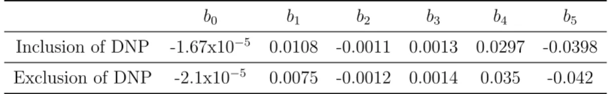
2.1 Best-fit coefficients for functional form given by Eq. (2.85). . . 57

2.2 Normalized root mean square error for estimation of each variable given func-tional fit corresponding to the coefficients listed in Table 2.1. . . 58

3.1 Runtime on Intel Core 2 Duo (2.4GHz) for a range of pressure steps using implementations of the non-adaptive LBM approach and the adaptive LBM algorithm. . . 91

LIST OF FIGURES

2.1 Two-dimensional micro-model in which the solid is represented by black and the regions accessible to fluid flow by white. . . 47

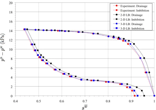
2.2 Pressure-saturation curves obtained from the displacement experiment and the LBM simulations for the porous geometry shown in Figure 2.1. . . 48

2.3 Pressure-saturation equilibrium states computed using the LBM. . . 53

2.4 Fluid distributions for a set of equilibrium states along the simulated primary drainage curve shown in Figure 2.3. . . 54

2.5 Fluid distributions for a set of equilibrium states along the simulated main imbibition curve shown in Figure 2.3. . . 55

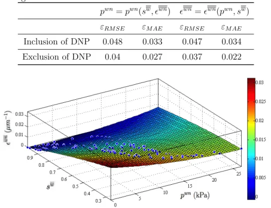
2.6 ✏wn _{as a function of p}wn _{and s}w _{for the case in which DNP is excluded. . . . 58}

2.7 Error in sw _{resulting from the equation of state given by Eq. (2.85) for the}

case in which DNP is excluded. . . 59

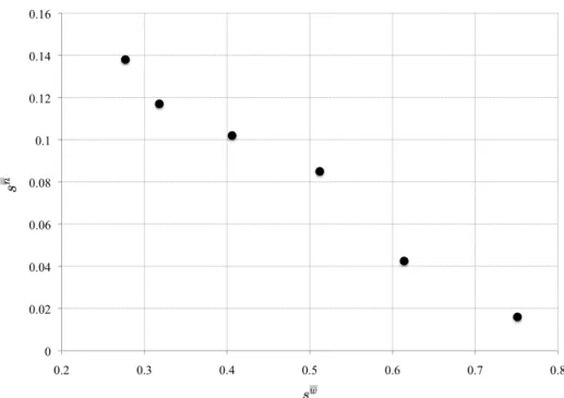
2.8 Maximum disconnected non-wetting phase saturation that can form as a func-tion of the minimum wetting-phase saturafunc-tion state of the system. . . 61

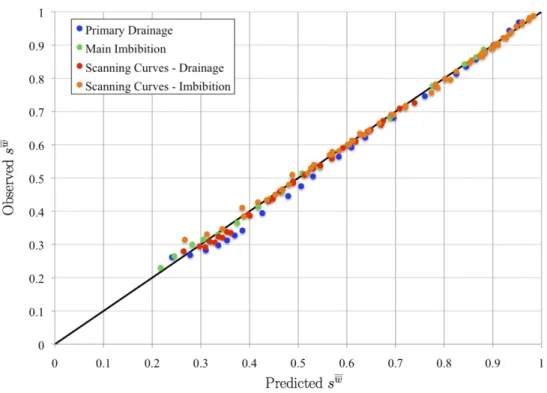
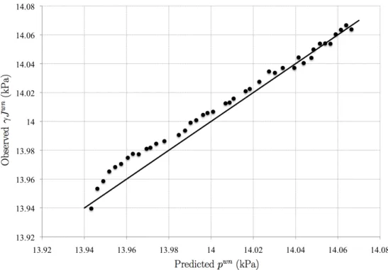
2.9 Observed versus predicted values ofpwn _{for points from a dynamic LBM}

sim-ulation of relaxation to an equilibrium state. . . 63

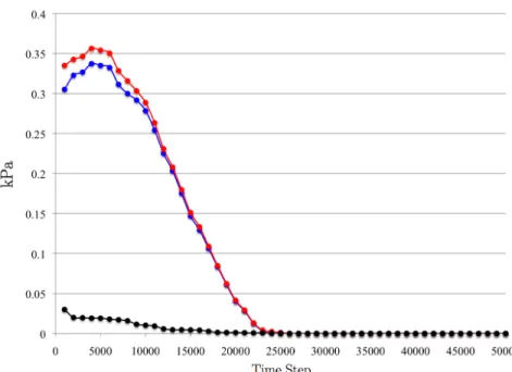
2.10 A comparison of the capillary pressure obtained under dynamic conditions in the simulations and predictions based upon the state equation derived using only equilibrium data. . . 65

3.1 The di↵erence in phase pressures pn _pw _{as a function of the product of the}

interfacial tension wn _{and interfacial curvature J}wn

w as determined using a

series of two-dimensional bubble tests in the absence of a solid phase. . . 81

3.2 Two-dimensional porous media in which the solid is represented by gray and the pore space is represented by white. . . 82

3.3 The phase pressure di↵erence, wetting phase saturation, and capillary pressure values as they evolved in time from one equilibrium state to the next. . . 84

3.4 Adaptive LBM algorithm for two-fluid-phase flow. . . 88

3.5 Pressure-saturation curves obtained from LBM simulations performed using the non-adaptive LBM and the adaptive LBM algorithm. . . 90

3.7 The time evolution of the active fraction of the domain for the equilibrium state simulation depicted in Figure 3.6. . . 94

3.8 The active fraction of the domain as a function of time for an equilibrium state simulation in which a Haines jump occurs. . . 94

3.9 The time evolution of then phase distribution during a Haines jump. . . 95

3.10 Fluid distributions for a set of simulated equilibrium states along the primary drainage curve shown in Figure 3.5. . . 96

3.11 Fluid distributions for a set of simulated equilibrium states along the main imbibition curve shown in Figure 3.5. . . 97

3.12 The initial state of an equilibrium simulation during main imbibition where the red interface identifies thewninterface that is mobile during the simulation. 98

4.1 Two-dimensional porous medium cell in which the solid is represented by black and the regions accessible to fluid flow by white. . . 104

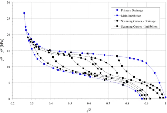
4.2 Primary drainage, main imbibition, and scanning curves obtained from the microfluidic displacement experiment for the porous geometry shown in Fig-ure 4.1. . . 110

4.3 Primary drainage and main imbibition curves obtained from the microfluidic displacement experiment and the LBM simulations for the porous geometry shown in Figure 4.1. . . 110

4.4 The simulated and observed dynamic states between equilibrium states on the primary drainage curve shown in Figure 4.3. . . 111

4.5 The simulated and observed dynamic states between equilibrium states on the main imbibition curve shown in Figure 4.3. . . 112

4.6 Fluid distributions for a set of imaged equilibrium states along the primary drainage curve shown in Figure 4.2. . . 113

4.7 Fluid distributions for a set of imaged equilibrium states along the main im-bibition curve shown in Figure 4.2. . . 113

4.8 The time evolution of the boundary pressures, wetting phase saturation, fluid-fluid interfacial area, and capillary pressure values as the two-fluid-fluid-phase sys-tem relaxes toward equilibrium. . . 115

4.10 The fluid distributions of a two-dimensional slice of a simulated equilibrium state compared to the fluid distributions of an experimental image for the corresponding pressure value. . . 117

4.11 Primary drainage curve as computed from the fluid distributions of a two-dimensional slice of the three-two-dimensional simulated data and the experimen-tal image data. . . 118

4.12 The viscous fingering pattern of a two-dimensional slice of a simulated equi-librium state compared to the viscous fingering pattern of an experimental image for the corresponding capillary pressure value . . . 119

LIST OF ABBREVIATIONS AND SYMBOLS

ACRT averging of conservative equations with rational thermodynamics

CAH chlorinated aliphatic hydrocarbon

CIT classical irreversible thermodynamics

DNAPL dense non-aqueous phase liquid

DNP disconnected non-wetting phase

FLOP floating point operation

LBM lattice Boltzmann method

LNAPL light non-aqueous phase liquid

MAE mean average error

MVA method of volume averging

NAPL non-aqueous phase liquid

PAH polyaromatic hydrocarbon

PCE tetrachlorethylene

PMMC porous medium marching cubes

RAV representative averaging volume

REV representative elementary volume

RMSE root mean square error

TCAT thermodynamically constrained averaging theory

Nomenclature

b entropy body source density

C Green’s deformation tensor,_rXx·(rXx)T

Cs macroscale Green’s deformation tensor, hCsi⌦s,⌦s

Ci Collision operator for the LBM

ˆ

c closure coefficient

cs speed of sound

C gradient of the dimensionless density field

d↵ macroscale rate of strain tensor, [rv↵_{+ (rv}↵₎T_]/2

E internal energy density

E↵ _{macroscale energy of entity ↵ per total volume, hE} ↵i_⌦↵,⌦

E↵

⇤ particular material derivative form of a macroscale entity total energy conservation

equation

Ed set of discrete velocity vectors

ei discrete velocity vector i

f general scalar function

f vector containing discrete distributions for the LBM

Fdk set of discrete distributions

G↵ _{macroscale orientation tensor for↵ interface or common curve,} D_{I I}(n)

↵

E

⌦↵,⌦↵

Gi↵

G↵

⇤ macroscale entity-based body force potential balance equation

g body force per unit mass, acceleration

g↵

i LBM distribution for mass transport of phase↵

h energy source density

h↵ _{macroscale energy source density for entity↵}

I unit tensor

I(n)_↵ unit tensor associated with 3 n-dimensional entity, ↵

I set of entity indices

Ic↵ connected set of indices for entity ↵, =I+c↵[Ic↵

I+

c↵ connected set of indices of dimension higher than entity↵

I_c↵ connected set of indices of dimension lower than entity ↵

If set of fluid-phase indices

II set of interface indices

IP set of phase indices

I/S set of entity indices except the solid phase,s

J first curvature equal to twice the mean curvature

j jacobian

j fluid momentum

ˆ

kwn _{parameter for rate of relaxation of interfacial area}

ˆ kwn

1 parameter for rate of relaxation of interfacial area

k I boundary node on the interfacial region⌦I

M

!↵ microscale transfer rate of mass of entity to entity ↵ per entity extent

!↵

M macroscale transfer rate of mass of entity  to entity ↵ per entity extent

M↵

⇤ macroscale entity mass conservation equation

M transformation matrix

m vector of moments

n↵ unit normal vector outward from boundary of entity ↵

ns interface between n and s phases

P↵

⇤ macroscale entity momentum conservation equation

P pressure, interfacial tension, or common curve lineal tension based upon entity

qualifier

p pressure

p pressure as measured by the pressure transducer

pwn _{capillary pressure of thewninterface}

Q

!↵ general macroscale transfer rate of energy from entity  to entity↵ !↵

Q general macroscale transfer rate of energy from entity  to entity↵

q non-advective energy flux

R radius

ˆ

R closure scalar

r general integration variable

S↵

⇤ macroscale entity entropy balance

s↵ _{saturation of fluid phase↵}

ˆ

S Diagonal matrix of relaxation rates

T transport theorem

T

!↵ general microscale transfer rate of momentum from entity  to entity ↵

!↵

T general macroscale transfer rate of momentum from entity  to entity ↵

Ts

⇤ macroscale Euler equation for a solid

T↵

⇤ macroscale Euler equation for an entity

Ts

G⇤ body source potential of a solid phase

T↵

G⇤ entity body source potential

t time

t timestep

t stress tensor

t↵ _{macroscale stress tensor for entity↵}

V set of variables

W weighting function for averaging

wxx free parameter in the MRT scheme

wi weight for the LBM

w wetting phase

wn interface between wand n phases

wns common curve at boundary ofwn,ws, and nsinterfaces

ws interface between wand s phases

w velocity of a domain boundary

wwn vector velocity of normal component ofwn interface, vwn·nwnw

wh width of the halo around the interfacial region⌦I

X position vector in a solid in the initial state

Xk set of neighboring lattice sites to sitexk

x position vector

sZd regular lattice space ind dimensions

Greek Symbols

↵ entity index

entity index

t number of time steps of the LBM in the Adaptive LBM Algorithm

interfacial or surface tension; common curve lineal tension

✏ porosity

✏↵ _{specific entity measure,h1i}

⌦↵,⌦

"w termination condition in the Adaptive LBM Algorithm

⇣ parameter controlling interfacial width in LBM

⌘ entropy density

⌘↵ _{macroscale entropy of entity ↵ per volume, h⌘} ↵i⌦↵,⌦

✓ temperature

✓↵ entropy weighted macroscale temperature of entity ↵, h✓↵i⌦↵,⌦↵,⌘↵

wns

G macroscale geodesic curvature

wns

N macroscale normal curvature

w termination condition in the Adaptive LBM Algorithm

⇤ entropy production rate

⇤↵ _{macroscale entropy production rate associated with entity ↵}

µ chemical potential

⇢ mass density

LBM parameter used to control the interfacial tension

solid-phase stress tensor

dimensionless density field

s solid phase value of dimensionless density field

!↵

general macroscale transfer of entropy from entity to entity ↵

'ws,wn _{macroscale measure of contact angle}

' non-advective entropy flux

'↵ _{macroscale non-advective entropy flux associated with entity↵}

'_ws,wn microscale contact angle



↵ fraction of boundary of entity ↵ in contact with entity ,h1i⌦,⌦↵

body force potential density

↵ _{entity-based macroscale body force potential density}

body force potential per unit mass

↵, _{macroscale average of body force potential density}

⌦ averaging domain

⌦↵ domain of entity↵

Superscripts

eq equilibrium value

n macroscale non-wetting phase qualifier

ns macroscale qualifier for interface betweenn and s phases

s macroscale solid-phase qualifier

T transpose

w macroscale wetting-phase qualifier

wn macroscale qualifier for interface betweenw and n phases

wns macroscale qualifier for common curve where wn, ws and ns interfaces meet

ws macroscale qualifier for interface betweenw and s phases

↵ macroscale entity qualifier

↵ intrinsic average over entity↵ or macroscale property of entity ↵

↵ mass average over entity↵

↵ uniquely defined average over ↵

above a superscript refers to a density weighted macroscale average

above a superscript refers to a uniquely defined macroscale average

0 vector tangent to a surface

00 vector tangent to a common curve

Subscripts

eq equilibrium value

E associated with the total energy conservation equation

eq equilibrium

M associated with the mass conservation equation

n microscale non-wetting-phase qualifier

ns microscale qualifier for interface betweenn and s phases

P associated with the momentum conservation equation

s microscale solid-phase qualifier

ss refers to the total boundary of the s phase

T total

T associated with the thermodynamic equation

TG associated with the derivative of potential energy equation

w microscale wetting-phase qualifier

wn microscale qualifier for interface betweenw and n phases

wns microscale qualifier for common curve wherewn, ws and nsinterfaces meet

ws microscale qualifier for interface betweenw and s phases

↵ microscale entity qualifier

↵↵ refers to the total boundary of entity ↵

Other Mathematical Symbols

D↵/Dt material derivative with microscale velocityv↵

D↵_{/Dt material derivative with macroscale velocityv}↵

D00s_{/Dt material derivative on a curve where the macroscale solid is employed}

@0_{/@t partial time derivative at a point fixed on a surface}

@00/@t partial time derivative at a point fixed on a common curve

@(n)_{/@t partial time derivative at a point fixed on 3 n-dimensional entity}

r0 _{microscale surficial del operator}

r00 _{microscale common curve del operator}

r(n) _{microscale del operator for a 3 n-dimensional entity where (n) is the number of}

primes

rX gradient operator with respect to X coordinates

rx gradient operator with respect to macroscale xcoordinates

(n) denotes the number of primes that should appear

ˆ a parameter defined at the scale indicated by the subscript or superscript

hf↵i⌦ ,⌦ ,W = ✓ _R

⌦

W f↵dr

◆

/

✓_R

⌦

Wdr

◆

, average of microscale property f↵

f_↵ =_hf↵i_{⌦ ,⌦}

f↵ _=hf

↵i_{⌦↵,⌦↵}, intrinsic average

f_↵ =hf↵i_{⌦ ,⌦ ,⇢↵}, general density-weighted average

f↵ _=hf

CHAPTER 1 INTRODUCTION

1.1 Multiphase Flow in Porous Media

A porous medium system contains a continuous connected solid phase and a connected pore

space that spans the length scale of the system and admits the simultaneous flow of one

or more fluids. When the pore space in such a system can be occupied by more than one

immiscible fluid (e.g., water, gas, organic solvent, petroleum liquid), the system is commonly

referred to as a multiphase porous medium system. Porous medium systems occur routinely

in both natural and engineered environments for a wide range of important applications, such

as groundwater supply, contaminant remediation, carbon sequestration, hydraulic fracturing,

and hydrogen fuel cells.

The contamination of groundwater, a significant source of drinking water, is a serious

health and environmental problem in many areas of the United States. Groundwater

contam-ination is generally the result of human activities such as waste-disposal practices, runo↵from

agriculture, accidental spills and leaking underground storage tanks that contain protroleum

products [24, 83]. Contaminants associated with accidental spills and leaking underground

storage tanks are often released as non-aqueous phase liquids (NAPLs). When introduced

into the subsurface, NAPLs form a separate, potentially mobile phase whose migration is

governed by gravitational, buoyant, viscous, and capillary forces. [16, 18, 43]. NAPLs are

density, LNAPLs tend to migrate to the capillary fringe of the water table whereas DNAPLs

can to travel deep into the saturated zone. LNAPLs are commonly released into the

environ-ment via the production, use, and disposal of many products associated with the petroleum

and gasoline industries, and include toluene, ethylbenzene, octane, decane, and benzene, a

known carcinogen. The presence of DNAPLs in the subsurface is typically associated with

in-dustrial activities such as degreasing, metal stripping, chemical manufacturing, and pesticide

production [126]. Common chemicals associated with DNAPLs include chlorinated aliphatic

hydrocarbons (CAHs), such as tetrachlorethylene (PCE) and trichloroethylene (TCE), and

polyaromatic hydrocarbons (PAHs). Once the source of the NAPL is cut o↵ or depleted,

continuous NAPL phase may become numerous disconnected features in the pores. These

features are held in the pore space by capillary forces and can act as continual sources of

contamination for decades or even centuries [133, 135]. In order to e↵ectively develop and

assess remediation strategies, models describing the migration and entrapment of NAPLs in

the subsurface are necessary.

Multiphase flow also arises within hydraulic fracturing operations. Due to an increase

in energy demands and economic benefits, the use of hydraulic fracturing to extract natural

gas from organic-rich shales is expanding [90]. Hydraulic fracturing is the process of drilling

and injecting fluid into the ground at a high pressure in order to fracture shale rocks. The

objective of hydraulic fracturing is to create a highly conductive fracture system that will

allow flow through the shale rock to the production well used to extract natural gas from

the subsurface. Hydraulic fracturing fluids are used to initiate and expand fractures, as well

as to transport proppant into fractures within the shale rock. Proppants are sand or other

transport and entrapment of proppant into a fracture is highly dependent on the viscosity

of the fracturing fluid [120]. There are over 750 di↵erent chemicals used in fracturing fluids

[121]. A majority of these chemicals, such as citric acid and guar gum, pose no known

health risk, but others, such as benzene and lead, are known carcinogens. After fracturing of

the shale occurs, the injection of fracturing fluid is stopped and a portion of the fracturing

fluids flow back to the surface. During flow back, multiphase flow of gas and fracture fluid

occurs in the created fracture and the gas reservoir. When simultaneous flow of di↵erent

phases occurs in a hydraulic fracture, factors such as relative permeability, capillary pressure,

and wettability inside the fracture and the reservoir could potentially be important in the

fracturing fluid behavior and long term gas production in the gas reservoir. Due to the

uncertainity surrounding the behavior of fracturing fluids within the subsurface, the potential

impacts of hydraulic fracturing operations on groundwater resources is becoming a concern

[125]. Multiphase models describing the transport and fate of injected fracturing fluids under

conditions of high pressure and temperature are necessary to adequately examine current

hydraulic fracturing technologies.

1.2 Modeling Multiphase Flow

Multiphase flow in porous media is modeled on several di↵erent length scales (molecular

scale, microscale, macroscale, and megascale), each of which is inherently related to the

other. The two scales of interest in this work are the microscale and the macroscale. At

the microscale, the morphology and topology of the pore space and phase distributions are

known. At the macroscale, the details of the system at the microscale are unknown. Since

used in characterizing porous medium systems, such as the fractional volume of the porous

media occupied by each phase, porosity or the volume of pore space within the total volume,

and interfacial area between phases per volume. In order to identify and characterize these

properties, the characteristic length at the macroscale must be large enough that the volume

fractions will not be e↵ected by small changes in the length scale. Therefore, upscaling

from the microscale to the macroscale is commonly done by averaging over a representative

elementary volume (REV), a volume that is smaller than the domain of the system, but that

is large enough to permit a meaningful statistical average.

Due to the fact that porous medium systems are usually understood more completely

at the microscale, it seems logical to develop macroscale flow models by establishing a

con-nection to the microscale physics. However, traditional macroscopic porous medium models

for multiphase flow are often obtained by combining empirical relationships with standard

continuum conservation equations for mass written at the macroscale, therefore ignoring the

microscale physics. For example, a two-fluid-phase porous medium system is often modeled

using Darcy’s law, a form of the mass conservation equation, where the interaction between

the phases is accounted for by introducing relative permeability and assuming the di↵erence

in pressure between the two fluids is related by capillary pressure [40]. In order to close

this model, an empirical relationship between capillary pressure, saturation, and

perme-ability is introduced. The many functional forms of the capillary pressure, saturation, and

permeability relationship that have been reported in the literature demonstrate hysteretic

behavior, implying other variables are needed to fully specify the state of the multiphase

system [19, 23, 76]. Like the multiphase model discussed here, many standard macroscopic

foun-dation and misrepresent the underlying microscale physics. Recent theoretical work aims

to improve traditional modeling approaches by basing macroscopic models on microscale

precursors.

The thermodynamically constrained averaging theory (TCAT) provides a means for

ob-taining macroscopic models from microscopic models via averaging schemes [52, 56]. At the

microscale, conservation equations are combined with thermodynamics, constitutive laws

and simplifying assumptions to obtain a microscopic description of the system. To obtain a

macroscopic model, the thermodynamics and conservation equations are averaged from the

microscale. This ensures that all macroscopic variables are rigorously defined in terms of

more familiar microscale variables, eliminating any ambiguity with respect to these variables.

The macroscopic equations are then combined with simplifying assumptions and constitutive

relationships, which must be determined in order to obtain a closed model. Closed models

are needed both to facilitate a solution of an equation set and to allow for validation of

TCAT models by comparison with system behavior observed at the corresponding scale.

Advances in microscale computational and experimental methods have helped guide the

development of closed form models. Many traditional fluid mechanics approaches are not

well suited to deal with the complexity of flows in porous media. The lattice Boltzmann

method (LBM) has emerged as a leading alternative to traditional approaches due to the

simplicity by which fluid and solid interfaces are treated. In addition to LBMs designed

to model multiphase flows, algorithms have also been constructed to model a wide range of

physical processes including di↵usion [45, 77], dissolution [25, 124], phase transitions [2, 107],

and reactive transport [37, 68].

can be studied experimentally using micro-model methods based upon image analysis.

Two-dimensional micro-models are synthetic porous media that provide valuable insights into

important pore-scale mechanisms of multiphase flow in porous media systems [27, 28, 69].

Most micro-models are etched as natural porous substrates to imitate natural processes or as

simple pore networks of circular pore bodies to quantify basic transport phenomena. To allow

for the microscopic analysis of fluid flow, micro-models are created out of transparent material

(glass, silicon, or polymers) and imaged under a microscope. Due to their design,

micro-models have also been used to visualize and quantify colloid transport and filtration [11] and

investigate chemical reactions that take place in the subsurface environment [70, 132].

1.3 Research Objectives

The research presented here is focused on advancing the fundamental understanding of

two-fluid-phase porous medium systems using theoretical, computational, and experimental

ap-proaches. Recent advancements in both methods development and application of the LBM

will be presented. Results will be shown for both the equilibrium state and dynamics of

two-fluid-phase flow.

The specific objectives for this research are as follows:

1. Formulate a model for two-fluid-phase flow in porous medium systems based on the

TCAT theory.

2. Construct computational and experimental methods capable of capturing the

micro-scale physics needed to guide the development of closed models in conjuction with the

3. Investigate the validity of capillary pressure approximations used to describe

two-fluid-phase porous medium systems and develop functional forms based on state variables

by applying the LBM and comparing results to experimental data.

4. Advance existing LBM algorithms in order to account for the relatively slow process

in which fluid interfaces relax to their equilibrium state in a two-fluid-phase porous

medium system.

The objectives of this work are accomplished through 3 specific contributions, which are in

CHAPTER 2

MULTISCALE MODELING OF POROUS MEDIUM SYSTEMS 1

2.1 Background

The use of computers over the last 60 years for simulating subsurface flow problems has

pro-vided an impressive ever-expanding ability to model processes at a high resolution. Whereas

in the 1960’s a computational grid with 500 fixed nodes would have pushed the boundaries

of computer power [105], simulations today involve millions of spatial grid points and

adap-tive meshes [71, 101]. The availability of this power for solving the equations that describe

physical and chemical processes in porous media is wasted, however, if the equations being

used to describe the systems are inadequate. Most assuredly, the ability to solve equations

that are posed has been vastly improved. Unfortunately, the equations that are being solved

have not developed to the same degree.

For example, the primary equation for describing momentum transport of fluids in porous

media is Darcy’s Law, a correlation of data from a highly idealized set of experiments (e.g.,

homogeneous medium, single-fluid phase, steady state) in 1856 [17, 35, 36]. The results

of these experiments have been presumed to apply to transient, multiphase, flows in

het-erogeneous systems at di↵erent scales. This extension of the experiment to systems clearly

beyond their scope has resulted in equations with ill-defined and poorly understood variables.

A clear path for rigorously extending the form of Darcy’s equation to flows well beyond those

considered by Darcy, such as high-velocity flow and flows with cross-coupling between the

fluid phases, does not exist. Furthermore, inclusion of physical phenomena such as capillary

pressure, contact angles, and evolution of interfaces between phases has been a heuristic

ef-fort justified somewhat by dabbling in physical understanding rather than a comprehensive

rigorous derivation of equations that describe the processes [e.g., 61, 87, 94].

Averaging of equations from the microscale to a larger scale is one general approach

that has been employed in an e↵ort to obtain equations that have a firm theoretical basis.

Underlying averaging theory is the mathematical theorems that allow transformation of the

scale of equations. Theorems for transformation of conservation equations for phases have

been employed for almost fifty years [5, 8, 109, 129]. Theorems that allow averaging of

equations for interfaces between phases and for common curves where three interfaces meet

were developed subsequently [49, 51] and the forms of all these equations were subsequently

unified [55]. Four principal variants of averaging theory that make use of these theorems

have been employed. The first emphasizes averaging of microscale conservation equations for

phases and then makes heuristic arguments to close the equation system [e.g., 13, 57, 129].

A second approach pioneered by Whitaker and employed by adherents to this approach

is commonly referred to as the method of volume averaging (MVA). Applications of MVA

typically make use of averaging theorems applied to conservation equations for phases only.

This approach begins with closed microscale equations, which are then averaged to a larger

scale. The new terms that arise are closed by derivation of closure equations solved for a

periodic unit cell and the solution of closure variables to map from the smaller scale to the

The third approach makes use of averaging of conservation equations in conjunction

with rational thermodynamics (ACRT). ACRT averages equations for phases, interfaces, and

common curves. Then based on a set of axioms concerning system behavior, thermodynamic

relations are obtained directly at the larger scale, and the equation set is closed based on

exploitation of an entropy inequality [e.g., 14, 58, 60, 115].

These preceding methods have shortcomings primarily in that the first two methods do

not account for interface dynamics and require assumptions about the forms for deviations

between microscale and larger scale values. The approaches make very limited use of

ther-modynamic information. ACRT su↵ers in that the larger scale thermodynamic relations in

fact are expressed in terms of quantities that are not based on fundamental thermodynamic

variables [9, 75, 79, 123]. Additionally, these models have been abused by using erroneous

clo-sure conditions for the interface stress tensor and the interface dynamics [e.g., 88, 89]. Thus,

complete and correct models based on averaged conservation equations, thermodynamics,

and phase distribution kinematics are missing.

In an e↵ort to overcome the problems of these earlier methods, a fourth method, referred

to as thermodynamically constrained averaging theory (TCAT) has been formulated. This

method is the basis of this contribution. Here we outline the elements of TCAT and show

how it can be used to obtain model equations that overcome many theoretical difficulties.

2.2 Introduction

Conservation equations and thermodynamic relations applicable to porous medium systems

above the microscale, where a point refers to the averaged conditions in some representative

averaging region. We will call this larger scale the macroscale. The thermodynamically

con-strained averaging theory (TCAT) has been developed to formulate macroscale models such

that all variables are expressed explicitly in terms of microscale precursors [52, 56]. TCAT

also assures consistency with the second law of thermodynamics. It has been shown that

use of the TCAT procedure leads to the occurrence of variables such as volume fractions,

interfacial tensions, and density of interfacial area between the fluid and solid phases for the

case of single-fluid porous medium systems. For multifluid systems, common curve lengths

per volume, interfacial tensions, curvatures, and contact angles also arise naturally in the

for-mulation [66]. On physical grounds, these variables can be argued to be of importance; their

magnitudes relate to possibilities for interactions and exchanges between phases. However,

these variables do not appear explicitly in traditional porous medium models.

Despite the theoretical appeal of TCAT models, a problem remains: solvable models

require the explicit identification of closure relations that have only been specified in general

functional forms by the theoretical work advanced to date. The constitutive relations

em-ployed for a particular system must be consistent with the general forms inferred and also

clearly stipulated and parameterized. Closed models are needed both to facilitate solution

of an equation set and to allow for validation of TCAT models by comparison with system

behavior observed at the corresponding scale.

In recent years, some needed closed forms have been motivated by small scale

experimen-tal and computational methods. Of particular interest here is the high-resolution microscale

modeling approach known as the Lattice Boltzmann method (LBM). This method can be

the pores of a porous medium system and and also the macroscale variables that can be

obtained as integrated forms of the microscale variables. These macroscale variables can be

employed in posited general forms of closure relations [42, 59, 93, 116]. Computational

ex-periments thus provide a basis for the development of closed models making use of equations

developed using the TCAT procedure. Because TCAT models are new, multiscale modeling

of specific forms of TCAT closure relations has not yet been completed for many theorized

model forms.

In this chapter, we examine a TCAT model for two-fluid-phase flow in a porous medium

system. In Section 2.3, we provide the theoretical elements that are combined to establish the

TCAT approach. In Section 2.4 we propose a set of closed equations that describes

two-fluid-phase flow in a porous medium. For this set to be solvable, values or functional forms of some

coefficients and equations of state must be specified. In Section 2.5, we discuss how knowledge

of the smaller scale system behavior, obtained through complementary experimental and

LBM studies, can provide insights for specification of the needed forms and coefficients.

Section 3.2 provides details concerning the formulation, verification, and validation of the

LBM approach used to simulate two-fluid-phase flow in a porous medium system. The

resultant model is used to investigate various aspects of of the flow system that the TCAT

model suggests warrant attention, such as an appropriate formulation of capillary pressure.

The need to obtain information about geometric features of the porous medium system,

such as the curvature of interfaces between phases and the extent of those interfaces, is

discussed in Section 2.7. In Section 2.8 specific closure relations for a two-fluid-phase system

are obtained from analysis of LBM simulations. This serves as an illustration of how robust

with computer simulation for a range of phenomena.

2.3 Theory

TCAT is a systematic procedure for changing the scale of conservation, balance, and

ther-modynamic equations from the microscale to a larger scale. For use in porous media, the

TCAT method involves averaging over a representative averaging volume (RAV) to obtain

equations for phases, interfaces between phases, common curves, and common points, which

are referred to generically as entities. The method has been developed by considering each of

these entities separately. Here, we will make use of the similarities of the equations and

aver-aging theorems for each of the di↵erent entity types to develop the equations. The following

six subsections present the following TCAT components: averaging theorems, conservation

equations, entropy balance, thermodynamic equations, evolution equations, and the entropy

inequality. The full details of these equations and the procedures used to manipulate them

can be found in [56]. Here, we emphasize the equations that are particularly useful in

mac-roscale porous medium flow modeling. These results form the bases for model formulation

and closure considerations, which are considered subsequently.

2.3.1 Averaging Theorems

For porous medium analysis, it is not possible to model large systems at a microscale where

the flow profile within the pores is described. Neither is it always informative to model the

system at a megascale where only an average value of a quantity within the full system is

determined. As a compromise between these two extremes, it is important to be able to

as the macroscale, where a filtered variability of quantities in the system is used. At the

microscale, the phases within a system are visualized as being juxtaposed and separated by

interfaces. At a microscale location, a point lies within a single phase or on an interface or

a common curve. From a macroscale perspective, all phases, interfaces, and common curves

may be present at a location with each having a geometric density. A phase has a volume

fraction measure, an interface has an interfacial area per volume measure, and a common

curve has a length per volume measure. A similar density can be developed for common

points, which do not occur in the systems considered in this chapter.

The conservation and balance equations that describe a system are most easily formulated

directly in terms of microscale quantities. To transform the microscale equations to the

macroscale, mathematical relations are needed. These have the e↵ect of changing averages of

derivatives of microscale quantities into derivatives of macroscale quantities. These theorems

[5, 49–51, 55, 64, 78, 86, 109, 128] are most readily applied when the length scales of the

microscale and macroscale are widely separated. Microscale phase conservation equations

are three-dimensional transient forms. Interface conservation equations are two-dimensional

at the microscale. Common curves and common points are, respectively, one- and

zero-dimensional at the microscale. On transformation to the macroscale, all these equations

become three-dimensional as the properties of interest vary in space regardless of the type

of entity to which they belong.

operators according to

⌦

r(n)·f↵

↵

⌦↵,⌦ =r·

D

I(n)_{↵ ·}f↵

E

⌦↵,⌦

D⇣

r(n)·I(n)_↵ ⌘_·f↵

E

⌦↵,⌦

+ X

2Ic↵

hn↵·f↵i⌦,⌦ (2.1)

and

⌦

r(n)_f

↵

↵

⌦↵,⌦ =r·

D

I(n)

↵ f↵

E

⌦↵,⌦

D⇣

r(n)_·I(n)

↵ ⌘ f↵ E ⌦↵,⌦ + X

2Ic↵

hn↵f↵i_⌦,⌦ , (2.2)

where (n) is the number of primes that appear in the superscript, and the integration domain

is of dimensionality 3 n. Thus, for example, for a surface of dimensionality 2, (n) = (1),

so the microscale surface gradient operator,r0_{, uses a single 0to indicate that it is a surface}

operator. For a phase, n = 0, and I(0)

↵ = I. For a common point, n = 3 and I(3)↵ =0. Note

that all variables and operators are defined in the nomenclature section.

In addition to the spatial averaging theorems, a temporal averaging theorem is employed

that relates the spatial average of a time derivative of a function to the time derivative of

the spatial average of the function. This theorem is stated

⌧ @(n)_f

↵

@t _⌦↵,⌦ =

@

@thf↵i⌦↵,⌦ +r·

D⇣

I I(n)_↵ ⌘_·v↵f↵

E

⌦↵,⌦

+D_r(n)_·I(n)

↵ ·v↵f↵

E

⌦↵,⌦

X

2Ic↵

hn↵·vf↵i_⌦,⌦ , (2.3)

where (n) is the number of primes that appear in the superscript, and the integration domain,

⌦↵, is of dimensionality 3 n. Eqs. (2.1) and (2.3) are the primary averaging theorems that

and common points to their macroscale forms.

2.3.2 Conservation and Balance Equations

The conservation equations at the macroscale can all be derived from the microscale total

energy equation by application of the averaging theorems followed by the restriction that the

equation obtained must apply in any inertial coordinate system. In the development here,

we will not consider species transport or interphase mass transfer of individual species. We

state the microscale total energy equation for entity ↵ as

E↵ :=

@(n) @t

⇣

E↵+⇢↵

v↵·v↵

2 + ↵

⌘

+_r(n)_·h⇣E↵+⇢↵

v↵·v↵

2 + ↵

⌘ v↵

i

h_↵ ⇢↵

@(n)

↵

@t ⇢↵g↵·

⇣

I I(n)

↵

⌘

·v↵

X

2I+c↵

✓

E

⇢

+ v·v

2 + 

◆

M

!↵+v·T!↵+_Q_!↵

r(n)_·⇣_I(n)

↵ ·t↵·v↵+I(n)↵ ·q↵

⌘

= 0 for ↵2I;n = 3 dim ↵ , (2.4)

where the summation term in this equation accounts for exchanges with entities of higher

dimensionality.

This equation is averaged to the macroscale using the operator h·i⌦↵,⌦. After application

of the averaging theorems Eqs. (2.1) and (2.3), the macroscale energy equation that results

is

E↵ _:= @

@t



E↵+✏↵⇢↵ ✓

v↵_·v↵

2 +K

↵

E ◆

+ ↵

+r·

⇢

E↵+✏↵⇢↵ ✓

v↵_·v↵

2 +K

↵

E ◆

✏↵h↵ X

2Ic↵

!↵

M E↵,+v

↵,_·v↵,

2 +K

↵,

E + ↵, !

X

2Ic↵

!↵

T _·v↵, X 2Ic↵

!↵

Q

r·⇣✏↵t↵_·v↵+✏↵q↵+✏↵q↵_g⌘ ⌧

⇢↵

@(n)

↵

@t _⌦↵,⌦

D ⇢↵v↵·

⇣

I I(n)

↵

⌘

·g↵

E

⌦↵,⌦

= 0 for ↵2I;n= 3 dim ↵. (2.5)

The notation used in this equation is designed to precisely indicate the macroscale quantities

(with superscripts), particular kinds of averages (spatial average with no overbar on the

superscript, mass density weighted with a single overbar on the superscript, specially defined

with a double overbar on the superscript), an exchange terms between entities (with a super

arrow indicating the transfer from one entity to the other). The definitions arise naturally

in the averaging process, and the expressions in terms of microscale variables appear in the

nomenclature or in far greater detail in [56]. It is useful to rewrite the first two terms in Eq.

(2.5) making use of the material derivative operator to obtain

E↵

⇤ :=

D↵

Dt



E↵+✏↵⇢↵ ✓

v↵_·v↵

2 +K

↵ E ◆ + ↵ + 

E↵+✏↵⇢↵ ✓

v↵_·v↵

2 +K

↵

E ◆

+ ↵ I:d↵

✏↵h↵ X

2Ic↵

!↵

M E↵,+v

↵,_·v↵,

2 +K

↵,

E +

↵,

!

X

2Ic↵

!↵

T _·v↵, X

2Ic↵

!↵

Q

r·⇣✏↵t↵

·v↵+✏↵q↵+✏↵q↵_g⌘ ⌧

⇢↵

@(n)

↵

@t _⌦↵,⌦

D ⇢↵v↵·

⇣

I I(n)_↵ ⌘_·g_↵E ⌦↵,⌦

This energy equation must apply in any inertial reference coordinate system. We can

replace v↵ by v↵+C, where Cis an arbitrary constant velocity vector, and Eq. (2.6) will

still apply. After making this substitution, collection of terms that multiply Cresults in an

equation of the form

E↵

⇤ +C·P↵⇤ +

C_·C

2 M

↵

⇤ = 0. (2.7)

Because C is arbitrary, selection of C = 0 confirms that Eq. (2.6) still applies. If C

is orthogonal to the terms collected to form P↵

⇤, then Eq. (2.7) requires that M↵⇤ = 0.

Therefore, we must also have _P↵_⇤ = 0, since Eq. (2.7) must hold for all constant C. The

group of terms that comprise _P↵_⇤ is the momentum equation as follows:

P↵

⇤ :=

D↵

Dt

⇣

✏↵⇢↵v↵⌘+✏↵⇢↵v↵I:d↵ ✏↵⇢↵g↵ X

2Ic↵

!↵

M v↵, X

2Ic↵

!↵

T _r·⇣✏↵t↵⌘=0 for ↵₂I. (2.8)

The elements of M↵

⇤ constitute the mass conservation equation for entity ↵, which can be

written as

M↵⇤ :=

D↵⇣_✏↵_⇢↵⌘

Dt +✏

↵_⇢↵_I:d↵ X 2Ic↵

!↵

M = 0 for ↵₂I. (2.9)

For two-fluid-phase flow, we note that the set of entities is the phases, interfaces, and

common curve such that the index set is

As an example of the connected sets, for the wninterface,

I+_c↵wn=_{w, n_} (2.11)

and

I_c↵wn={wns} (2.12)

We are considering the connected set of the solid phase to include the common curve.

2.3.3 Entropy Balance

In addition to the conservation equations, an entropy balance equation may be formulated

for each entity. The microscale equation denoted as _S↵ is written

S↵ :=@

(n)_⌘

↵

@t +r

(n)_·(⌘

↵v↵) b↵

X

2I+c↵

⌘

⇢

M

!↵ r

(n)_·⇣_I(n)

↵ ·'↵

⌘

=⇤↵

for↵ 2I;n = 3 dim ↵. (2.13)

Application of the averaging theorems Eqs. (2.1) and (2.3) to this equation yields the

macroscale entropy balance,

S↵ := @⌘

↵

@t +r·

⇣

⌘↵v↵⌘ ✏↵b↵ X

2Ic↵

!↵

M ⌘↵,

X

2Ic↵

!↵

As with the conservation equations, it will prove convenient to write this equation in terms

of the material derivative such that we have

S↵

⇤ :=

D↵_⌘↵

Dt +⌘

↵_I:d↵

✏↵b↵ X

2Ic↵

!↵

M ⌘↵, X

2Ic↵

!↵

r·⇣✏↵'↵⌘=⇤↵

for ↵2I. (2.15)

We observe that the quantities that appear in this balance equation do not appear in the

conservation equations. To make use of this equation in conjunction with those equations,

two steps are taken. First, the inter-entity exchange terms will drop out if one sums the

entropy balance equation over all entities. This gives us

X

↵2I

S⇤↵ =

X

↵2I "

D↵_⌘↵

Dt +⌘

↵_I:d↵ _✏↵_b↵

r·⇣✏↵'↵⌘ #

= X

↵2I

⇤↵ . (2.16)

From the second law of thermodynamics, we know that entropy generation due to irreversible

processes is non-negative. Therefore, we know that

X

↵2I

⇤↵ 0. (2.17)

The second step in making the entropy inequality helpful in conjunction with the

con-servation equations is the postulation of a thermodynamic formalism that relates entropy to

2.3.4 Thermodynamic Formalism

The simplest thermodynamic formulation that can be employed is classical irreversible

ther-modynamics (CIT) [9, 22, 38]. We will use this formalism here because of its simplicity and

the fact that it indeed describes the thermodynamic behavior of many important systems.

The approach employed is to make use of the known thermodynamic relations at the

mic-roscale and then average them to the macmic-roscale. By using this approach we ensure that

all thermodynamic quantities are well-defined at the macroscale and that thermodynamic

information is transferred consistently between scales. The thermodynamic formalism can

be developed using a common notation for all entities except the solid. Here, we assume

that the solid is elastic, and we provide the thermodynamic relations consistent with that

specification.

Classical thermodynamics provides thermodynamic properties of equilibrium systems.

Using the CIT approach, we make use of a local equilibrium assumption such that the

thermodynamic relations are considered to apply at each point in the system even though

the properties that are constant when the system is at equilibrium have spatial and temporal

variation. It is important to note that the local equilibrium assumption is enforced at the

microscale but is not imposed separately at a larger scale when the larger scale equations

are obtained by averaging the smaller scale thermodynamic relations. The impact and

importance of non-local equilibrium at the larger scale in the thermodynamic relations is

obtained through the averaging process that requires consistency between scales.

the Euler form of the energy equation per region of the entity written as:

E↵ =✓↵⌘↵+µ↵⇢↵ P↵ for ↵2I/S . (2.18)

In this equation, P↵ = p↵ is pressure when ↵ denotes a fluid phase, P↵ = ↵ for an

interface where ↵ is the interfacial tension, and P↵ = ↵ for a common curve where ↵ is

the curvilinear tension of the curve. The derivative of this equation may be written

d(n)_E

↵=✓↵d(n)⌘↵+µ↵d(n)⇢↵ for ↵ 2I/S , (2.19)

where d is a di↵erential operator, and the superscript (n) constrains the di↵erentiation to

remain at fixed entity coordinates when ↵ is of dimensionality 3 n.

With d(n) _{replaced by @}(n)_{/@t in Eq. (2.19), averaging theorem Eq. (2.3) can be applied}

to obtain a macroscale thermodynamic equation involving the time derivative. If d(n) _is

replaced by the gradient operator, _r(n) _{in Eq. (2.19), the spatial averaging theorem, Eq.}

(2.2), can be used to obtain an expression for the macroscale gradient of energy. Then

summation of these two results after dotting the gradient expression with v↵ _{yields the}

averaged form of the thermodynamic relation given by

T⇤↵ :=

D↵_E↵

Dt ✓

↵D↵⌘↵

Dt µ

↵D↵(✏↵⇢↵)

Dt

+ X

2Ic↵

⌦

n↵· v vs P↵

↵ ⌦,⌦

+

* ⌘↵

D(n)s_(✓

↵ ✓↵) Dt + ⌦↵,⌦ + ⌧ ⇢↵

D(n)s_(µ

↵ µ↵)



⌘↵r✓↵ r·DI(n)_↵ P↵

E

⌦↵,⌦

+✏↵⇢↵rµ↵ · v↵ vs

r·D⇣I I(n)

↵

⌘

· v↵ v↵ P↵

E

⌦↵,⌦

D⇣

I I(n)

↵

⌘

P↵

E

⌦↵,⌦

:d↵

D

r(n)·I(n)

↵ · v↵ vs P↵

E

⌦↵,⌦

+D⌘↵ v↵ vs ·

⇣

I I(n)

↵

⌘E

⌦↵,⌦·r

✓↵

+D⇢↵ v↵ vs ·

⇣

I I(n)_↵ ⌘E

⌦↵,⌦·r

µ↵ = 0 for ↵₂I/S . (2.20)

We emphasize that this expression makes use of the local equilibrium approximation at the

microscale but does not require this condition to hold at the macroscale.

Although it is not a thermodynamic condition, the equation for the rate of change of

the gravitational potential is handled similarly to the thermodynamic condition. Because

↵ =⇢↵ ↵, the derivative of this expression is

d(n) ↵ ↵d(n)⇢↵ ⇢↵d(n) ↵ = 0 for ↵2I. (2.21)

The di↵erential d(n) _{may be replaced, successively, by the partial time derivative and}

gra-dient operators with the averaging theorems applied to the resulting equations. Then if the

resulting equation in terms of the gradient is dotted with v↵ _{and added to the partial time}

derivative equation, the result is

TG↵⇤ :=

D↵ ↵

Dt

↵D↵(✏↵⇢↵)

Dt

⌧ ⇢↵

D(n)s ↵

Dt _⌦↵,⌦ ✏

↵_⇢↵

r ↵· v↵ vs

+D⇢↵ v↵ vs ·

⇣

I I(n)_↵ ⌘E

⌦↵,⌦·r

This equation added to Eq. (2.20) provides a relation for the rate of change of macroscale

internal plus potential energy for fluid phases, interfaces, and the common curve.

A potentially fertile area for additional research is the representation of solid phases at

the macroscale. Here, we adopt a relatively simple model of the solid as an elastic material,

which can be formulated as

Es =✓s⌘s+ s:

Cs

js

+µs⇢s , (2.23)

where s is a stress tensor, Cs is Green’s deformation tensor, and js is the Jacobian. The

derivative of this equation may be written

dEs =✓sd⌘s+ s:d ✓

Cs

js ◆

+µsd⇢s . (2.24)

If the arbitrary di↵erential in Eq. (2.24) is replaced successively by the partial time

derivative and gradient operators, the resulting equations can be averaged making use of the

time and space averaging theorems. With the gradient expression dotted with vs _{added to}

the time derivative expression, the resulting expression for the relation among the rates of

change of macroscale thermodynamic properties of the solid is

Ts

⇤ :=

Ds_Es

Dt ✓

sDs⌘s

Dt µ

sDs(✏s⇢s)

Dt

X

2Ics ⌧

ns_·(v vs) s:

Cs

js _⌦,⌦

X

2Ics ⌦

ns·ts· vs vs ↵

⌦,⌦ +

* ⌘sD

s_{(✓s ✓}s₎

Dt

+

⌦s,⌦

+

⌧ ⇢sD

s_(µ

s µs)

Dt _⌦s,⌦ r·

⌧✓

ts s:

Cs

js

I

◆

· vs vs

⌦s,⌦

✏sts:ds+✏s s:C s

jsI:d s₊

⌧✓

r·ts r s:

Cs

js ◆

· vs vs

⌦s,⌦

This expression makes use of the microscale local equilibrium approximation and also

ac-counts for the fact that a concentrated force can act on the solid surface at common curves

and common points. The equation for the rate of change of gravitational potential for the

solid phase is obtained from Eq. (2.22).

2.3.5 Evolution Equations

Unique to the TCAT approach in comparison to other averaging methods is the incorporation

of the kinematics of the space occupied by a phase, and of the shape and extent of an interface

between phases and of the common curve on the solid surface into the full formulation

[54, 56, 58]. Kinematics of irregular geometries are difficult to describe exactly, so we rely

on approximations that are based on the averaging theorems, in particular Eqs. (2.2) and

(2.3) with f↵= 1. The gradient theorem becomes

0 =r✏↵ r·DI I(n)_↵ E

⌦↵,⌦

D

r(n)_·I(n)

↵

E

⌦↵,⌦

+ X

2Ic↵

hn↵i⌦,⌦ , (2.26)

while the time derivative theorem simplifies to

0 =@✏

↵

@t +r·

D⇣

I I(n)

↵

⌘

·v↵

E

⌦↵,⌦

+D_r(n)_·I(n)

↵ ·v↵

E

⌦↵,⌦

X

2Ic↵

hn↵·vi_⌦,⌦ . (2.27)

These two equations provide relations among the geometric density of the entity of interest,

an orientation tensor, and averages of the velocities of the entities.

It is important to recognize that the velocity of an entity is not necessarily equal to the

curve, in the directions normal to the entity. As might be expected, the velocities of the

entities in their tangential directions do not appear in the preceding two equations. The

challenge that arises is relating the changes of extent of one entity to that of another entity.

For example, if a phase is spherical, it is easy to relate the rate of change in the size of the

sphere to the rate of change of the surface area of the sphere; for the case of complicated

phase geometries, phase boundaries, and curve lengths, such a relation cannot be obtained.

Nevertheless, Eqs. (2.26) and (2.27) provide exact relations that can be approximated to

obtain appropriate macroscale relations. These results can then be studied because the larger

scale variables will be specified in terms of microscale variables.

To obtain an evolution form in terms of a material derivative moving with the macroscale

solid phase velocity, we take the dot product of Eq. (2.26) withvs_{and add this to Eq. (2.27).}

After minor rearrangement, this gives

Ds_✏↵

Dt +r·

D⇣

I I(n)_↵ ⌘_· v↵ vs

E

⌦↵,⌦

+DI I(n)_↵ E

⌦↵,⌦

:ds

+D_r(n)_·I(n)_{↵ ·} v↵ vs

E

⌦↵,⌦

X

2Ic↵

⌦

n↵· v vs

↵

⌦,⌦ = 0 for ↵2I. (2.28)

Although this equation describes the evolution of the various geometric entities, it is of

limited use as is because not all of the quantities expressed with the averaging operator can

be evaluated in terms of the set of macroscale variables that arise in averaging conservation

equations. The complex geometries and distributions of the entities also means that robust

approximate evaluations are difficult to identify. Nevertheless, these equations are important

constraints on the behavior of the system. The last term on the left side of Eq. (2.28)

distribution of lower-dimensional entities. For the two-fluid-phase system of concern here, we

make some approximations that can be revisited if significant errors in subsequent macroscale

simulations or insights gained from microscale simulations suggest a need to do so.

The derivation of an approximate form of Eq. (2.28) is a rather involved process and can

be found in [56]. Here, we provide the equation that results when the solid deformation is

much slower than fluid redistribution; and we are interested in the rate of change of thewn

interface. Elements of the physical processes that can cause ✏wn _{to evolve are the normal}

velocity of the interface, interfacial curvature changes, and the movement of the common

curve on the solid surface. The governing approximate equation is [54, 56]

Ds_✏wn

Dt +r·

h

✏wn wwn Gwn_·vs i J_wwnD

s_✏w

Dt

ˆ

kwn⇣✏wn_eq ✏wn⌘ cos'ws,wn(✏ws+✏ns)D

s ws s

Dt = 0. (2.29)

The terms in this equation are, in order, the rate of change of wn interface density, the

net outward flux of ✏wn_{, increase in ✏}wn _{caused by a change in the volume fraction of fluid}

phase w, relaxation of ✏wn _{to an equilibrium configuration, and the change in ✏}wn _{due to}

movement of the common curve that is the boundary of the interface. The quantity Gwn is

an orientation tensor that accounts for the fact that the wn interface may have a preferred

orientation direction.

For the common curve, more approximations are needed. These approximations are not

as robust as those for the interface, but the errors are not as important if the common curve

results is [54, 56]

Ds_✏wns

Dt +r·

h

✏wns wwns Gwns_·vs i

+wns_G (✏ws+✏ns)D

s ws s

Dt kˆ

wns⇣_✏wns

eq ✏wns ⌘

= 0. (2.30)

This equation relates the rate of change of common curve length per volume, respectively, to

the net outward flux of the common curve, the movement of the curve along a solid surface

that leads to its expansion or contraction, and the relaxation of the common curve length

to its equilibrium length due to stretching. This latter term is expected to be negligible for

the case of a two-fluid system when the solid does not deform.

2.3.6 Entropy Inequality

The entropy inequality is constrained by the conservation equations, the body force potential

equation, and the thermodynamic relations such that the material derivatives are eliminated

as far as possible. This strategy serves to express the rate of entropy generation as a product

of independent forces and fluxes, each of which is zero at equilibrium. The constrained form

is expressed as

X

↵2I 

S↵

⇤

1

✓↵E ↵

⇤ +

1

✓↵v ↵_·P↵

⇤ +

1

✓↵

✓

µ↵+ ↵ v

↵_·v↵

2 +K

↵ E ◆ M↵ ⇤ + 1

✓↵T ↵

⇤ +

1

✓↵T ↵ G⇤ =

X

↵2I

⇤↵ 0. (2.31)

After substitution of the appropriate conservation and thermodynamic equations into this