4891.pdf

(1)

On the Cohen-Macaulay Property of Quotients of Conical Algebras by

Monomial Ideals

Joel Pereira

A dissertation submitted to the faculty of the University of North Carolina at Chapel Hill in partial fulfillment of the requirements for the degree of Doctor of Philosophy in the Department of Mathematics.

Chapel Hill 2012

Approved by

(2)

ABSTRACT

JOEL PEREIRA: On the Cohen-Macaulay Property of Quotients of Conical Algebras by Monomial Ideals

(Under the direction of James N. Damon)

Conical algebra (or semigroup rings)k[C] are rings determined by exponent vectors lying in a cone C. These rings are known to be Cohen- Macaulay. The question arises given an ideal I generated by monomials, is themonomial algebra k[C]/I Cohen-Macaulay? Many authors have obtained criteria for these quotient rings to be Cohen-Macaulay for several classes of monomial algebras. One approach is to use the relation between depth(k[C]/I) and the projective dimen-sion ofk[C]/I.

In this thesis, we consider a general cone C Rd and a general monomial ideal I R =

k[C]. We use a theorem of Grothendieck which relates the depth to the vanishing of the local cohomology H_m(R/I). We use a cochain complex, the L-complex, to compute the local cohomol-ogy in terms of H(LbR/I). Since LbR/I is multi-graded, we may compute H(LbR/I)m.

We then show the m-th local cohomology is isomorphic to the topological cohomology of a polyhedral pair (Sm,Bm) dependent on m. We partition Rd into regions such that (Sm, Bm)

is constant for eachmin each region. We then give necessary and sufficient conditions for R/I to be Cohen-Macaulay.

(3)

LIST OF FIGURES

3.1. Simplicial complexes a) and b) . . . 23

3.2. Taylor and Scarf complex . . . 28

3.3. ∆Ifor the ideal I = xy2z3, x3yz2, x2y3z¡ . . . 31

4.1. Star complex and the Boundary of the Star Complex . . . 38

4.2. A three dimensional cone C . . . 41

4.3. An example of the projection maps with Stanley-Reisner rings . . . 52

4.4. Projections of generic ideals in polynomial rings . . . 53

4.5. Minimal faces using a two dimensional cone . . . 56

4.6. Minimal faces using a three dimensional cone . . . 56

4.7. Isolated faces . . . 62

4.8. Example of visibility properties . . . 76

4.9. Using visibility to show mStδ(f) is contractible . . . 77

5.1. Critical regions in Stanley-Reisner-like rings . . . 85

5.2. δ and BSt(f) . . . 95

5.3. Cross-section of octant . . . 96

6.1. Essential region example . . . 113

7.1. Cone which produces a type 5 region . . . 116

7.2. Example of a type 5 region . . . 117

7.3. Sawtooth example which is Cohen-Macaulay . . . 119

7.4. Sawtooth example which is not Cohen-Macaulay . . . 120

7.5. Projections of a generic ideal in a general cone showing the parallelepipeds . . . 124

(6)

CHAPTER 1

Introduction

In geometry, a question that naturally arises is the following: given a system of polynomial equations fi(z) = 0, i = 1, 2,. . ., k on Cn, what is the structure of the set of solutions? One would like that with each additional equation, the dimension of the solution set would decrease by one, so that the solution set of the entire system, X, will have codimension k. In general, this is not true. However, the condition that there is an algebraically defined number, k, which equals the geometric codimension is a desirable property. An important concept in commu-tative algebra (and algebraic geometry) was introduced to exactly capture this idea. It is the notion that the associated coordinate ring of X has its depth equal to its dimension.

Macaulay [10] introduced ideas related to this notion of depth in the early 1900’s in his study of rings with determinantal relations. Cohen [3] further refined this in the case of com-plete local rings. Eventually this led to the notion of being Cohen-Macaulay, whose validity and application (which now generally applies to modules) has been widely studied.

In this thesis, we will focus on a class of monomial algebras k[C]/I, which are quotients of ringsk[C] by an ideal I generated by monomials. Herek[C] is theconical algebra determined by a positive rational cone CRd. Conditions that such algebras are Cohen-Macaulay have been obtained in a number of special cases including: Stanley-Reisner rings [19] [23], which are quo-tients of polynomial rings by radical monomial ideals, quoquo-tients of conical algebras by radical monomial ideals considered by Miller [17], and quotients of polynomial rings by generic ideals

(7)

complex [1]. The latter two used the relation between depth and projective dimension to prove their results.

In this thesis, we obtain a different criteria for being Cohen-Macaulay which combines a result of Grothendieck [8] for computing depth in terms of the vanishing of algebraic local co-homology H_m(R/I) and the use of the L-complex introduced by Goto and Watanabe [22] for computing the local cohomology as H(L b R/I). This approach takes advantage of the fact that LbR is multi-graded and so we may compute the cohomology at each multidegreem. We do so by finding a natural polyhedral pair (Sm,Bm) in the cone C and a corresponding compact

polyhedral pair (Sm,Bm) in a transverse cross-section of C and prove in Theorem 4.7.1 that

the local cohomology H(LbR/I)m at multidegree mis isomorphic to the shifted topological

cohomology ˜H(Sm,Bm)[1]. We prove that this polyhedral pair (Sm,Bm) can be decomposed

into a union of partial Star complexes of the minimal faces associated to m. Then, the topo-logical properties of these partial Star complexes simplifies the computation of the cohomology. Furthermore, we partition the vector spaceRdintocritical regions, where the pair (Sm,Bm)

is constant for min each region. The critical regions consist of the essential regions for which ˜

H(Sm,Bm)0 and the inessential regions having trivial cohomology. There is a basic

inessen-tial region whereSm =H, and we classify the critical regions in its complement into five basic

types based on the properties of the minimal faces. Three types have a unique minimal face and are distinguished by whether they intersect C, the negative cone -C, or are contained in the complement (C Y -C)c. The other two types have multiple minimal faces. For each type, we compute the corresponding topological cohomology ˜H(Sm,Bm) and thus obtain a condition

on the vanishing of the local cohomology. These conditions yield Theorem 4.7.1 which char-acterizes R/I being Cohen-Macaulay in terms of the vanishing of topological cohomology for appropriate compact polyhedral pairs.

(8)

conical algebrask[C], where ∆ is the subcomplex of faces that do not contain the exponent vec-tors for any monomial m, xm PI∆. The general conditions which characterizesk[C]/I∆ being

Cohen-Macaulay reduce in this case to the vanishing of topological cohomology of boundaries of Star complexes in dimensions below the maximal dimension. This yields Theorem 5.2.1, which gives an equivalent version of the result of Miller. For the case of polynomial rings, we further establish a purity result which implies the Stanley-Reisner results that k[C]/I∆ being

Cohen-Macaulay is equivalent to the condition that the links of faces have vanishing cohomol-ogy below the dimension of the link. Our results show that if R/I is Cohen-Macaulay, then R/rad(I) is also Cohen-Macaulay.

Then, we apply the general theorem in Chapter 6 to monomial ideals I in polynomial rings

k[x1,x2,. . . ,xd]. In this case, C is the positive orthant in Rd. We show that every m has at most one minimal face, so there are only three basic types of critical regions. Note in this case a cross-section of C is a (d-1)-simplex. Since the cross-section is a simplex, the polyhedral complexBm is the join of a sphere and thepartial link of the minimal face. We use this fact to

prove in Theorem 6.1.9 that the general conditions reduce to the vanishing of cohomology of the partial links of faces. We then consider generic ideals in polynomial rings and we obtain an upper bound on the depth which equals the value of the depth given by the results of Bayer, Peeva, and Sturmfels [1]. However, we have not been able to show that the value for depth obtained by our topological approach always agrees with that given by the Scarf complex.

(9)

properties including several fundamental motivating examples. We also describe several basic consequences for Cohen-Macaulay rings and modules. In Chapter 3, we consider the conical algebras k[C], their basic properties, and the monomial algebras k[C]/I obtained as quotients of conical algebras by an ideal I generated by monomials. We briefly survey the results of Stanley-Reisner, Bayer-Peeva-Sturmfels and Miller discussed above. Also, we recall both the theorem of Grothendieck which computes depth from local cohomology and the L-complex of Goto and Watanabe, which can be used to compute the depth ofk[C]/I.

(10)

CHAPTER 2

Cohen-Macaulay Rings

In this chapter, we will recall several preliminary definitions and results concerning Cohen-Macaulay rings. In Section 1, we present many definitions that will be used throughout the thesis, chiefly the depth of an R-module M and the Cohen-Macaulay property. In Section 2, we give several examples of Cohen-Macaulay rings, such as regular local rings and determinantal rings. These examples are the classical examples studied by Cohen and Macaulay. Additionally, we introduce the conical algebras, the main focus of this thesis. In Section 3, we recall several properties of depth, namely the relationship between depth(M) and the projective dimension pd(M) and the vanishing of certain Ext groups. In Section 4, we recall two additional methods for computing the depth, the Koszul complex and local cohomology. Finally, in section 5, we present some algebraic geometric consequences of a ring having the Cohen-Macaulay property.

2.1. Preliminary Definitions

We begin by recalling several basic definitions from commutative algebra. R shall be a Noetherian ring and M a finitely generated R-module, unless otherwise noted.

Definition 2.1.1. x PR is M-regular if it is a nonzerodivisor of M, i.e., the map M ÝÑx M

is injective. A sequence x1, x2, . . . , xnP R is called a M-regular sequence (or an M-sequence)

if

(1) px1, . . . , xnqM M, and

(11)

A maximal M-sequence x1, x2, . . . , xn is a M-sequence such that there exists no element x such

that no rearrangement of {x1, x2, . . . , xn,x} is a M-sequence.

Definition 2.1.2. If I is an ideal of R and M is a finitely generated R-module, then the

depth of I on M, denoted depth(I,M), is the length of a maximal M-sequence in I. If IM=M, we define depth(I,M) = 8.

We shall refer to (R,m) as a graded ring if R is a positively graded algebra over k, a algebraically closed field of characteristic 0, and m is the unique maximal homogeneous ideal generated by the elements of positive degree. For all results we state for local rings, (R,mq, there are analogous results for graded rings (R,m). Also, some of the results to be described are, in fact, valid over algebraically closed fields of positive characteristic, but we shall not consider them here.

Definition 2.1.3. The depth of M, denoted depth M, will refer to depth(m,M).

Since the action of x P R depends on x modulo ann(M), we will only consider ideals that contain ann(M). We recall the following definition for an R-module M.

Definition 2.1.4. The dimension of M, dim M, is the supremum over the lengths n of

strictly ascending chains of prime ideals

p₀ p₁ . . .p_n,where p_i PSupp(M).

We will only be concerned with the case where M is a finitely generated R-module, so that one has Supp M = {pPSpec R|pAnn(M) }. Then, dim M = dim (R/(Ann M)). We recall the next definition for an R-module M.

Definition 2.1.5. Let (R,m) be a local ring or a graded ring with residue field k. An

(12)

if it is a Cohen-Macaulay module over itself. More generally, for an arbitrary Noetherian ring

R, a module M is Cohen-Macaulay if Mmis a Cohen-Macaulay module over Rm for all maximal

ideals m of R.

Philosophically, we have two different measures of the extent of module M, one that is very algebraic (depth) and the other which is more geometric in nature (dimension). The Cohen-Macaulay property tells us when both these measures coincide.

2.2. Motivating Examples

We first give some examples of classes of rings to serve as a motivation for studying the Macaulay property. The first example, regular local rings, is easily seen to be Cohen-Macaulay. The second class, determinantal rings, were originally considered by Macaulay [10]. It is his work which has led to the development of Cohen-Macaulay rings and modules we are describing. Thirdly, we describe the conical algebras, which will be the main focus of this thesis. Finally, we show that if R is Cohen-Macaulay, there a number of natural constructions preserving the Cohen-Macaulay property.

Example 2.2.1. [Regular Local Rings] If R is a regular local ring, then by definition the

number of generators of the maximal ideal is equal to the dimension of R. If one has a regular system of parameters, this sequence forms a R-sequence. Combining these two statements, we conclude that regular local rings are Cohen-Macaulay.

Example 2.2.2. [Determinantal Rings] Let k[X] be the polynomial ring in the entries of

a mn matrix X of indeterminates. Let Ir 1 be the ideal generated by all (r+1)-minors of

X, 0 ¤ r ¤ rank(X)-1. Then Rr 1 = k[X]/ Ir 1 is called a determinantal ring of dimension

(m+n-r)r. Macaulay studied the case where X is the generic matrix, where each entry is a distinct indeterminate.

(13)

X =

x1 x2 x3

x4 x5 x6

.

The ideal generated by the 2 2 minors of X is

I2 = x1x5 - x2x4,x1x6 - x3x4,x2x6 - x3x4¡.

Macaulay proved that for r+1=min(m,n), the ideals Ir 1 have no embedded primes, i.e.,

they are unmixed [10]. In [6], Eagon and Northcott constructed a finite free resolution of the ideals Ir 1 and proved that the Cohen-Macaulay property of these determinantal rings is

equivalent to the perfection of these ideals. Later, Eagon and Hochster proved that Rr 1 is

Cohen-Macaulay for general r, 0 ¤ r ¤ rank(X)-1 [15]. As an example of this more general result, let X =

x1 x32 x3 x4

x3x4 x5 x24

.

The ideal generated by the 2 2 minors of X is given by

I = x1x5 - x32x3x4,x1x24 -x23x4 - x3x24,x32x42 - x3x5 - x4x5 ¡

Then, R=k[x1,x2,x3,x4,x5]/I is Cohen-Macaulay.

Conical Algebras

Definition 2.2.3. A nonempty subset C of Rn is a coneif it is closed under linear

combi-nations with non-negative real coefficients. For S Rn the set

R S ={ n ¸

i1

aisi |ai P R , si PS}

is called the cone generated by S. C is rationalif it is generated by elements inQn. C is positive

(14)

Let C be a positive, rational cone in Rn. Let S be the semigroup of integer points in the cone. Let k[C] be the vector space with k-basis the monomials xα = xα1

1 . . . xαnn where α pα1, . . . , αnq P S. α is called the exponent vector of m. We define multiplication by

xα1 _xα2 ₌ _xα1 α2_. _k_{[C] is called the} _{conical algebra} _{corresponding to C.} _k_{[C] is a positively}

(multi-) graded ring, andmis the graded ideal generated by all monomials xc_{, for c}_P_C_z_{₀_}_. The dimension of C is the dimension of the smallest vector space containing C. We have the following theorem.

Theorem 2.2.4. (Hochster[13]) Let C be a positive, rational cone. Then k[C] is a

Cohen-Macaulay ring.

A important step in Hochster’s proof was to consider a cross section of C, which is a convex polytope and use the shellability of convex polytopes. Danilov gives an alternate proof

([5], Theorem 3.4), using an algebraic resolution constructed from the faces and induction on the dimension of the cones. Hochster uses the above result to show that given a diagonalizable group D, i.e., direct products D = T H where T is a torus and H is a finite Abelian group, acting linearly on a polynomial ring R =k[x1,x2,. . . ,xn], the ring of invariants RD is isomorphic

to a Cohen-Macaulay ring [13]. In particular, when D = T, RT _{is a conical algebra. For a} further generalization, Hochster and Eagon showed that if G is a finite group whose order, |G|, does not divide char k, and G acts linearly on a polynomial ring R, then RG is a Cohen-Macaulay ring [15].

Conical algebras are the coordinate rings of affine toric varieties (which have natural torus actions) and these are the geometric building blocks for global toroidal varieties. Monomial ideals define torus invariant subvarieties.

Example 2.2.5 (Invariants of Linearly Reductive Groups). Macaulay showed that given

(15)

Roberts [16]. They proved for G, a linear reductive group acting linearly on a polynomial ring R = k[x1,x2,. . . ,xn], the ring of invariants RG is Cohen-Macaulay. Thus the result about

invariants of tori or finite groups above is a special case of these reductive groups. Examples of linearly reductive groups are the classical Lie groups GL(n,C), SL(n,C), and O(n,C).

When one verifies that a module is Cohen-Macaulay, a natural question is how to construct other Cohen-Macaulay modules. The next theorem deals with the case of Cohen-Macaulay rings. Recall that for a prime ideal P, theheight of P is the supremum of the length of chains of prime ideals descending from P. More generally, the height of I is the minimum of the heights of primes containing I.

Theorem2.2.6. If R is a Cohen-Macaulay ring and x1,x2,. . . ,xn is an R-sequence and I =

(x1,x2,. . . ,xn) has height n, then R/I is Cohen-Macaulay.

2.3. Properties of Depth

In this section, we discuss several properties of the module M that relate depth(M) to various invariants of the module. One is an inequality that always exist between the depth and dimension of M. Another is the non-vanishing of certain Ext functors. The Auslander-Buchsbaum formula relates depth to the length of the minimal free resolution of M. Collectively, these properties give us different approaches to compute the depth of a module M.

Lemma 2.3.1. Let (R,m) be a local or graded ring and M a finitely generated R-module.

Then depth(M) ¤dim M.

Proof. We shall use induction on the depth of M. If depth(M) = 0, then m consists of

zero-divisors. Therefore Mp = 0 for all prime ideals p. Thus dim M = 0. Now assume the statement holds for depth(M) n. Let x1, x2, . . . , xn be a maximal M-sequence. Since x1 is a

(16)

as a R/(x1)-module. On the other hand, depth(M/x1M) is n-1, again as a R/ x1 ¡module.

Thus, by induction we have the inequalities

n1depth(M/x1M)¤dim M/(x1)M¤dim M1.

(2.1)

We conclude n¤dim M. l

Next, we show that the depth can be computed homologically.

Lemma2.3.2. Let M be a finitely generated R-module. For an ideal IR with I + ann(M)

R, depth(I,M) is the smallest integer ` such that Ext`(R/I,M)0.

Proof. First if I + ann(M) = R, then we could write s + t = 1 for some s P I and

t Pann(M). Then sM = sM + 0 = (s+t)M = M. So our hypothesis is a necessary condition to have depth (I,M) 8. Again, we shall use induction on d = depth (I,M). If d = 0, we show that Ext0(R/I,M) = Hom(R/I,M) 0. Since d = 0, I consists of zerodivisors. Then, there exists an associated prime p of M that contains I. By definitionp = Ann(m) for some mPM, so there exists a monomorphism R/p Ñ M. Therefore we have a non-zero map R/I Ñ M, so Hom(R/I,M)0.

Now let d¥1, and let xPI be a nonzerodivisor on M. We have IM/(x)MM/(x)M, and depth (I,M/(x)M) = d-1. Consider the long exact sequence for Ext(R/I, ) for the short exact sequence

0ÑMÝÑx MÑM/(x)MÑ0

Since x annihilates R/I, it annihilates each Extj(R/I,M). Therefore Hom(R/I,M)=0 and we get short exact sequences for all j ¥1

(17)

By induction Extj(R/I,M/(x)M) = 0 for j d-1 and is nonzero for j = d-1. Therefore it follows from (2.2) that Extj(R/I,M) = 0 for j d, and nonzero for j = d. l

In particular we get the following corollary.

Corollary 2.3.3. Let (R,m) be a local or graded ring, with k the residue field. If M is a

nonzero, finitely generated R-module, then depth M = min{i| Ext i(k,M) 0}.

Another corollary is obtained from the the long exact sequence of Ext.

Corollary2.3.4. If 0ÑM1 ÑMÑM2Ñ0 is an exact sequence of non-zero finitely

gen-erated R-modules, then depth M¥min{depth M1,depth M2}. Also, if we have strict inequality,

then depth M1 = depth M2+1.

We next explain a third way to calculate depth. This method uses the minimal projective resolution of the module and the Auslander-Buchsbaum formula.

Definition 2.3.5. The projective dimension, written pd M, of a R-module M is the

mini-mum of lengths of projective resolutions of M. The global dimension of R is the supremum of the projective dimensions of all R-modules.

A ring with finite global dimension is a useful tool. It is known (see [7] Chap 19, Sect.2) that a local ring has finite global dimension if and only if it is a regular local ring, which we have seen is a Cohen-Macaulay ring. In order to exploit this fact, we present the following formula which uses a connection between projective dimension with depth.

Theorem 2.3.6 (Auslander-Buchsbaum Formula). Let (R,m) be a local or graded ring. If M is a finitely generated R-module of finite projective dimension, then

(18)

As a corollary we obtain that M is Cohen-Macaulay if and only if depth R - pd M = dim M. This result allows one to calculate the depth of a module by finding its minimal free resolution. Bayer, Sturmfels and Peeva use this technique to compute the depth of of generic monomial ideals in a polynomial ring [1] (See Chap 3, Sec 1.2 below). Note that a polynomial ring is a positively graded ring, so we can use a graded version of (2.3).

2.4. Methods for Computing Depth

In this section, we recall two additional methods for computing the depth of a R-module M. One method is the Koszul complex. The Koszul complex is one of the main tools used to compute the depth. Given an ideal I, the Koszul complex allows one to determine the maximum length of a regular sequence in I. We provide a brief description here. For the second approach, a theorem of Grothendieck can be applied to compute the depth from the local cohomology H_m(M).

The Koszul Complex

A more thorough discussion can be found in Chapter 17 of [7]. Let N be an R-module and xPN. We define the Koszul complex to be

K(x):0 ÑR Ñ NÑ ^2N . . .Ñ ^iN_{ÝÑ ^}dx i 1_{N. . .}

where dx sends an element, m, of the exterior product to x ^m. When N is a free module of rank r, let ei, i=1,. . .,r be a basis for N. For x =°xiei PN, we will write K(x1,x2,. . . ,xr) instead

of K(x). In this case, let m = ¸ σ

mσeσ, where σ = {i1, . . .,it} is an increasing subsequence of

{1,. . .,r} and eσ = ei1^ei2^. . .^eit. Then

dx(m) = ¸

σ

(xi mσ) ei ^ eσ. We then have the following theorem ([7], Theorem 17.4).

Theorem2.4.1. Let M be a finitely generated free R-module and x1,x2,. . . ,xr¡= I R.

(19)

Hj(M b K(x1,x2,. . . ,xr)) = 0 for j d

while

Hd(M bK(x1,x2,. . . ,xr)) 0,

then every maximal M-sequence in I has length d.

It is straightforward to verify that Hj(K(x1,x2,. . . ,xj)) = R/(x1,x2,. . . ,xj). Therefore if x1,

x2,. . . , xj is an M-sequence, then Hj(M bK(x1,x2,. . . ,xj)) = M/(x1, x2,. . . , xj)M.

If (x1,x2,. . . ,xj) is a regular sequence in R, then K(x1,x2,. . . ,xj) is a free resolution of

R/(x1,x2,. . . ,xj). Also, if N is a free finitely generated R-module, then the Koszul complex is

isomorphic to its own dual. Thus, we obtain

Hom(K(x1,x2,. . . ,xj), M)Mb K(x1,x2,. . . ,xj) as complexes.

The homology of Hom(K(x1,x2,. . . ,xj), M) is Ext(R/(x1,x2,. . . ,xj), M). Therefore Theorem 2.4.1 coincides with Lemma 2.3.2. To illustrate this connection with an example, we shall show that regular local rings have finite global dimension. We need the following lemma.

Lemma2.4.2 ([7] Corollary 19.5). Let (R,m) be a local or graded ring. Let k be the residue

class field and M be a finitely generated nonzero R-module. Then, pd M is the smallest integer

i ¥0 for which Tori 1(k,M) = 0.

Proof. Tori 1(k,M) is defined as the (i+1) homology module of the tensor product of k

with a resolution of M. Let

F: 0ÑF`ÑFn1. . .ÑF0ÑM

be a resolution of length`. Let i be the smallest integer that Tori 1(k,M) = 0. Clearly, we have

` ¥ pd M¥ i. If the complex above is minimal, then the differentials of k b F are 0. Thus, Tori 1(k,M) = k bFi 1. This is 0 if and only if Fi 1 = 0. Thus, Fj = for j ¥i+1. Therefore

(20)

If R is a regular local ring of dimension n and (x1,x2,. . . ,xn) generates the maximal ideal of R, then we see that the Koszul complex K(x1,x2,. . . ,xn) is a minimal free resolution of length

n of the residue class fieldk = R/(x1,x2,. . . ,xn). Thus, pdk = n fork viewed as an R-module.

Since the Tor functors can be computed by taking a minimal free resolution ofk, Lemma 2.4.2 shows that for all finitely generated M, pd M ¤pdk. Thus R has finite global dimension = n.

Local Cohomology

An additional method for computing depth using local cohomology will be most important for us. We now recall background information on local cohomology which is excerpted from Chapter 3.5 of [2]. Let (R,m) be a local ring or a graded ring, with a system of parameters

{x1,x2,. . . ,xn }. For an R-module M, let Γm(M) = {m P M| mkm = 0 for some k ¥0}. It is a fact that Γmp q is a left exact functor and the corresponding right derived functors of Γmp q are called the local cohomology functors and denoted by Hi_m( ), i¥ 0.

The importance of local cohomology for understanding depth and dimension of a module results from the following theorem of Grothendieck.

Theorem2.4.3 (Grothendieck [8]). Let M be an R-module with dimension = d and depth =`.

Then

a)H_mi(M)=0 for i ` and for i¡ d.

b)Hi

m(M)0 for i = ` and i = d.

Hence, if M is a Cohen-Macaulay module, then ` = d and we see that there is only one non-zero local cohomology module, namely Hd_m(M).

2.5. Properties of Cohen-Macaulay rings and modules

(21)

Property 2.5.1 ([7],Proposition 18.8). The Cohen-Macaulay condition is a local property;

that is M is a Cohen-Macaulay R-module if and only if Mp is Cohen-Macaulay for every prime

idealp.

In general, under localization by a prime idealpPsupp(M), we have depth(I,M)¤depth(Ip,Mp) for any ideal Ip. However given an ideal I, there exists a maximal idealmsuch that localizing with respect to m gives equality [7]. As an example, if R is a regular ring, i.e., a ring whose localizations are all regular local rings, then R is Cohen-Macaulay, by Example 2.2.1. We say that R is acomplete intersection if there is regular ring S and a regular sequence x1,x2,. . . ,xnP

S such that RS/(x1,x2,. . . ,xn). As an example, if X is a 1n matrix of rank 1, and I is the ideal generated by the entries, then the determinantal ring k[X]/I is a complete intersection. Indeed, complete intersections are determinantal rings of rank 1, for 1 n matrices. Further, R islocally a complete intersection if Rm is a complete intersection for every maximal ideal m of R. By Theorem 2.2.6 and Property 2.5.1, if R is locally a complete intersection, then R is Cohen-Macaulay.

Property 2.5.2 ([7],Proposition 18.9). R is a Cohen-Macaulay ring if and only if

R[x1,x2,. . . ,xn] is Cohen-Macaulay as well.

Indeed, the proof of the forward direction uses the fact that the variables are nonzerodivisors and the dimension increases by the number of variables. The other direction uses Property 2.5.1. The next three properties discuss how varieties associated to Cohen-Macaulay rings must behave geometrically. (See[7] Chap. 18, Sect. 2.)

Property 2.5.3. For a local Cohen-Macaulay ring R, any two maximal chains of prime

ideals have the same length and every associated prime is minimal.

(22)

Property 2.5.4 (Hartshorne’s Connectedness Theorem). At a Cohen-Macaulay point, a

variety cannot be disconnected by removing a subvariety of codimension 2 or more.

For example, a variety that looks locally like two surfaces meeting at a point in four-space cannot be Cohen-Macaulay.

We also have the following Unmixedness Theorem for Cohen-Macaulay rings, which was the original starting point for Macaulay. Macaulay proved the result for polynomial rings and, subsequently Cohen for regular local rings. This is the reason that the rings are given the name “Cohen-Macaulay”. Eisenbud describes this result as “a pillar of algebraic geometry” [7]. Typically, one uses the unmixedness theorem to show that given set of polynomials generates the homogeneous coordinate ring of a given projective variety.

Theorem 2.5.5. Let R be a ring. If I =(x1,x2,. . . ,xn) is an ideal generated by n elements

such that codim I = n, then all minimal primes of I have codimension n. If R is a

(23)

CHAPTER 3

Calculating Depth for Monomial Algebras

In the previous chapter we described a number of methods for computing depth of an R-module M for a Noetherian ring R. In this chapter we will focus on monomial algebras, which are quotients of a conical algebra R by a monomial ideal I. We will present three special cases and give a survey of the results concerning when these quotients are Cohen-Macaulay. In the case of a polynomial ring and a radical monomial ideal, Reisner [19] shows that the homogeneous components of H_m(R/I) can be interpreted as the reduced cohomology of certain subcomplexes of an associated simplicial complex ∆. In his proof of the upper bound theorem for simplicial spheres, Stanley [23] showed that the Cohen-Macaulay property depends on the topology of a geometric realization of ∆. For a more general conical algebra and a radical monomial ideal, Miller [17] uses the Zeeman double complex to obtain a minimal resolution of R/I. For a polynomial ring and a generic ideal, Bayer, Peeva, and Sturmfels [1] use the Scarf complex to give a minimal resolution for R/I. Lastly, we describe an alternative approach for computing depth using the L-complex, which was originally introduced in Goto and Wantanabe [22] and presented in [2]. The L-complex can be used to compute the local cohomology for modules over a conical algebra, and hence the depth by Grothendieck’s theorem. It is this complex which will play a central role for the results obtained in this thesis.

3.1. Definition and Notation for Cones and Conical Algebras

(24)

Definition 3.1.1. A non-empty subset C of Rd is a cone if it is closed under linear

com-binations with non-negative coefficients inR. For some set S Rd, the set

R S = { n ¸

i1

cisi, ci PR , si P S, n PN}

is the cone generated by S. Here R ={xPR | x¥ 0}.

If S is finite, we say the cone is finitely generated. We call C rational if it is generated by a subset of Qd. A cone C is positive if 0 is the only vector v such that v,-v PC. Throughout this chapter we will only discuss finitely generated positive rational cones which lie entirely in positive orthant of Rd.

Another characterization of cones is in terms of polyhedra. C is a finitely generated cone if there exists finitely many half-spaces

(3.1) H_i tv| pv,aiq ¥0u, ai PRd, i1, . . . , t,

such that C = r £

i1

H_i . Then, C is a rational cone if the ai PQd.

Definition 3.1.2. H is a supporting hyperplane of C if HXC H and C lies entirely in

one of the half-spaces defined by H.

Definition 3.1.3. For a supporting hyperplane H, H X C = F is a face of C. If F and G

are faces of C with G F, then G is a subface of F.

By convention, we also regard H and C as (improper) faces. We let LC denote the face lattice ofnon-empty faces of C ordered by inclusion. The dimension of a face F is the dimension of F¡, the linear span of F, that is the vector space spanned by all vectors in F. The dimension of C is dim C¡. Note that in general, for a given face F, there is not a unique supporting hyperplane H such that HXC = F and CH . We denote byHa minimal set of hyperplanes which define C. Then, we can write

C = £

HiPH

(25)

where H_i is defined in (3.1).

Definition 3.1.4. H is a basic supporting hyperplane if H PH. Given F, let HF H be

the set of basic supporting hyperplanes which also support F.

Let C be a positive rational cone in Rd. If α, β are integer points lying in C, then γ = α + β is an integer point lying in C. So we construct a ring in the following way. Let xα = xα1

1 . . .x

αd

d for all α PCX Z

d_{. Then we define x}α _xβ _{= x}α β _{= x}γ_.

Definition3.1.5. Let k be an algebraically closed field. k [C],the conical algebra associated

with C, is the ring generated as a vector space by {xc _|_c _P _C_X

Zd}. I k[C] is a monomial ideal if I is generated by monomials. If I is a monomial ideal, then we call the quotient R/I a monomial algebra.

We recall that by Theorem 2.2.4 showing that k[C] is a Cohen-Macaulay ring. A natural question is if I is a monomial ideal, under what conditions is k[C]/I Cohen-Macaulay? k[C] is a finitely generated algebra, thus is Noetherian. Thus, any monomial ideal I is generated by a finite set of monomials. Suppose I = xm1_,_{. . ., x}mn¡ _{is a monomial ideal of R. Note that}

xm_j ¡is the k-vector space with basis consisting of

txc| pc, aiq ¥ pmj, aiq for all Hi PHu.

(26)

3.2. Stanley-Reisner Rings

In this section, we consider R = k[x1,x2,. . . ,xd], the conical algebra of the cone C, the

positive orthant in Rd. Given a radical monomial ideal I R, we obtain a simplicial complex ∆ of faces of C, consisting of those faces not containing any monomial of I contained in their interiors. We denote I = I∆. We present Stanley and Reisner’s criteria for the quotient R/I∆

to be Cohen-Macaulay. First, we recall several definitions about simplicial complexes.

Definition 3.2.1. An abstract simplicial complex δ on the vertex set V = {v1,v2, . . .,vn}

is a collection of subsets of V such that

1){vi} P δ for i = 1,. . .,n

2)F Pδ whenever F GPδ

Consider the transversal hyperplane T defined as the set of vectors v = (v1,. . ., vd) P Rd such that°d_i₁vi = 1. TX C is the standard (d-1) simplex with the vertices corresponding to the basis vectors ei. The standard (d-1)-simplex is an example of a simplicial complex. Note any simplicial complex δ can be embedded as a subcomplex of some standard simplex. The elements of δ are called faces and the dimension of a face f, denoted dim f, equals |f|-1. The dimension ofδ, written dimδ = max

fPδ {dim f}. The maximal faces with respect to inclusion are calledfacets. Note that a facet may have dimension less than dim δ.

Definition 3.2.2. A simplicial complex is said to be pure if all its facets have the same dimension.

Definition 3.2.3. Let δ be a simplicial complex and f a subset of the vertex set. The

(closed) star of f is the set Stδ(f ) = {g P δ | f Y g P δ} and the link of f is the set Lkδ(f ) =

{g Pδ | f Yg Pδ, f Xg = H}.

Remark 3.2.4. Note that Stδ(f) is a subcomplex of δ and that Lkδ(f) is a subcomplex of

(27)

Supposeδ is a simplicial subcomplex of the standard (d-1)-simplex. Let ∆ =R δ, the cone on δ, and let I∆ R be the ideal generated as ak-vector space by monomials whose exponent

lie off of ∆.

We observe that I∆ is radical. Suppose (xc)n = xncPI∆. Thus nc R∆. Hence the ray

{rc|r ¡0}does not intersect the cone ∆. In particular, c R∆ and xc _P_I

∆.

Conversely, any radical monomial ideal I has this form for an appropriate ∆. Since I is finitely generated, let I = xm1_, _{. . ., x}mn¡_{. Suppose a generator x}mj _{of I lies in int(F). Let}

c Pint(F). Then

(3.2) pc, aiq ¥0 for all Hi PHwith equality when Hi PHF.

For every Hi PH, there exists a λi PZ such that

(3.3) pλic, aiq ¥ pmj, aiq.

Letλ= max HiPH

{λi}. Then (xc)λ P xmj ¡ I, since I is radical. So we let

∆ ={F|no generator of I lies in F}

and I = I∆.

Definition 3.2.5. Suppose I∆ is a monomial radical ideal in k[x1,x2,. . . ,xd] with ∆ being

the subcomplex of faces not containing any generator of I∆. Then R/I∆ is a Stanley-Reisner

ring. If R/I∆ is a Cohen-Macaulay ring, then δ is said to be a Cohen-Macaulay (simplicial)

complex.

Stanley [23] and Reisner [19] provide the criterion for R/I∆ to be a Cohen-Macaulay ring.

(28)

Definition 3.2.6. Suppose δ is an d-dimensional abstract simplicial complex on a vertex

set V. Let f = {vi1,. . .,vit} P δ. Let fˆbe the convex hull of {ei1,. . .,eit, 0}, where eij is the ij

basis vector in Rd 1. Then | δ | = ¤

fPδ ˆ

f is called a geometric realization of δ.

For simplicity in the next theorems, we use the same notation to denote the geometric realizations of the subcomplexes of δ. Reisner’s theorem uses a theorem of Hochster [14] concerning the Hilbert series of the local cohomology modules of R/I∆. Stanley uses Reisner’s

theorem to show that the Cohen-Macaulay property of R/I∆ depends only on the topology of

|∆|.

Theorem 3.2.7 (Reisner). Let δ be a simplicial complex and k a field. δ is a

Cohen-Macaulay complex over k if and only if

˜

Hi(Lkδ(f )) = 0

for all fP δ (including f ={H} for which Lkδ({H}) = δ) and for all i dim (Lkδ(f )).

Theorem 3.2.8 (Stanley). Let δ be a simplicial complex on a vertex set V. Suppose X =

|δ |. δ is a Cohen-Macaulay complex if and only if for all p P int(X),

˜

Hi (X, Xz{p}) = 0, for i dim X.

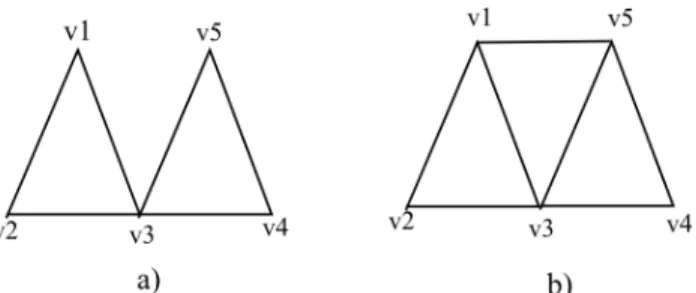
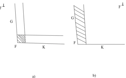
Figure 3.1. In Example 3.2.9, we consider two abstract simplicial complexes

a) and b). Both complexes include the 2-simplices shown; thus they are two dimensional. By Theorem 3.2.7, ∆1 in a) is not Cohen-Macaulay while ∆2 in b)

is.

Example 3.2.9. In Figure 3.1, there are two abstract simplicial complexes complexes of

(29)

for each simplicial complex and apply Theorem 3.2.7 to determine if each quotient is Cohen-Macaulay. In Fig. 3.1a), I∆1 = x1x5, x1x4, x2x4, x2x5¡and dim R/I∆1 = 3. From the figure,

one can see that the link of v3 consists of two disjoint one-dimensional faces. Thus H0(Lk(v3))

0 and R/I∆1 is not Cohen-Macaulay. By contrast Fig. 3.1b), I∆2 = x1x4, x2x4, x2x5 ¡, but

again dim R/I∆2 = 3. The edges have vertices as links, so their links vacuously satisfy the

Reisner criterion. The vertices have as their links a simply-connected union of edges, so their links satisfy the criterion also. Therefore, R/I∆2 is Cohen-Macaulay.

3.3. Radical Monomial Ideals in General Conical Algebras

If we replace the positive orthant by a more general positive rational cone C lying in Rd, there are natural generalizations of the radical monomial ideals. We will let I∆ be the ideal

generated by monomials that lie off a given subcomplex ∆ of faces of C.

Miller [17] derives a condition that k[C]/I∆ is Cohen-Macaulay using the Zeeman double

complex. He shows that the Zeeman double complex is an irreducible resolution for k [C]-modules and then shows that one of the spectral sequences arising from this double complex gives a minimal irreducible resolution when k[C]/I∆ is Cohen-Macaulay.

Cohen-Macaulay Complexes

First, we generalize the notion of ∆ being Cohen-Macaulay.

Definition 3.3.1. Let ∆G = {FP ∆| F G}.

We now define C(∆G), the algebraic cochain complex on the faces of ∆G. Let be an incidence function onLC. (See Definition 3.5.3.) For F P∆, letkF be a one dimensional vector space indexed by F. We denote the basis vector of kF by eF. So

C(∆G) = 0. . . C0 Ñ . . . Cd1 . . . CdÑ 0 Ñ. . . where

Ci ₌ à

FP∆G

dim F = i

(30)

Let dim F =`. The differential is defined

(3.4) B`peFq

¸

KP∆G

dim K =`+ 1

pK, FqeK.

Note that ∆G is not a subcomplex, since ∆G consists of only those faces which contain G.

Definition3.3.2. The modules HG(∆) = H(∆G) are called thelocal cohomology modules of ∆ near G.

Remark 3.3.3. Miller states that C(∆G) is isomorphic to the shifted reduced cochain complex ˜C(link∆(G)) of the “link of G in ∆” without specifically defining the link for a

polyhedral complex.

Definition 3.3.4. The polyhedral complex ∆ is a Cohen-Macaulay complex if the local

cohomology near every face G P∆ satisfies H_Gi(∆) = 0 for i dim ∆.

To verify that R/I∆ is Cohen-Macaulay, Miller constructs a double complex that is an

irreducible resolution for R/I∆, using an idea of Danilov [5].

Irreducible Resolutions and the Zeeman Double Complex

Definition 3.3.5. An ideal I is irreducible if I cannot be expressed as the intersection of

two ideals properly containing it.

Definition 3.3.6. An irreducible resolution of a k[C]-module M is an exact sequence 0 Ñ M Ñ W0 Ñ W1 Ñ. . . where Wn =

µn

à

j1

k[C]/Inj

such that each Iij is an irreducible ideal. Here the µi are the number of terms in each direct

(31)

For a face F of C, let kF be the 1-dimensional vector space spanned by F. For each face FP∆, letk[F] be the conical algebra for F, viewed as a quotient of k[C] and denote eF as the generator ofk[F]. Consider thek[C]-module D(∆) = à

FG

kFbk[G] generated by

{Fb eG |F, GP∆ and FG},

with k[C] acting on the second factor. The Zeeman double complex D(∆) is then defined so that D(∆)pq is generated overk by

{FbeG |p = dim F and -q = dim G}. Define the vertical differential B and the horizontal differential δ as

(3.5) B(eG) =

¸

dim G = dim G1+ 1

(G,G1)eG1

and

(3.6) δ(F) = ¸

dim F1= dim F + 1

(-1)q(F1,F)F1,

whereis an incidence function on ∆. This gives us the diagram:

Fb BeG

FbeG ÝÝÝÝÑ δF beG .

Recall the total complex of D(∆), totD(∆), is the complex whose ith term is à p qi

D(∆)pq with differential B + (-1)qδ. The importance of this double complex is given by the following result.

Theorem 3.3.7 (Theorem 3.4 of [17]). The total complex totD(∆) of the Zeeman double

complex D(∆) is an irreducible resolution of R.

(32)

Cohen-Macaulay, then the E2-term of the spectral sequence for the horizontal filtration gives a minimal resolution. Also, the spectral sequence obtained from the vertical filtration always converges at E1.

Definition 3.3.8. The Zn-graded Zeeman spectral sequence is the spectral sequence ZEpq

arising from the natural horizontal filtration of D(∆).

The following theorem (Theorem 4.2 of [17]) gives a characterization of the Cohen-Macaulay property in terms of irreducible resolutions coming from D(∆).

Theorem 3.3.9 (Miller). The following statements are equivalent.

1.R/I∆ is Cohen-Macaulay.

2. The complex ZE1 is a minimal linear irreducible resolution for R/I∆.

3. ∆is a Cohen-Macaulay complex.

3.4. Non-Radical Monomial Ideals in Polynomial Rings

We return to the case of a polynomial ring but now consider ideals which are not necessarily radical. Bayer, Peeva, and Sturmfels [1] identify a class of non-radical ideals which they call

generic ideals. For these ideals, they construct a minimal free resolution called the Scarf resolution. Using an associated simplicial complex called the Scarf complex, they are able to compute the depth.

The Taylor Complex and Taylor Resolution

Again, C is the positive orthant in Rd. So R =k[C] = k[x1,x2,. . . ,xd], the polynomial ring in d variables. Let {xm1_,xm2_{,. . .,x}mn_} _{be a minimal set of monomials generating I} _{R. For}

each subset S {1,. . .,n}, let xmS _{= lcm}

sPS {x

ms_}_{. Define} _m

(33)

is the module à St1,...,nu

R(-mS) with basis {eS} for S {1,. . .,n} with differential

(3.7) d(eS) = ¸

sPS

(-1)s 1 x

mS

xmSzs eSzs.

So the Taylor resolution of R/I can be written as

0Ñ à

dimSn1

R(-mS) Ñ à

dimS1n2

R(-mS1)Ñ. . .ÑRÑR/IÑ0.

Additionally, given the standard (n-1)-simplex, we may define a labeled simplicial complex ∆ and a corresponding chain complexF∆such thatF∆is the Taylor resolution. Let the vertices

vi of ∆ be labeled by mi, a minimal generator of I. Label each face F = {vi1,. . ., vis} of ∆ by

mF, where xmF = lcm v_ijPF {x

m_ij_}

. The exponent vectors of the monomials define a Zd-grading on the chain complex F∆ of ∆ over k[C]. We obtain this chain complex by making the usual

differential d homogeneous. For instance, let the label of v1 = x2y3 and the label of v2 = xz4.

Consider the edge e12. Then d(e12) = z4e1 - xy3e2. We say that the labeled simplex ∆ is the

Taylor complex.

Theorem 3.4.1 (Taylor [24]). The Taylor resolution is a free resolution for R/I.

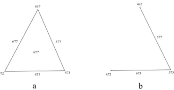
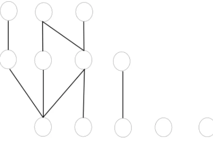
Figure 3.2. For the generic ideal I = x4y6z7,x5y7z3,x6y7z2 ¡ in Example

3.4.2, a) is the Taylor complex of I and b) is the Scarf complex of I. The label for a face F is expressed as abc, where xm_F = xaybzc.

Example 3.4.2. Let I = x4y6z7,x5y7z3,x6y7z2 ¡. The associated Taylor complex is

(34)

of I is formed. Note if a face F of the Taylor complex is deleted to form the Scarf complex, then every face G containing F is also deleted.

The Scarf Complex and Scarf Resolution

The Taylor resolution is far from minimal, because in general there will be distinct subsets K, L of {1, . . .,n} which have the same label. In other words, the Taylor complex will have faces with the same least common multiple. We know that any free resolution is a direct sum of the minimal resolution with trivial algebraic complexes. To obtain this minimal resolution, Bayer, Peeva, and Sturmfels introduce the following genericity condition.

Definition3.4.3. I is agenericmonomial ideal if I = xm1_,xm2_{,. . .,x}mn¡_{and no variable}

has the same nonzero exponent for any two minimal generators.

To identify the terms of the minimal resolution, we will consider the Scarf Complex of I: ∆I :={K{1,. . .,n}|mK mJ for any J {1,. . .,n}, J K}.

Note that the Scarf complex defines a subcomplex of the Taylor complex. See Example 3.4.2 and Figure 3.2b. We call the resolutionF∆I, defined by the Scarf Complex ∆I,the Scarf

resolution of R/I. The importance of the Scarf complex and the induced resolution is given in the following theorem.

Theorem 3.4.4 (Bayer, Peeva, Sturmfels [1]). If I is generic, then F∆I is a minimal free

resolution of R/I.

(35)

Computing the Depth of R/I using the Scarf Complex

We enlarge the set of generators of I to include monomials, xD_i ,1 ¤ i ¤ d, for sufficiently large D, to form a new ideal I, which has n + d generators. For every facet F of ∆I, there is a corresponding irreducible ideal

IF = xsii |D¡ si = degxi (mF)¡.

By the following theorem, one can construct the irreducible decomposition of I.

Theorem 3.4.5. A generic ideal I is the intersection of the irreducible ideals IF, where F

ranges through all facets of ∆I. This intersection is minimal.

One can now calculate the depth of I by using this minimal irreducible decomposition. By the Auslander-Buchsbaum formula, the depth(R/I) = depth(R) - pd R/I. depth(R) =

k[x1,x2,. . . ,xd] is d. The projective dimension of R/I is the maximum of the dimensions of the facets of ∆I, which, in general, is not a pure complex. However, every facet of ∆I extends to a facet of ∆I, which is pure of dim d-1. Conversely every facet of ∆I contains a face of ∆I. Thus, determining whether R/I is Cohen-Macaulay is equivalent to determining the dimensions of these irreducible components. Note

dimpIFq dimpR{IFq

d - the number of variables of xmF _{whose exponents are less than D.}

|F X tn 1, . . . , n du |, since F is pure of dim d-1 (3.8)

The following theorem is Corollary 3.9 of [1].

Theorem 3.4.6 (Bayer,Peeva, Sturmfels). Let I be a generic ideal of R = k[x1,x2,. . . ,xd].

Let I be minimally generated by n monomials. Then

depth (R/I) = min facets F of∆I

(36)

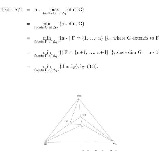
Proof. We have the following string of equalities.

depth R/I n max

facets G of ∆I

tdim Gu

min

facets G of ∆I

{n - dim G}

min

facets F of ∆I

tn -|F X{1,. . ., n} |u,, where G extends to F

min

facets F of ∆I

t|FX{n+1,. . ., n+d} |u, since dim G = n - 1

min

facets F of ∆I

tdim IFu,by (3.8).

l

Figure 3.3. ∆Ifor the ideal I = xy2z3, x3yz2, x2y3z¡ in Example 3.4.7. Here, only the vertices are labeled.

Example 3.4.7. Let I = xy2z3, x3yz2, x2y3z¡, which is generic. Then ∆I is the triangle

with vertices labeled {123},{312}, and {231}. Enlarging I to I, we see that ∆I shown in Figure 3.3 is the triangulation of the 2-simplex. Since the 2-simplex F in the center does not have a vertex on any coordinate axis, dim IF = 0. So depth (R/I) = 0.

3.5. Computing Local Cohomology using the L-complex

(37)

the local cohomology for R a conical algebra. The main advantage of this complex is that it will beZd-graded.

Computing Local Cohomology using the modified Cˇech Complex

We first introduce a complex whose cohomology gives us H_m(M). Let (R,m) be a Noetherian local ring with x1,x2,. . . ,xn be a system of parameters. Let Rxi₁xi₂...x_ij denote the localization

of R with respect to the multiplicatively closed set {(xn1

i1x

n2

i2 x

nj

ij), ni ¥0 for all i}. Define

themodified Cˇech complex:

C: 0Ñ C0 Ñ C1 Ñ. . . Cn Ñ0, where C`= à

1¤i1 i2 ...i`¤n

Rxi₁xi₂...x_i` and C

0 _{= R.}

The component of the differential d`: C` Ñ C` 1 mapping to Rxj₁xj₂...x_j`x_j` ₁

d`_|_R

xk_ixk₂...xk_`: Rxkixk2...xk` Ñ Rxj₁xj₂...x_j`x_j` ₁

is defined by

= $ ' ' ' ' ' & ' ' ' ' ' %

p1qs1iprq, iftk1, k2, . . . , k`u tj1, j2, . . . ,jˆs, . . . , j` 1u

0, otherwise

,

wherei is the inclusion map.

The following theorem allows one to compute the local cohomology using the above complex.

Theorem 3.5.1 ([2], Theorem 3.5.6). Let M be an R-module. Then

H_mi(M) Hi(M b C) for i¥ 0.

L-Complex

We now introduce the L-complex which generalizes the ˇCech complex to the case of a conical algebra. This complex is due to a similar one constructed by Goto and Watanabe [22]. A more thorough discussion is found in Section 6.2 of [2].

(38)

conical algebra. Recall from Section 3.1, that the monomials which lie in a face F make up a multiplicatively closed set S. For any face F of C, we let k[C]F = S1k[C], the localization of k[C] by S. Furthermore, there is a naturalZd-grading on k[C]. We show that k[C]F is also graded.

Proposition3.5.2. RF, when viewed as the k-vector space, has as a basis{xm |(m,ai)¥0

for all Hi PHF}.

Proof. RF = {x

c

xv, c P C, v P F} modulo the equivalence relation for localization. Let

xc

xv P RF and letm=c - v. Suppose there exits c1 PC andv1 in F such thatm= c- v = c1 - v1. Then xm = _xxvc = x

c1

xv1. So we have

xcxv1xc1xv xc v1 xc1 v

xpm+vq v1xpm v1q v

0.

Therefore, _xxvc = x c1

xv1 in RF. So there is a well-defined correspondence between elements

xc

xv of

RF and xm, where m=c - v.

Let m= c - v where c P C and v PF. Then (m,ai) = (c - v,ai) = (c,ai)¥ 0 for all Hi P

H_F. Conversely, if (m,ai)¥0 for all Hi PHF then there exists avPF such that (m+v,ai)¥ 0 for all Hi PH. Thereforem+ v=c PC. Thus m=c - v.

Suppose¸bi x

ci

xv_i 0 in RF, bi Pk. Without loss of generality, we can assume thatci - vi are distinct. Letv1_i = ¸

ji

vj. Let ˆv =°vi. Letc1_i =ci +v1_i. Note that thec1_i are also distinct. Multiplying each term in the sum by xv1

xv1 gives

¸

bi xci v 1

i

xˆv =

¸ bi xc

1

i

xˆv 0.

Therefore there exists a v1 PF such that xv1( n ¸

i1

bi xc1i) = 0. Since C is_Zd-graded, this implies

(39)

Therefore, for any face F of C and any m, we have dimk(RF)m ¤1. By the above lemma

RF k[x1,x₁1,. . .,xd,xd1]. Thus RF inherits a Zd-grading. Since IRF has an induced multi-grading from RF, the quotient RF/IRF has an induced Zd-grading.

Definition of the L-complex

The following facts are taken from [11].

Definition 3.5.3. Let LC be the face lattice of the cone C. Then : LC LC Ñ {0,1}

is an incidence function onL_C if satisfies the following: 1)(F,G) 0 if and only if G is a face of F;

2)(v,{0}) = 1 for all 1-dimensional faces v;

3)if e is a 2-dimensional face, and v1 and v2 are its one-dimensional subfaces, then

(e,v1) + (e,v2) = 0;

4)if F is an i-dimensional face and K is an (i + 2)-dimensional face with F K, then

(K,G1)(G1,F)+(K,G2)(G2,F)=0

where G1 and G2 are the unique (i+1)-dimensional faces that are both faces of K and contain

F.

We can now define the L-complex associated with R =k[C] (See [2],Chapter 6.2):

L : 0 ÑL0 Ñ L1 Ñ L2 Ñ. . .Ñ Ld Ñ0, where Li = à

dim Fi RF.

We note that L0 = R_p0q= R. To define the differentials, let F be a face of C such that dim F =

i. It suffices to define each restriction map B_|RF: RF Ñ

à

dim G = i + 1

RG. For r PRF, we define B|RF(r) =

¸

dim G = i + 1 FG

(G,F)iF,G(r),

where iF,G: RF Ñ RG is the natural inclusion map.

(40)

is mapped toxm. Thus the differential preserves the grading and we consider the m-graded local cohomology modules (L)m.

Example 3.5.4. Consider the positive orthant in Rd as a cone. Recall that for the ˇCech complex, the components of Cn are of the form Rxi₁...xin. We can view these localizations as

RF, where F is the face of the n-simplex spanned by eii,. . .,ein, and0. Thus, the L complex

is a generalization of C.

The following theorem states that the L-complex provides an alternate way to compute the local cohomology.

Theorem 3.5.5 (([2], Theorem 6.2.5). Let C be a positive rational cone. For every k

[C]-module M and for all i¥ 0, we have H_mi(M) Hi(Lb M).

By Theorem 3.5.5, we can use the L complex to compute the local cohomology of M = R/I, where R is a conical algebra corresponding to a rational positive cone C and I is a monomial ideal. Then, Lj b R/I = à

dim Fj

RF/IRF. The differential is B b id|R{I, and is defined by projection

B|RF{IRF(r) =

¸

dim G = dim F + 1 FG

(G,F) iF,G(r),

where iF,G:RF/IRF Ñ RG/IRG is the inclusion map. By Proposition 3.5.2, RF/IRF has a multi-grading. Thus L bR R/I admits a Zd-grading, namely (L bR/I)m =

à

(RF/IRF)m

and the differential preserves the multi-grading. Thus, one can compute the local cohomology for every multi-degreem. We then use Theorem 2.4.3 to compute the depth.

In the next chapter, we show that we may compute H((LbR/I)m) in terms of the

(41)

CHAPTER 4

Monomial Ideals in General Conical Algebras

In this chapter, we shall develop a method for computing the graded local cohomology of a conical algebra of the form R/I, where R = k[C] and I is a monomial ideal at a multi-indexm, as the topological cohomology of a compact polyhedral pair (Sm,Bm) defined by m. We shall

call these ringsmonomial algebras. Furthermore, we decomposeRdintocritical regions so that for allmin a critical region, the pair (Sm,Bm) is constant. In section 1, we recall the theory of

polyhedral complexes, specifically the relative cochain complex of a polyhedral pair. In section 2, we establish the isomorphism between (LbR/I)mand the shifted relative polyhedral cochain

complex of (Sm, Bm). To identify the critical regions, we introduce in section 3 a collection

of projection maps and examine the image of C and I under these projections. In section 4, for each critical region, we compute the compact polyhedral pair associated to the region. In section 5, we determine the cohomology of this pair. This allows us to give bounds on the depth in terms of the topology of the polyhedral pairs for each of the critical regions. Using these bounds, we deduce necessary and sufficient conditions that k[C]/I is Cohen-Macaulay.

4.1. Polyhedral Complexes

In this section, we recall some definitions and results about polyhedral complexes. In the case of a rational cone C, we recall the definition of a transversal cross-section. Some of the definitions from Section 3.5 are repeated.

Definition 4.1.1. A convex polyhedron P is the intersection of a finite number of closed

(42)

Given H a hyperplane and aH a normal vector to H, we denote the positive half-space determined by aH by

H tv| pv, aHq ¥0u.

Then we may write P = r_i₁ H_i , where the normal vectors ai) = aHi point into P and the

H_i are distinct. We also note that this intersection of half-spaces may not be minimal. Below, we identify those hyperplanes which form a minimal representation of a convex polyhedron P.

Definition 4.1.2. Hj is a basic supporting hyperplane of a convex polyhedron P if £

ij

H_i P

Definition 4.1.3. Let P be a convex polyhedron. AfaceF of P is the intersection of P and

a collection of basic supporting hyperplanes {H_i} of P. We let F¡ denote the smallest affine

space containing F. The dimension of a face F is dim F¡. G is a subface of F if G is a face of P and G F.

Remark 4.1.4. For us, the first important example of a convex polyhedron is a rational

positive convex cone CRd, whereRd denotes all d-tuples whose coordinates are non-negative real numbers.

We will next consider a special class of subcomplexes of convex polyhedra.

Definition 4.1.5. A finite set of faces S of a convex polyhedron will be called a polyhedral

complexif:

1) the intersection of any two faces in S is either empty or a subface of each, and

2) if F P S and G F, then GP S.

If A is a polyhedral complex, and every face in A lies in S, A is a polyhedral subcomplex of S.

(43)

Definition4.1.6. Amaximal faceF of a polyhedral complex S is one which is not contained

in a larger face of S. Then, the polyhedral complex S is said to be pure if all the maximal faces of S have the same dimension.

Definition 4.1.7. Let S be a polyhedral complex. For a face F P S, we define the star

complex of Fto be StS(F) ={GPS |there exists KPS such that G, F K}. The boundary of the star complex of Fis defined as BStS(F) ={GPStS(F)|FG}. Also, the complementary complex of F is defined to be CplS(F) = {GP S |F G }.

We observe that StS(F), BStS(F), and CplS(F) are subcomplex of S, and that

CplS(F)YStS(F) = S and CplS(F)XStS(F) = BStS(F). In [9], the star complex is called the closed star of F, since it includes all subfaces of G F. The (open) star of F is defined as all faces strictly containing F.

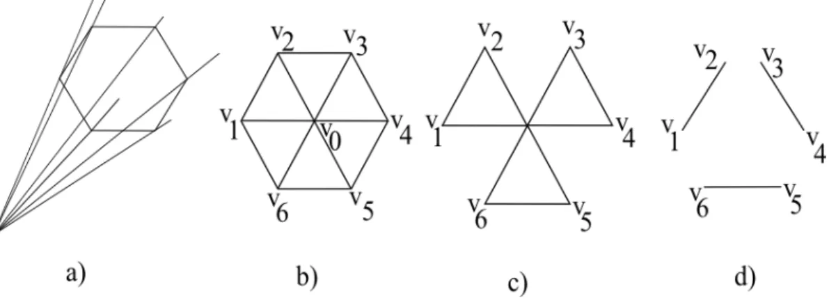
Figure 4.1. For the cone C in Example 4.1.8 given by a), we have a

represen-tation of its boundary faces in b). For the polyhedral subcomplex S given in c), BSt({v0}) is shown in d).

Example 4.1.8. Let C be a positive cone on a hexagon in R3 as in Figure 4.1 a). The faces of the cone form a polyhedral complex. We represent P in Fig 4.1 b) as a hexagon by labeling the vertices {v1,. . .,v6}. Then we create six triangles within the hexagon, all with a

common vertex v0. v0 represents the face {0}, while the triangles represent the maximal two

(44)

(Fig 4.1 d) is not equal to the topological boundary of StS(v0). We remark that in this case

BStS(v0) = CplS(v0).

We next give a basic topological property of the star complexes StS(F).

Lemma4.1.9. For a polyhedral complex S and any non-empty face F, StS(F) is contractible.

Proof. Let K1,. . .,Kr be maximal faces of StS(F). By definition, F r £

i1

Ki. Let x be a point on F. Let si: Ki [0,1] Ñ Ki be the straight-line homotopy given by

si(y,t) = (1-t)y + tx

Since each Ki is convex, the line segment lies entirely in Ki. If any two maximal faces Ki, Kj intersect in a face G, the line segment also lies in G because all faces are convex. Individually these are deformation retracts of each Ki ontox. Let r: StS(f) [0,1]Ñ StS(f) be

r(y,t) = si(y,t) when y PKi.

Since the si agree on any overlap, r is well-defined. Thus, r is a deformation retraction of StS(f)

onto {x}. l

Transversal Cross-Sections of Cones

Let C be a positive rational cone inRd as defined in Section 2.2. We consider a transversal hyperplane to C. This is a hyperplane T which is transverse to every positive ray in Rd. Such planes are defined by normal vectors whose coordinates are all positive. We shall call D = CXT atransverse cross-section of C. Note that if GF, then GXTFXT. Then we have a 1-to-1, order-preserving correspondence Θ between the faces of C and the faces of D, where Θ(F) = FXT. We shall denote the face of a cross-section corresponding to F by f. We include the empty face {H} as a face of D. So we set Θ({0}) = {H}. Note that the empty face {H}

(45)

Remark 4.1.10. We wish to distinguish the empty face {H} of a polyhedron from the

empty complexHconsisting of no faces. This distinction will be more evident when we discuss the cohomology of polyhedral complexes.

The following lemma relates the transversal cross-section for two different transverse hyper-planes.

Lemma4.1.11. i)Suppose T, T1 are transversal planes defining cross-sections of C with D =

T X C , and D1 = T1 X C. Then there exists a homeomorphism ψ:D Ñ D1 which preserves

the face decomposition.

ii) Let S be a polyhedral subcomplex of C. Then S = SXT is a polyhedral subcomplex of D. If

S1 = S XT1, then ψ restricts to a face-preserving homeomorphism S ÑS1.

Proof. i)If T2 is a plane through the origin parallel to T1, then the central projection

from 0 onto T1 π : Rdz T2 Ñ T1 is a smooth map. Let x P f D. Then there exists a ray R x FC such that R xXD = x. Then, by transversality of T1 to theR x, there exists a unique point yx PF1 X D1 = f1 such that yx = rx for some r PR . This defines a mapψ: DÑ D1 whereψ(x) = yx. ψ =π|D, soψ is smooth.

By the same process, there is a smooth map φ: D1 Ñ D mapping yx to x. Now φψ = idD andψφ= idD1. Furthermore, ψ(f) = f1.

ii)Let S be a polyhedral subcomplex of C. If F, F1 S and F XF1 = G, then g (possibly the empty face) is a subface of both f and f1. Also if G F, then G X T F X T. Thus S is a polyhedral subcomplex of D. Since ψ preserves the faces of S,ψ maps S homeomorphically

onto S1. l

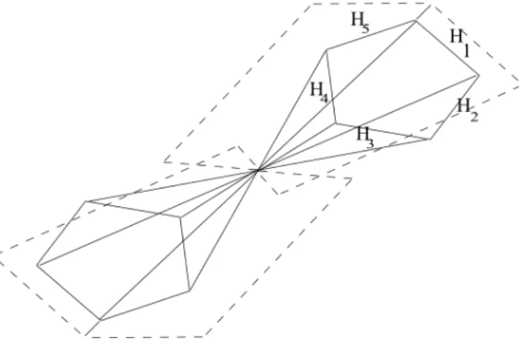
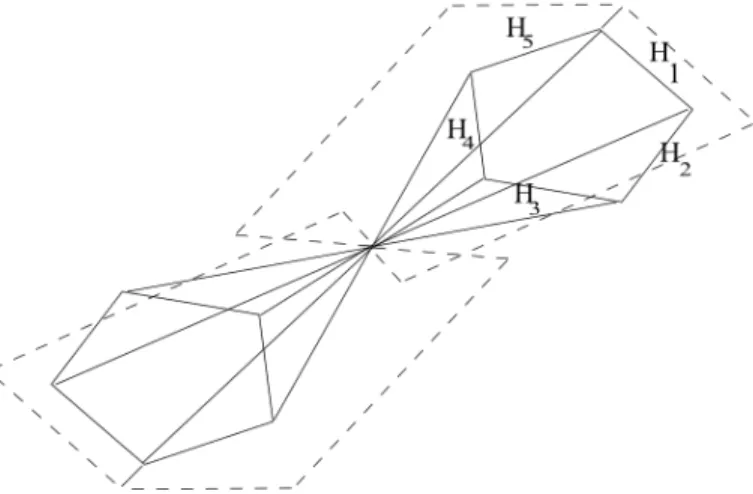
Example 4.1.12. In Figure 4.2, C is a three-dimensional cone with basic supporting

hy-perplane H1, . . . H5. The cross-section of C is a pentagon. In Figure 4.2, we also show -C =

(46)

Figure 4.2. A three dimensional cone C, with cross-section along with -C. The

basic supporting hyperplanes of C are labeled H1,. . .H5. See Example 4.1.12.

A cross-section D of C lies in the (d-1)-simplex TXRd and hence is bounded. A bounded polyhedron is called a polytope. As a topological space, a polytope is compact. Hence, any polyhedral subcomplex of any polytope is compact. We now connect the singular cohomology of a compact polyhedral pair to the cohomology of the cochain complex for compact polyhedral pairs.

4.2. Cochain Complexes for Polyhedral Complexes

In this section, we recall the cochain complex associated to a polyhedral complex. More specifically, we define the relative cohomology of a polyhedral pair. We will recall the fact that the polyhedral complexes are special cases of regular cell complexes to relate the (topological) cohomology of the polyhedral pair to the cohomology of the cochain complex determined by that pair.

LetLP be the face lattice of a polyhedral complex P, which is the set of faces of P ordered by inclusion. Letbe an incidence function onLP. (See Definition 3.5.3.) We may then restrict this to an incidence function for a polyhedral subcomplex SP.

Remark4.2.1. [Incidence Function on a Polytope] Given a polytope D, we may also define

(47)

2)(v,H) = 1 for all vertices v ,

3)if e is a 1-dimensional face, and v1 and v2 are its vertices, then

(e,v1) +(e,v2) = 0.

If there is an incidence functionon the face lattice of a cone C, theninduces an incidence function1on the face lattice of any transverse cross-section via the map Θ described in Section 4.1 by1(f,f1) =(F,F1).

Remark 4.2.2. The incidence function for polytopes is equivalent to putting a consistent

orientation on the faces of D in the following way, as described in Theorem 7.2 of Chapter IX of [11]. We use induction on the dimension of the faces. Given an edge e, there are two unique vertices that satisfy condition 4. Without loss of generality, suppose that v1 satisfies

(e,v1) = 1. Assign an arrow to e such that the arrow is pointing away from v2 and toward

v1. Thus we have an orientation on all edges. Suppose f has dimension k, and there exists an

orientation on all faces having dimension less than k. If (f,f1) = 1, then the orientations on f1 is the induced orientation from f when we view f as a piecewise linear manifold with boundary. If(f,f1) = -1, then f and f1 have opposite orientation, that is the induced orientation on f1 from f is the negative of the given orientation on f1. In this way one can construct on orientation on the k-dimensional faces of S by knowing the orientations of all 0,1,. . .,(k-1)-dimensional faces.

Using these incidence functions, we introduce chain and cochain complexes for polyhedral subcomplexes of both convex polyhedral cones and polytopes.

Chain Complexes for a Polyhedral Cone

Let S be a d-dimensional polyhedral subcomplex of a polyhedral cone, and let be an incidence function on LS. Define the (non-augmented) chain complex to be

(48)

where

(4.2) C`(S) =

à

FPS dim F =`

kF.

wherekF is the one-dimensionalk-vector space corresponding to the face F. We abuse notation and denote the generator by F, as well. The differential is given byB`: C`(S)ÑC`1(S), where

(4.3) B`(F) = ¸

F1FPS

dim F1=`-1

(F,F1)F1.

Property 3 of Definition 3.5.3 implies that B2 B1 = 0, while Property 4 implies that B`

B`1 = 0 for all`¡ 2.

Let A be a polyhedral subcomplex of S, with face sublatticeLALS. Then, for every i¥0,

Ci(A) = à

GPA dim G = i

kG is a vector subspace of Ci(S). Since A is a polyhedral subcomplex,|LA is

an incidence function onLA. ThusB sends Ci(A) to Ci1(A), andB induces a homomorphism

on the quotient space Ci(S,A) = Ci(S)/Ci(A). If A is the empty complex, then C(S,A) = C(S). These quotient spaces along with the differentials Bt form a chain complex called the

reduced chain complex of the pair (S,A):

(4.4) C(S,A): 0ÑCd(S,A)ÑCn1(S,A)Ñ . . .C0(S,A)Ñ 0.

Define Ci(S, A) = (Ci(S, A)) to be the dual vector space of Ci(S, A). Let F be the dual basis vector that is 1 on F and zero on the other faces. The set{F|F a face of S and dim F = i} form a basis of Ci(S). Likewise, the set {F | F a face of S, not a face of A and dim F = i} form a basis of Ci(S, A). The transpose of B, which we call δ, gives a mapδr: Cr(S, A) Ñ Cr 1(S, A) defined by

δr(F) = ¸ FF1PS

dim F1= r+1