eCognition Developer
Tutorial 4 ‐ analyzing areas of interest with regions & maps
Introduction 3 About this Tutorial 3 Requirements 3 Data included with the Tutorial 3 Lesson 1 – Introduction to the analysis workflow 4 Lesson 2 Classifying regions of interest via a map with lower resolution 5 2.0 Lesson content 5 2.1 Process se駫�ngs to create a map 5 2.1.1 Create and explore the new map 7 2.2 Classifying the map 8 2.3 Synchronizing the results to the main map 9 Lesson 3 Detailed analysis of water bodies 11 3.0 Lesson content 11 3.1 The overall looping process 12 3.2 Selec갇ng one object and crea갇ng the region and map 12 3.2.1 Selec갇ng the object 12 3.2.2 Crea갇ng a region and a map 14 3.3 Processing on ‘Map Detail’ and synchroniza갇on 16 3.3.1 Classifying ‘Map Detail’ 17 3.3.2 Synchronize the results back to main map 18 Lesson 4 The complete classification 20 4.0 Lesson content 20 4.1 Prepare the next looping sequence 20 4.2 Execute the complete sequence step by step 20 4.3 Execute the sequence with ‘looping’ on 21 Where to get additional help & information? 22 The eCogni갇on Community 22 The User Guide & Reference Book 22 eCogni갇on Training 22
Introduction
About this Tutorial
This tutorial gives you an introduc갇on on how to combine both the maps and regions concepts to classify areas of interest in a fast and efficient way. You should have gone through the tutorial ‘working with regions’ and ‘working with maps’ prior to this tutorial. This Module has four lessons: ● Lesson 1 Introduc갇on to the analysis workflow ● Lesson 2 Classifying regions of interest via a map with lower resolu갇on ● Lesson 3 Detail analysis of water bodies using a detail map ● Lesson 4 The complete classifica갇on Further informa갇on about eCogni갇on products is available on our website: www.eCogni갇on.comRequirements
To perform this Guided Tour, you will need: ● eCognition Developer installed on a computer● A computer mouse is highly recommended
All steps of this tutorial can be done using the eCognition Developer or the free‐trial version . This tutorial is designed for self‐study.
Data included with the Tutorial
Image data
We will be working with a QuickBird satellite image (*.갇f) comprised of two files in this tutorial:
● ‘02MAR02_mul갇_Subset_Maps_Regions.TIF’ contains the RGB and NIR data
● ‘02MAR02_pan_Subset_Maps_Regions.TIF’ contains the panchromatic data
Rule Sets
A Rule Sets is available represen갇ng the final state of Rule Set development. Whenever the tutorial refers to a Rule Set, it can be found in the tutorial folder.
Project
Lesson 1 – Introduction to the analysis workflow
This tutorial gives you an introduc갇on into combining both the maps and regions concepts to classify areas of interest in a fast and efficient way. The analysis in this example is a con갇nuing interplay between maps, their classifica갇on and the synchroniza갇on of results.
The general setup of the Analysis rou갇ne:
A map with lower resolution (1) is created. The water bodies are classified (2) roughly on that downsampled map. The results are synchronized (3) back to the main map.
One water body object is picked out (4). From this
object, a region is created and from this region a map is created (5) in the same resolution .
This detail map is classified (6). The map is
synchronized (7) back to the main map. The next (4) water body object is picked, the process starts all over again with crea갇ng region from this object.
Lesson 2 Classifying regions of interest via a map with lower resolution
2.0 Lesson content
● The process se駫�ngs to create a map ● Classifying the map ● Synchronizing the results In the first part of the Rule Set, a map with a lower scale is created and the water bodies are classified roughly in this map. The results are then synchronized back to the main map. The advantage of this approach is that through the down‐sampling the segmenta갇on and classifica갇on is faster then running the classifica갇on on the original scene. For very large areas it is possible that the number of created objects is so high that processing is cancelled (i.e. due to lack of memory). This can be avoided by using the approach explained in this tutorial. Figure 3: Schematic diagram showing the workflow to create a map, classify it and synchronize it back.2.1 Process settings to create a map
The Project to be loaded contains a set of mul갇spectral and panchroma갇c image layers from a subset of a Quickbird scene. 1. Start eCogniton Developer . 2. Switch to predefined view se駫�ng number 4 ‘ Develop rulesets ’ 3. In the main menu ‘File’ choose ‘Open Project’ or click on the ‘Open Project’ bu姫�on in the toolbar. 4. Open the project ‘ AnalyzingRegionsOfInterest.dpr ’ in the tutorial folderFigure 1: Process to create a map with lower resolution.
6. Double‐click on the first child process ‘ copy map to 'Map_6m_px' with scale 6m\pxl ’ to open it.
● In the Algorithm Parameters the name of the target map (map to be created) ‘ Map_6m_px ’ is defined.
● In the field ‘ Image Layers ’ the Layers ‘ nir ’ and ‘ pan ’ are selected to be part of the new, downscaled map.
● In the field ‘ Scale ’ the resolu갇on of the new map can be changed.
Figure 2: Process settings to create a downscaled ‘Map_6m_px’.
7. Click on the ‘ … ’ next to the ‘Scale’ field, to open the ‘ Select Scale ’ dialog box.
● ‘ Keep current scene scales ’ must be deselected.
● As ‘ Scale Mode ’, ‘ Units ’ is chosen. Other scale modes are : magnifica갇on, percent and pixel.
Figure 3: The ‘Select Scale’ dialog box with settings to create a 6 m/px map.
8. Click on the ‘Cancel’ bu姫�on to close the dialog box.
2.1.1 Create and explore the new map
1. Execute the process.
2. Open a second viewer , display in the new created map and select ‘Side by side view’. 3. Display the ‘pan layer in both views.
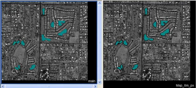
The newly created map contains only the panchromatic and near infrared image layers and has a lower resolu갇on of 6 m/px.
Figure 4: Main map in full resolution (left); new map with lower resolution 6 m/px (right).
2.2 Classifying the map
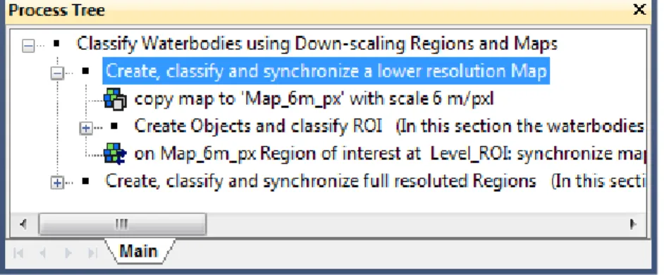
1. Expand the process sec갇on ‘Create Objects and classify ROI’.
● In parent process ‘ Create Objects and classify ROI ’ it is specified, that all subsequent child processes are applied only to ‘ Map_6m_px ’.
● A quadtree segmentation is executed.
● All objects with a mean value ≤ 210 in the panchroma갇c layer are classified as ‘Region of interest’ (ROI). ● Those ‘Region of interest’ objects with a mean ‘nir’ value ≥ 160 are declassified again. ● The ‘Region of interest’ objects are merged ● The ‘Region of interest’ objects with an area ≤ 30 pixel are de‐classified ● All unclassified objects are merged . ● All ‘Region of interest’ objects are grown by two pixels . Figure 5:Process Tree with process sequence highlighted to classify the ‘Map_6m_px’. 2. Execute the process sequence ‘ Create Objects and classify ROI ’. All water bodies are classified as ‘Region of interest’, a buffer of two pixels is added to every object. Figure 6: Classification before (left) and after (right) executing the growing process .
2.3 Synchronizing the results to the main map
The next step is to copy the classifica갇on results from ‘ Map_6m_px ’ to the main map. This classifica갇on will then become the basis for the crea갇on of the regions and maps for a more detailed analysis. 1. Collapse the process sec갇on ‘ Create Objects and classify ROI ’. 2. Double‐click on the first child process on ‘ Map_6m_px Region of interest at Level_ROI: synchronize map 'main' ’ to open it. ● In the Image Object Domain it is specified, that only the ‘Region of interest’ objects of ‘Map_6m_px’ are copied. ● In the Algorithm Parameters it is specified that the new created Level in the main map is named ‘Level_ROI’, same as in the map with lower resolu갇on. Figure 7: Process settings to synchronize the content of the ‘Map_6m_px’ to the main map. 3. Execute the process. The main map contains now a ‘Level_ROI’ with the ‘Region of interest’ objects.
Figure 8: Main map with synchronized content of the ‘Map_6m_px’ (left); content of ‘Map_6m_px’ (right).
Lesson 3 Detailed analysis of water bodies
3.0 Lesson content
● The overall looping processes
● Picking out an object and crea갇ng a region and a map
● Processing on ‘Map Detail’ and synchroniza갇on
In this sec갇on, the ‘region of interest’ objects are selected one a耀er the other. A region is created from the selected object and a new map with full resolu갇on is created from the region. A detailed segmentation and classification is then applied only to the detailed map. In addi갇on, objects are reshaped to ensure smooth
outlines. In a final step, the detail map is copied back to the main map and the procedure continues with the next object un갇l all are analyzed in detail. Figure 9: Schematic diagram showing the workflow to select an object and create a region and a map from it. Figure 10: Schematic diagram showing the classification of the new map and the synchronization.
3.1 The overall looping process
1. Collapse ‘Create, classify and synchronize a lower resolu갇on map’ and expand ‘ Create, classify and synchronize full resolution Regions ’.
2. Double‐click on the first child process on ‘ loop: while No. of Region of interest > 0 ’ to open it.
● In the Domain of the parent process, a Condi갇on is set. The feature used is a Class‐Related Scene feature ‘Number of classified objects’. The condi갇on is that the Number of ‘Region of interest’ objects must be more than 0 . This means at least one has to exist, otherwise the process (and all child processes) are not executed.
● The ‘Loops and Cycles’ is set to ‘ Loop while something changes only ’. As long as the Threshold condi갇on is fulfilled , the process will be re‐executed. Only if all ‘region of interest’ objects are classified as ‘Water’ the processing stops automa갇cally. Figure 11: Process settings to execute the child processes, as long as the Condition is fulfilled. 3. Close the ‘Edit Process’ dialog box by pressing the ‘Cancel’ bu姫�on.
3.2 Selecting one object and creating the region and map
In this rou갇ne, one object is selected (the one with the minimum in X), a region is created around this object and a detailed map is created from this region. 3.2.1 Selecting the object The objects are selected randomly, the object with the minimum value for X is classified to a class ‘_ac갇ve’. It is also possible to use other features, e.g. standard devia갇on or size. But it is important that the process is not classifying two objects at once to the ‘_ac갇ve’ class. 1. Expand ‘ loop: while No. of Region of interest > 0’ and expand ‘Pick out one 'Region of interest' Object ’.Figure 12: Process Tree with process sequence highlighted to select one ‘Regions of interest’ object, create a region from it and to create a map from this region. In the parent process ‘Pick out one 'Region of interest' object’ the main map is specified as domain. All child processes refer to this se駫�ng. 2. Double‐click on the first child process on ‘ Region of interest at Level_ROI: min X Center in domain : _active ’ to open it.
● The algorithm ‘ find domain extrema ’ is used to select an object.
● In the Domain, it is defined that only the ‘Region of interest’ objects are analyzed with the algorithm.
● The ‘ Extrema Type ’ is set to Minimum.
● As feature ‘ X Center ’ is chosen.
● The field ‘ Accept equal extrema ’ is set to ‘No’.
● The field ‘ Active class ’ is set to ‘_ac갇ve’. The object with the minimum X‐center will be classified to this class.
Figure 13: Process settings to classify an ‘_active’ object.
Figure 14: Main map with one ‘_active’ object classified.
3.2.2 Creating a region and a map
The last two processes of the sequence ‘Pick out one 'Region of interest' object’ create a region from the ‘_ac갇ve’ object and from the region a map.
1. Double‐click on the second child process on ‘ _active at Level_ROI: _active region= object region ’ to open it.
● The Domain is set to ‘ image object level ’. It is defined that the source for the region extent is class ‘_ac갇ve’ in the ‘Level_ROI’.
● The name of the new region is defined as ‘ _active region ’.
Figure 15: Process settings to create a region ‘_active region’ from the current ‘_active’ object.
2. Execute the process.
3. Double‐click on the next process on copy map to ' Map Detail ' to open it.
● In the field ‘ Source Region ’ it is defined that the ‘ _active Region ’, created with the process before, is the basis for the map extent.
● All other parameters are set as default , all image layers are copied in the new map and also the image objects with classifica갇on.
5. Display ‘Map Detail’ in the viewer. From the ‘_Ac갇ve Region’ in the main map a new map ‘Map Detail’ is created, containing the objects and classifica갇on from the main map. Figure 17: Main map with ‘_active’ object classified; newly created ‘Map Detail’ (inset).
3.3 Processing on ‘Map Detail’ and synchronization
In the sequence ‘ Process on Map Detail and synchronize ’ the classifica갇on of the ‘Map Detail’ is defined, as well as the synchroniza갇on back to the main map.
A耀er this sequence is executed, the remaining ‘_ac갇ve’ objects in the main map are declassified and the processing starts again with selec갇ng the next 'region of interest' in the main map.
3.3.1 Classifying ‘Map Detail’
In this sec갇on, the content of the water body in the current ‘Map Detail’ is classified. 1. Collapse ‘Pick out one 'Region of interest' object’.
2. Expand ‘Process on Map Detail and synchronize’ and expand ‘Classify Map Detail’. The process sequence ‘ Classify Map Detail ’ has 5 sec갇ons:
● The map is split up to pixel‐sized objects using the chessboard segmentation .
● In the sec갇on ‘ Find Seeds ’, first ‘Water’ objects are classified by measuring and classifying the darkest values for the panchroma갇c layer.
● In the sec갇on ‘ Grow ’, the first ‘Water’ objects are grown into spectrally similar neighbors.
● In the sec갇on ‘ Clean up ’, holes are filled and small ‘Water’ objects are declassified.
● In the sec갇on ‘ Object reshaping ’ growing and shrinking processes are applied to get smooth outlines for the ‘Water’ object Figure 19: Process Tree with process sequence highlighted to classify the current ‘Map Detail’. 1. Execute ‘ Classify Map Detail ’. Figure 20: ‘Map Detail’ before and after classification.
The last process in the ‘Process on Map Detail and synchronize’ sec갇on of the Rule Set is the synchroniza갇on of the ‘Map Detail’ with the main map.
1. Collapse ‘Classify Map Detail’.
2. Double‐click on the process ‘ Water at Level_ROI: synchronize map 'main' ' to open it.
● In the Domain it is specified, that the ‘Water’ objects are the objects to be synchronized. ● In the Algorithm Parameters it is specified, that main map is the target of synchroniza갇on and the objects shall be synchronized in ‘Level_ROI’. Figure 21: Process settings to synchronize the ‘Map Detail’ with the main map. 3. Execute the process. 4. Open a second viewer and display in one viewer the ‘Detail Map’ in the other the main map. Zoom to the synchronized ‘Water’ object. The classifica갇on of the ‘Water’ object in the ‘Map Detail’ has been copied in the main map.
Figure 22: The ‘Water’ object is synchronized in the main map (left); ‘Map Detail’ with ‘Water’ classified (right).
Lesson 4 The complete classification
4.0 Lesson content
● Prepare the next looping sequence ● Execute the complete sequence step by step ● Execute the sequence with ‘looping’ on4.1 Prepare the next looping sequence
To have everything cleaned up, the exis갇ng ‘_ac갇ve’ objects have to be declassified. Then the next ‘Region of interest’ object can be classified as ‘_ac갇ve’ and analyzed in detail. 1. Collapse ‘Process on Map Detail and synchronize’.2. Select ‘ on main _active at Level_ROI: unclassified ’ and execute the process. The remaining ‘_ac갇ve’ objects are de‐classified.
Figure 23: Before (left) and after (right) executing the declassification of the remaining ‘_active’ objects.
4.2 Execute the complete sequence step by step
1. Double‐click on the process ‘ loop: while No. of Region of interest > 0 'main' ' to open it. 2. In the field ‘Number of cycles’ insert 1.
3. Confirm the change with ‘OK’ bu姫�on.
4. Execute the sequence ‘ if No. of Region of interest > 0 ’ several 갇mes.
A耀er each execu갇on another ‘Map Detail’ is classified and another ‘Water’ object is synchronized in the main map.
Figure 24: Stepwise one ‘Region of interest’ object after the other is classified.
4.3 Execute the sequence with ‘looping’ on
1. Double‐click on the process ‘ if No. of Region of interest > 0 ' to open it. 2. In the field ‘Number of cycles’ choose ‘ Loop while something is changing ’. 3. Confirm the change with ‘ OK ’ bu姫�on.
4. Execute the sequence ‘l oop: while No. of Region of interest > 0 'main' '.
All ‘Region of interest’ objects are analyzed in a ‘Detail Map’ and synchronized back in the main map.
Figure 25: Classification of the main map after executing the complete sequence with ‘looping’.