Multi-scale Jump and Volatility Analysis for
High-Frequency Financial Data
∗
Jianqing Fan and Yazhen Wang
Version of May 2007
Abstract
The wide availability of high-frequency data for many financial instruments stimulates an upsurge interest in statistical research on the estimation of volatil-ity. Jump-diffusion processes observed with market microstructure noise are frequently used to model high-frequency financial data. Yet, existing methods are developed for either noisy data from a continuous diffusion price model or data from a jump-diffusion price model without noise. We propose methods to cope with both jumps in the price and market microstructure noise in the observed data. They allow us to estimate both integrated volatility and jump variation from the data sampled from jump-diffusion price processes, contam-inated with the market microstructure noise. Our approach is to first remove Jianqing Fan is Frederick Moore’18 Professor of Finance, Department of Operation Research and Financial Engineering, Princeton University, Princeton, NJ 08544. Yazhen Wang is professor, Department of Statistics, University of Connecticut, Storrs, CT 06269. Fan’s research was partially supported by supported by the NSF grant DMS-0532370 and Wang’s research was partially sup-ported by the NSF grant DMS-0504323. The authors thank the editor, associate editor, and two anonymous referees for stimulating comments and suggestions, which led to significant improvements in both substance and the presentation of the paper.
jumps from the data and then apply noise-resistant methods to estimate the integrated volatility. The asymptotic analysis and the simulation study reveal that the proposed wavelet methods can successfully remove the jumps in the price processes and the integrated volatility can be estimated as accurately as in the case with no presence of jumps in the price processes. In addition, they have outstanding statistical efficiency. The methods are illustrated by applications to two high-frequency exchange rate data sets.
1
Introduction
Diffusion based stochastic models are often employed to describe complex dynamic systems where it is essential to incorporate internally or externally originating ran-dom fluctuations in the system. They have been widely applied to problems in fields such as biology, engineering, finance, physics, and psychology (Kloeden and Platen, 1999, chapter 7). As a result, there has been a great demand in developing statistical inferences for diffusion models (Prakasa Rao, 1999). This paper investigates non-parametric estimation for noisy data from a jump-diffusion model. The problem is motivated from modeling and analysis of high-frequency financial data.
In financial time series there are extensive and vibrant research on modeling and forecasting volatility of returns such as parametric models like GARCH and stochastic volatility models (Bollerslev, Chou and Kroner, 1992; Gouri´eroux, 1997; Shephard, 1996; Wang, 2002), or implied volatilities from option prices in conjunction with specific option pricing models such as the Black-Scholes model (Fouque, Papanicolaou, and Sircar, 2000). These studies are for low-frequency financial data, at daily or longer time horizons. Over past decade there has been a radical improvement in
the availability of intraday financial data, which are referred to as high-frequency financial data (Dacorogna, Ge¸cay, M¨uller, Pictet and Olsen, 2001). Nowadays, thanks to technological innovations, high-frequency financial data are available for a host of different financial instruments on markets of all locations and at scales like individual bids to buy and sell, and the full distribution of such bids.
Historically the availability of financial data at increasingly high frequency allow us to incorporate more data in volatility modeling and to improve forecasting perfor-mance. However, because of their complex structures, it is very hard to find appro-priate parametric models for high-frequency data. Volatility models at the daily level cannot readily accommodate high-frequency data, and parametric models specified directly for intradaily data generally fail to capture interdaily volatility movements (Andersen, Bollerslev, Diebold and Labys, 2003).
It is natural to use flexible nonparametric approach for high-frequency volatility analysis. One popular nonparametric method is the so-called realized volatility (RV) constructed from the summation of high-frequency intradaily squared returns (An-dersen, Bollerslev, Diebold and Labys, 2003; Barndorff-Nielsen and Shephard, 2002), and another one is the realized bi-power variation (RBPV) constructed from the sum-mation of appropriately scaled cross-products of adjacent high-frequency absolute returns (Barndorff-Nielsen and Shephard, 2006). Theoretical justifications of these nonparametric methods are based on the idealized assumption that observed high-frequency data are true underlying asset returns. Under this assumption, asymptotic theory for RV and RBPV is established by connecting them to quadratic variation and bi-power variation. RV and RBPV are combined together to test for jumps in prices and to estimate integrated volatility and jump variation.
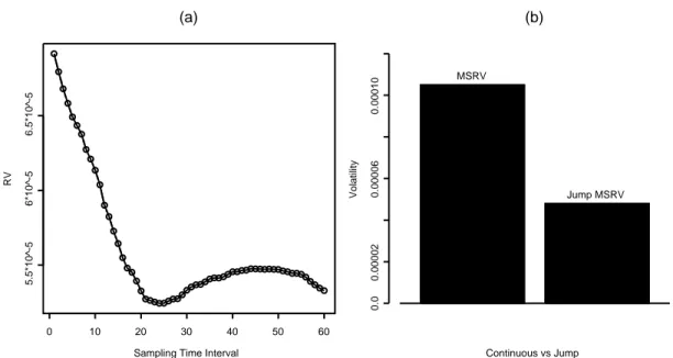
Sampling Time Interval RV 0 10 20 30 40 50 60 5.5*10^-5 6*10^-5 6.5*10^-5 (a) 0.0 0.00002 0.00006 0.00010 Continuous vs Jump Volatility MSRV Jump MSRV (b)
Figure 1: (a). Plot of the RV as a function of sampling time interval in minute. The
horizon axis is the time interval in minute that the data are sampled from Euro-dollar exchange rates on January 7, 2004, for computing the RV. The shorter the sampling time interval is, the higher the sampling frequency. The RV shoots up as the sampling time interval gets shorter, which suggests the presence of the microstructure noise. (b). Plot of estimated integrated volatility using MSRV for Euro-dollar exchange rates on January 9, 2004. The bar on the left panel shows the estimate of integrated volatility obtained by applying MSRV to the whole data, and the right panel indicates the sum of the four estimated values obtained by applying the same MSRV procedure to each of the four pieces of the data. The left panel estimate is twice as large as the estimate in the right panel, which indicates the existence of jumps.
The idealized assumption is, however, severely challenged by high-frequency data. In reality, high-frequency returns are very noisy and hence do not allow for reliable inferences of RV and RBPV regarding the true underlying latent volatility. The noise is due to the imperfections of trading processes — vast array of issues collectively known as market microstructure including price discreteness, infrequent trading, and bid-ask bounce effects. The higher the frequency that prices are sampled at, the larger the realized volatility, indicating the possible presence of the microstructure
noise. This is evidenced and analyzed by, for example, A¨ıt-Sahaliaet al.(2005), Zhang
currency markets, Figure 1(a) plots the RV as a function of sampling time in minute for the returns of Euro-dollar exchange rates on January 7, 2004. Clearly, as the sampling interval gets smaller (or equivalently sampling frequency gets higher), the RV shoots up. For log price data following a diffusion process without noise, the RV will approach its quadratic variation, as sampling time goes to zero. If there is no noise in the data, we would expect the RV to be stabilized, as sampling frequency increases. When log price data contain market microstructure noise, the RV explodes as sampling interval approaches zero (Zhang et al., 2005). The existence of noise in the observed exchange rate data provides a reasonable explanation for the “explosion” of the RV near the origin in Figure 1(a). To mitigate the effects of microstructure noise, common practice is to sample available high-frequency data over longer time horizons and use the subsample, a small fraction of the available data, to compute RV
and RBPV. The length of subsampling interval isad hoc, ranging from 5 to 30 minutes
for exchange rate data, for instance. This corresponds to take a stable estimate from Figure 1(a). For the continuous price model, to better handle microstructure noise, researchers investigated the “optimal” frequency for subsampling, and prefiltering
and debiasing. See A¨ıt-Sahalia et al.(2005) and Bandi and Russell (2005).
Subsampling throws away most of available data. For example, at the sampling frequency of 30 minutes per data point for stock price, there are only about 16 data points per day, while sampling at frequency of 1 minute per datum, there are about 480 data points. The former results in very inefficient statistical estimates. Under
the continuous diffusion price model, to improve the efficiency, Zhang et al.(2005)
and Zhang (2004) invented two-time scale RV (TSRV) and multiple-time scale RV (MSRV) to reduce microstructure noise by averaging over RVs at various subsampling
frequencies. See also Zhou (1996) and Hansen and Lunde (2006). Despite their successes, the procedures have not taken into account of the possible jumps due to the inflow of market news during the trading session. To illustrate the point, we take the Euro-dollar exchange rate data on January 9, 2004. We directly apply to the whole data set MSRV with 11 scales of returns sampled from every 5 to 15 minutes
and estimate integrated volatility on that day. The estimated value is 10.5×10⁻⁵
labeled as ‘MSRV’ bar in Figure 1(b). On the other hand, the whole data are divided into 4 pieces, at three locations where the exchange rates might contain jumps. We apply the same MSRV procedure to each piece of the data to estimate integrated volatility over each subinterval, and then add up these four estimates of integrated volatilities to obtain the integrated volatility on January 9, 2004. This gives an
estimated value 4.8×10⁻⁵, which is labeled as ‘Jump MSRV’ bar in Figure 1(b). The
estimated integrated volatility based on the whole data set is twice as large as the sum of the estimated integrated volatilities based on four subintervals. This gives an indication of jumps in data, since the MSRV estimate of integrated volatility based on the whole data should be close to the sum of the separate estimates for high frequency data from a continuous diffusion process. It also shows that the methods based on the continuous diffusion are not adequate for estimating integrated volatilities.
As market returns frequently contain jumps (Andersen, Bollerslev and Diebold, 2003; Barndorff-Nielsen and Shephard, 2006; Eraker, Johannes and Polson, 2003; Huang and Tauchen, 2005), it is important to have methods that handle automatically the possible jumps in the financial market. Separating variations due to jump and continuous parts are very important for asset pricing, portfolio allocation and risk management, as the former is usually less predictable than the latter due to the
inflow of market news. To detect jump locations efficiently, wavelets methods are employed which are powerful for detecting jumps as demonstrated in Wang (1995).
In this paper, we propose a wavelet based multi-scale approach to perform efficient jump and volatility analysis for high-frequency data. The proposed methods handle data with both microstructure noise and jumps in prices, providing comprehensive noise resistant estimators of integrated volatility and jump variation. The challenge of our problem is to first detect the jumps from the sample paths of diffusion processes, which are usually much rougher than those in nonparametric change point problems. Thanks to the availability of high-frequency data, jump locations and sizes can be accurately estimated. With the wavelet transformation, the information about jump locations and jump sizes is stored at high-resolution wavelet coefficients, while the low-resolution ones contain useful information for integrated volatility. With jump locations and sizes being estimated, they are removed from the observed data, result-ing in jump adjusted data which are almost from a continuous process masked with microstructure noise. We demonstrate that the jump effect on the average RV for the
jump adjusted data is OP(n−1/4), the best rate that the integrated volatility can be
estimated (Gloter and Jacod, 2001 and Zhang, 2004). We can then apply TSRV of
Zhanget al.(2005) and MSRV of Zhang (2004) to the jump adjusted data and obtain
estimators of integrated volatility. A wavelet based estimator of integrated volatility is also proposed and studied.
The rest of the paper is organized as follows. Section 2 specifies stochastic model for high-frequency data and statistical problems. We study the estimation of jump variation in Section 3 and the volatility estimation in Section 4 and establish con-vergence rates for the proposed estimators. Section 5 presents simulation results
to evaluate the finite sample performance of the proposed methods and applies the methods to high-frequency exchange rate data. Section 6 features the conclusions. All technical proofs are relegated to Section 7.
2
Nonparametric volatility model
Due to market microstructure, high-frequency data are very noisy. This is
convinc-ingly demonstrated in Zhanget al.(2005). See also Figure 1(a). A common modeling
approach is to treat microstructure noise as usual “observation error” and to then
assume that the observed high-frequency dataYtare equal to the latent, true log-price
process Xt of a security plus market micro-structure noise εt, that is,
Yt=Xt+εt, t∈[0,1], (1)
where Yt is the logarithm of the observable transaction price of the security, and is
observed at timesti =i/n,i= 0,· · · , n, and εtis zero mean i.i.d. noise with variance
η2 and finite fourth moment, independent of Xt.
The true log-price Xt is generally assumed to be a semi-martingale of the form
Xt = Z t 0 µsds+ Z t 0 σsdWs+ Nt X `=1 L`, t ∈[0,1], (2)
where the three terms on the right hand side of (2) correspond to the drift, diffusion
and jump parts of X, respectively. In the diffusion term, Wt is a standard Brownian
motion, and the diffusion variance σ2
t is called spot volatility. For the jump part, Nt
represents the number of jumps in X up to timet, and L` denotes the jump size.
The log-price processX given in (2) has quadratic variation
[X, X]t= Z t σ2sds+ Nt X L2`, (3)
which consists of two parts: integrated volatility and jump variation. Denote them by Θ = Z 1 0 σ2 sds, Ψ = N1 X `=1 L2 `.
The goal is to estimate Θ and Ψ, which will be considered in next two sections.
3
Jump analysis
To estimate jump variation Ψ, we first apply the wavelet method to the observed
data and locate all jumps in the sample path of Xt and then use the estimated
jump locations to estimate jump size for each estimated jump. The jump variation is estimated by the sum of squares of all estimated jump sizes.
3.1
Wavelets
Wavelets are orthonormal bases obtained by dyadically dilating and translating a pair
of specially constructed functionsϕandψwhich are called father wavelet and mother
wavelet, respectively. The obtained wavelet basis isϕ(t),ψj,k(t) = 2j/2ψ(2jt−k),j =
1,2,· · ·, k= 1,· · ·,2j. We can expand a function over the wavelet basis. One special property of the wavelet expansion is the localization property that the coefficient of
ψj,k(t) reveals information content of the function at approximate location k2−j and
frequency 2j. For example, if a function is H¨older continuous with exponent α at a
point, then the wavelet coefficients of ψj,k(t) with k2−j near the point decay at order
2−j(α+1/2) (Daubechies, 1992, section 2.9); if the function has a jump at that point,
then the wavelet coefficients of ψj,k(t) with k2−j near the given point is bounded
separate jumps from the continuous part. See Daubechies (1992), Vidakovic (1999) and Wang (1995, 2006).
3.2
Jump estimation
LetXj,k,Yj,k, andεj,k be the wavelet coefficients ofXt,Yt, and εt, respectively. Then
from model (1) we obtain that Yj,k = Xj,k +εj,k, k = 1,· · · ,2j, j = 1,· · · ,log2(n).
The sample path corresponding to the first two terms ofXtin (2) is H¨older continuous
with exponent α close to 1/2, and the third term has a stepwise sample path. Thus,
at the time point t = k2−j where the log-price process X
t is continuous, Xj,k is of
order 2−j(α+1/2); whereas nearby a jump point ofX,X
j,k converges to zero at a speed
no faster than 2−j/2, an order of magnitude larger than those at continuous points.
As εt are i.i.d. noise, εj,k are uncorrelated with mean zero and variance η2/n. Thus,
at high resolution levels, Xj,k dominates εj,k nearby jump locations and is negligible
otherwise. From the comparison of decay order of wavelet coefficients, we easily show
that, at high resolution levels jn with 2jn ∼ n/log2 n, nearby jump points of the
log-price process Xt, Yjn,k are significantly larger than the others.
We use a thresholdDn to calibrate |Yjn,k| and estimate the jump locations of the
sample path of Xt by the locations of|Yjn,k|that exceed Dn. That is, if|Yjn,k|> Dn
for some k, the corresponding jump location is estimated by ˆτ =k2−jn. One choice
of threshold is the universal threshold Dn = d√2 log n, where d is the median of
{|Yjn,k|, k = 1,· · · ,2
jn} divided by 0.6745, a robust estimate of standard deviation.
Under Conditions (A1)-(A4) stated in section 6, almost surely the sample path of
Xthas finite number of jumps and otherwise is H¨older continuous with exponent close
onX, the wavelet jump detection for deterministic functions (Wang, 1995; Raimondo,
1998) can be applied to the sample path of X with i.i.d. additive noise εt. Suppose
that its sample path has q = N1 jumps at τ1,· · · , τq. Denote the estimated ˆq jump
locations by ˆτ1,· · · ,τˆqˆ. Then from Wang (1995) and Raimondo (1998) we have under
Conditions (A1)-(A4), lim n→∞P Ã ˆ q =q, q X `=1 |τˆ`−τ`| ≤n−1 log2 n ¯ ¯ ¯ ¯ ¯X ! = 1. (4)
3.3
Estimation of jump variation
To estimate jump variation ofXt, we need to estimate jump sizes. For each estimated
jump location ˆτ`ofXt, we choose a small neighborhood ˆτ`±δnfor someδn>0. Denote
by ¯Yτˆ`+ and ¯Yτˆ`− the averages ofYti over [ˆτ`,τˆ`+δn] and [ˆτ`−δn,τˆ`), respectively. We
use ˆL` = ¯Yˆτ`+−Y¯τˆ`− to estimate the true jump sizeL` =Xτ`−Xτ`−. Jump variation
Ψ =PN1
`=1L2` is then estimated by the sum of squares of all the estimated jump sizes
b Ψ = ˆ q X `=1 ( ¯Yτˆ`+−Y¯τˆ`−) 2. (5)
The following theorem gives its rate of convergence.
Theorem 1 Chooseδn∼n−1/2. Then under Conditions (A1)-(A4) in Section 6, we
have as n→ ∞,
b
Ψ−Ψ =OP(n−1/4).
Theorem 1 shows that the proposed jump variation estimator has convergence
rate n−1/4. Thanks to large n for high-frequency data, the error is usually small.
In nonparametric regression jump size can usually be estimated with much higher convergence rates. The slower rate here is due to the fact that the low degree of
smoothness of the sample path of the price process and our task of separating jumps from the less-smooth sample path is much more challenging. In contrast, the task of separating jumps from smooth curves is much easier.
The n−1/4 convergence rate matches with the optimal convergence rate for
esti-mating integrated volatility in the continuous diffusion price model (Zhang, 2004). This enables us to show later that the integrated volatility can be estimated for the jump-diffusion price model asymptotically as well as for the continuous diffusion price model.
4
Volatility Analysis
Volatility measures the variability of the continuous part of the log-price process Xt.
After removing the jump part of Xt from the noisy observationYt, existing methods
can be used to estimate the integrated volatility Θ = R01σ2
sds. In this section, we
first show that the estimation errors on the jump sizes and locations have negligible effects on the estimation of integrated volatility and then apply the TSRV (Zhang, Mykland and A¨ıt-Sahalia, 2005) and MSRV (Zhang, 2004) to estimate the integrated volatility. Finally, we introduce the wavelet realized volatility estimator to the jump adjusted data and establish the connection between TSRV with Haar wavelet realized volatility.
4.1
Data adjustment
Suppose our jump estimation shows that Xt has jumps at ˆτ`, with jump size ˆL`,
by, respectively, ˆ Nt = ˆ q X `=1 1(ˆτ` ≤t), Xˆtd = ˆ Nt X `=1 ˆ L` = X ˆ τ`≤t ˆ L`. (6)
To remove the jump effect from the data, we adjust data Yti by subtracting it from
the estimated jump part ˆXd
t, resulting in Y∗ ti =Yti−Xˆ d ti =Yti − X ˆ τ`≤ti ˆ L`, i= 1,· · · , n. (7) For noisy high-frequency data under the continuous diffusion price model, good estimators of Θ are based on the average of RVs for various subsampled data. As the true jump locations and jump sizes are estimated accurately, jump effect can be largely removed. Below we will show that their impact on the average realized volatility is asymptotically negligible. To demonstrate this, let us introduce some
notations. For integer K, partition the whole sample into K subsamples and define
[Y∗, Y∗](K) = 1 K K X k=1 n/K X j=1 (Y∗ tk+j K −Y ∗ tk+(j−1)K) 2 = 1 K nX−K i=1 (Y∗ ti+K −Y ∗ ti) 2
be the average of K subsampled realized volatilities (ASRV) for adjusted data. For
comparison, denote byXcandYcthe continuous parts ofXandY, respectively, namely,
Xc t = Z t 0 µsds+ Z t 0 σsdWs, Ytc =Xtc+εt. (8)
Define ASRV for Yc
ti, [Yc, Yc](K) = 1 K K X k=1 n/K X j=1 (Ytck+j K −Ytck+(j−1)K)2 = 1 K nX−K i=1 (Ytci+K−Ytci)2. Note that Yc
t are not observable and are treated as ideal data for the purpose of
theoretical comparison.
Theorem 2 If K/n+ log2 n/K →0, under Conditions (A1)-(A4) in Section 6, we
have
[Y∗, Y∗](K) = [Yc, Yc](K)+O
Theorem 2 shows that the effect of jumps in ASRV is of ordern−1/4, ifK is chosen
to be of order lower than n1/4.
4.2
TSRV for jump adjusted data
TSRV of Zhang et al.(2005) is used for volatility estimation under a continuous price
model. Direct application of TSRV to the noisy data Y from the jump-diffusion
price model yields an inconsistent estimator of integrated volatility, as it converges in probability to the quadratic variation process given by (3). Apply TSRV to the jump
adjusted dataY∗and denote by JTSRV the obtained estimator of Θ, which is given by
b
ΘK = [Y∗, Y∗](K)−
1 K [Y
∗, Y∗](1).
An immediate consequence of Theorem 2 is that the same asymptotic
distribu-tion for the TSRV estimator under the continuous price model in Zhang et al.(2005,
theorem 4) also holds for JTSRV ΘbK under the jump-diffusion price model.
Theorem 3 Under Conditions (A1)-(A5) in Section 6, and K = c n2/3 for some
c >0, we establish that the limit distribution of n1/6(Θb
K−Θ)/Υ is standard normal, where Υ = µ 8c−2η2+ 8c Z 1 0 σ4 t dt/3 ¶1/2 , η2 =V ar(ε t).
Thus, for estimating integrated volatility, JTSRV under the jump-diffusion price model has the same performance asymptotically as TSRV under the continuous dif-fusion price model.
4.3
MSRV for jump adjusted data
For the continuous diffusion price model, Zhang (2004) used ASRV over many sub-sampling frequencies to construct MSRV and achieve the optimal convergence rate
n−1/4 for estimating Θ (Gloter and Jacod, 2001). Like TSRV, MSRV applied to
obser-vations with jumps yields an inconsistent estimator of integrated volatility. Instead,
we apply MSRV to the jump adjusted data Y∗
ti and denote by JMSRV the resulting
estimator of Θ. The resulting JMSRV is as follows,
b Θ = M X m=1 am[Y∗, Y∗](Km)+ζ ¡ [Y∗, Y∗](K1)−[Y∗, Y∗](KM)¢,
where M is an integer, Km=m+C, with C the integer part of n1/2, and
am =
12 (m+C)(m−M/2−1/2)
M(M2−1) , ζ =
(M +C)(C+ 1)
(n+ 1)(M −1).
We derive the convergence rate of such a procedure by using Theorems 1 and 2 and Zhang (2004). Note that, unlike Zhang (2004), we need to take the partition numbers
Km at least as big asn1/2 in order to apply Theorem 2 and obtainn−1/4 convergence
rate. Constant C is introduced in above procedure to achieve that goal.
Theorem 4 Under Conditions (A1)-(A5) in Section 6, and M ∼n1/2, we have
b
Θ−Θ =OP(n−1/4).
Theorem 4 shows that like the continuous diffusion price model, we can estimate
the integrated volatility at the optimal convergence raten−1/4 for the jump-diffusion
4.4
Wavelet volatility for jump adjusted data
Before introducing our estimation method, some heuristic discussions are helpful. Let y∗ i =Yt∗i −Y ∗ ti−1, x c i =Xtci−X c ti−1 = Z ti ti−1 µsds+ Z ti ti−1 σudWu.
Then, the realized volatility for the ideal data {Xc
ti} defined by (8) is [Xc, Xc](1) = n X i=1 (xci)2. As {xc
i} are not observable, it is natural to replace [Xc, Xc](1) by
Pn
i=1(y∗i)2. Each
y∗
i is contaminated with noise of level η, the summation cumulates the noise of order
n, which dominates Θ. This is shown in Zhang et al. (2005) and also evidenced in
Figure 1(a). Thus, we need to remove noise εt from y∗
i first before computing the
realized volatility. Since Xc
t and εt are independent, after conditioning on Xtc the
problem is the same as that for nonparametric regression (Vidakovic, 1999, chapter 6). Hence, the wavelet technique can be used to denoise the data.
Consider the wavelet coefficients of xc
i. Most volatility information xci is stored
in relatively a small number of large wavelet coefficients at low and middle levels, whereas the information about noise is contained in wavelet coefficients at very high levels. The sum of squares contributed by the relatively small number of large wavelet
coefficients at low and middle levels almost accounts for [Xc, Xc](1). Similar to
sta-tionary wavelet transformation, to better suppress noise we consider data shifts and use wavelet transformation of each shifted data set to form the sum of the squared wavelet coefficients. We then take the average of all the sums as an estimator of integrated volatility.
se-quence of zi, i= 1,· · · , n, define the shift operator
(Sz)i =zi+1, for i= 1,· · · , n−1, and (Sz)i = 0, for i≥n.
Denote by y`
j,k the wavelet transformations of (S`−1y∗)i, `= 1,· · · , K = 2Jn for some
integer Jn <log2n. To estimate integrated volatility, we form the sum of squares of
the wavelet coefficients y`
j,k up to the level log2n−Jn.
Define wavelet RV (WRV) WRV = 1 n 2Jn X `=1 logX2n−Jn j=1 2j X k=1 ¡ yj,k` ¢2, and WRV estimator of integrated volatility Θ
b
ΘW = WRV−2−Jn[Y∗, Y∗](1).
The following theorem relates ΘbW under Haar wavelet to JTSRV estimator ΘbK.
Theorem 5 When Haar wavelet is used, the WRV estimator ΘbW is equal to the
JTSRV estimator ΘbK with partition number K = 2Jn.
Theorem 5 shows that JTSRV corresponds to the WRV estimator with Haar wavelet. Thus, they share the same asymptotic distribution. When smooth wavelets are used, the WRV estimators are different from the JTSRV estimator. It is an interesting problem to study the asymptotic behavior of the WRV estimators under smooth wavelets.
5
Numerical studies
5.1
Simulations
Simulated high-frequency data are minute by minute observations for 24 hours from model (1) and (2) with drift in log price being equal to zero, that is, 1440 equally spaced observations are simulated from the model. To obtain the 1440 observations,
we first use the Euler scheme to simulate a sample path of σ2
t from the following
Geometric Ornstein-Uhlenbeck volatility model, d logσ2
t =−(0.6802 + 0.10 logσt2)dt+ 0.25dW1,t, Corr(Wt, W1,t) = −0.62.
Better simulation schemes (Fan, 2005) can also be used, but the difference is expected
to be small. The 1440 values of Rti
0 σsdWs, i = 1,· · · ,1440, are then approximated
by the discrete summations. These 1440 values form a simulated sample path of the
continuous part ofXtand are denoted byXtci. For the jump-diffusion model, two jump
cases are considered: Xt has one jump or three jumps over [0,1]. The simulated 1440
values of the sample path ofXtwith one or three jumps are obtained by adding one or
three jumps to Xc
ti, respectively, with jump locations being uniformly distributed on
[0,1] and jump size following i.i.d. normal distribution with mean zero and standard
deviation 1/30. Denote the simulated values by Xti, i = 1,· · · ,1440. The observed
data {Yti} are obtained by adding i.i.d. noise εti ∼ N(0, η
2) to X
ti. The value of
η ranges from 0 to 0.001. We repeat the whole simulation process 5000 times and
evaluate MSEs of the estimators based on the 5000 repetitions.
In the simulation study, Daubechies s8 wavelet was used in the calculation of wavelet coefficients for jump estimation and WRV. Although Theorem 5 shows that TSRV is equivalent to WRV with Haar wavelet, WRV with non-Haar wavelet like s8
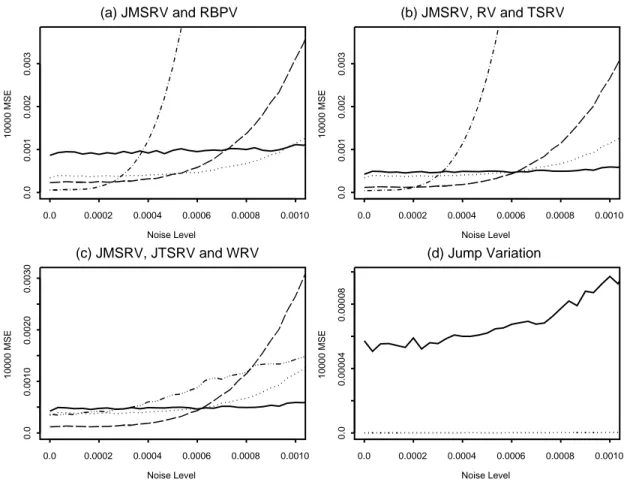
Noise Level 10000 MSE 0.0 0.0002 0.0004 0.0006 0.0008 0.0010 0.0 0.001 0.002 0.003 (a) JMSRV and RBPV Noise Level 10000 MSE 0.0 0.0002 0.0004 0.0006 0.0008 0.0010 0.0 0.001 0.002 0.003 (b) JMSRV, RV and TSRV Noise Level 10000 MSE 0.0 0.0002 0.0004 0.0006 0.0008 0.0010 0.0 0.0010 0.0020 0.0030 (c) JMSRV, JTSRV and WRV Noise Level 10000 MSE 0.0 0.0002 0.0004 0.0006 0.0008 0.0010 0.0 0.00004 0.00008 (d) Jump Variation
Figure 2: MSE (multiplied by 104) plots for continuous price process (no jumps). (a)
MSE using JMSRV (dotted curve) and RBPV based on all data (dot-dash curve) and 5-minute (dash curve) and 15-5-minute (solid curve) subsampled data. (b) MSE using JMSRV (dotted curve), RV(dot-dashed curve) and TSRV with K = 5 (dashed curve) and K = 15 (solid curve). (c) MSE using JMSRV (dotted curve), JTSRV with K = 5 (dashed curve) and K = 15 (solid curve) and WRV (dot-dashed curve). (d) MSEs of Jump variation estimation using RBPV (solid curve) and wavelets (dotted curve).
wavelet is different from TSRV. JTSRV was evaluated with K being 5 and 15, which
corresponds to 5- and 15-minute returns, respectively. We computed WRV using
wavelet coefficients at the first 8 levels. JMSRV was computed with M = 11 and
Km = 5,· · ·,15. To demonstrate the performances of the proposed estimators we compared them with RBPV, RV and TSRV estimators directly applied to the same data without jump adjustments. RBPV was evaluated for all data and subsampled
Noise Level 10000 MSE 0.0 0.0002 0.0004 0.0006 0.0008 0.0010 0.0 0.002 0.004 0.006 (a) JMSRV and RBPV Noise Level 10000 MSE 0.0 0.0002 0.0004 0.0006 0.0008 0.0010 0.0 0.02 0.04 0.06 0.08 (b) JMSRV, RV and TSRV Noise Level 10000 MSE 0.0 0.0002 0.0004 0.0006 0.0008 0.0010 0.0 0.001 0.003 0.005 (c) JMSRV, JTSRV and WRV Noise Level 10000 MSE 0.0 0.0002 0.0004 0.0006 0.0008 0.0010 0.0 0.0005 0.0010 0.0015 (d) Jump Variation
Figure 3: MSE (multiplied by 104) plots for price process with one jump. The same
captions as those in Figure 2 are used.
data corresponding to 5- and 15-minute returns, RV was computed based on all data,
and TSRV was applied with K = 5 and 15 partition groups corresponding to 5- and
15-minute returns, respectively.
We plotted the MSEs of the estimators against noise level for continuous price process (no jumps) in Figure 2, and for the price process with one and three jumps, respectively, in Figures 3 and 4. In each of Figures 2-4, (a), (b) and (c) plot the MSEs of RBPV, RV and TSRV, and JTSRV and WRV, respectively, along with the MSE of
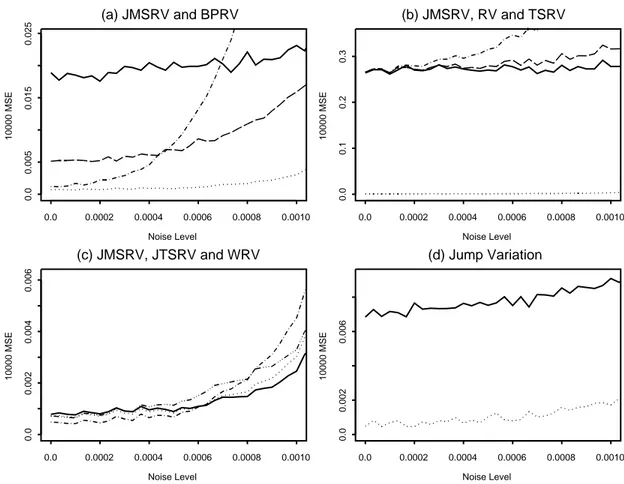
Noise Level 10000 MSE 0.0 0.0002 0.0004 0.0006 0.0008 0.0010 0.0 0.005 0.015 0.025 (a) JMSRV and BPRV Noise Level 10000 MSE 0.0 0.0002 0.0004 0.0006 0.0008 0.0010 0.0 0.1 0.2 0.3 (b) JMSRV, RV and TSRV Noise Level 10000 MSE 0.0 0.0002 0.0004 0.0006 0.0008 0.0010 0.0 0.002 0.004 0.006 (c) JMSRV, JTSRV and WRV Noise Level 10000 MSE 0.0 0.0002 0.0004 0.0006 0.0008 0.0010 0.0 0.002 0.006 (d) Jump Variation
Figure 4: MSE (multiplied by 104) plots for price process with three jumps. The same
captions as those in Figure 2 are used. the presentation.
For the case of continuous price process, Figure 2 shows that, when there is no microstructure noise or noise level is very low, RV and RBPV based on all data are the best. However, they are very sensitive to noise. As the noise level increases, their performances quickly deteriorate, and they are overwhelmingly dominated by TSRV, MSRV, JTSRV, JMSRV and WRV estimators. For the subsampling based estimators, the higher the noise level is, the lower the subsampling frequency that should be used to make their MSEs smaller. Generally the MSEs of MSRV and JMSRV are between
those of TSRV and JTSRV for 5- and 15-minute returns, respectively. In this case MSRV and JMSRV have almost the same MSE value. TSRV, MSRV, JTSRV, JMSRV and WRV are noise resistant and have comparable performance, but none achieve the smallest MSE uniformly over the entire range of the noise level.
For the case of price process with jumps, Figures 3 and 4 demonstrate that the proposed estimators outperforms all existing estimators. RV, TSRV and MSRV are very sensitive to jumps. In this case, it is necessary to remove the jumps first before calculating the estimated integrated volatility. Regardless of noise level, one jump in the price process is enough to destroy RV, TSRV and MSRV whose MSEs are far larger than those of JTSRV, JMSRV and WRV. This is clearly demonstrated by the fact that the MSE of MSRV is between those of TSRV estimators and the rescaled
MSEs of RV and TSRV in Figure 3(b) have values far above 0.04, while the rescaled
MSEs of the proposed JMSRV, JTSRV and WRV in Figure 3(c) are close to 0.001.
In the case of one jump, Figures 3(a) and 3(c) imply that RBPV based estimators generally have larger MSEs than the proposed JMSRV, JTSRV and WRV. RBPV is proposed to handle jumps for data without noise. For very low noise levels, RBPV for all data has slightly less MSE than the JMSRV. But as noise level increases, its MSE increases dramatically, with MSE values many times larger than that of the JMSRV. When the price process has three jumps, Figures 4(a) and 4(c) indicate that the proposed estimators obviously outperforms RBPV based estimators at all noise levels, and again Figure 4(b) suggests that the behaviors of RV, TSRV and MSRV estimators are completely ruined by the jumps.
For the estimation of jump variation Ψ in the jump-diffusion price model, we
with the existing estimator in Barndorff-Nielsen and Shephard (2006), which is the
difference of RV andπ/2 of RBPV of order (1,1). We evaluated the existing estimator
based on all and subsampled data and found that the MSEs are very close. Figures 3(d) and 4(d) plot, against noise level, the MSEs of the proposed estimator and the existing estimator based on 5-minute returns for one and three jumps, respectively. When jumps are present in the log price process, we have also checked the number of estimated jumps. The percentage of finding correct number of jumps ranges from 90% to 99% over the noise level. For the continuous price case, there is no jump and the jump variation is zero. To check the performances of the proposed estimator and the existing estimator in this case, we have plotted their MSEs in Figure 2(d). All plots show that the proposed estimators have excellent performance and are overwhelmingly better than the existing estimator.
The noise level relative to asset price found in high frequency data typically ranges
from 0.001% to 0.01%. We take the ratio of η2 and average integrated volatility
as a crude proxy for the relative noise level in the simulated model and find that
η ∈ [0,0.001] in the simulation plots closely matches with the range of the relative
noise level observed in real data. Indeed, since the Ornstein-Uhlenbeck process for
logσ2
t has a normal stationary distribution with mean−6.8020 and variance 0.3125,
under this stationary distribution the expected integrated volatility R01E[σ2
t]ds is
equal to 0.0012995; The requirement of the proxy η2/0.0012995 ∈[0.001%,0.01%] is
translated into η∈[0.014%,0.14%], which is close toη ∈[0,0.001]. Actually we have
tried on over a much more wide range of values for η. It turns out that the plotted
figures with η ∈ [0,0.001] display all MSE patterns found over the wide range of η
5.2
Applications
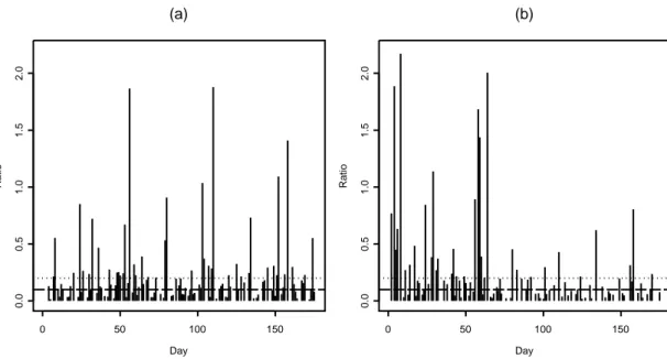
We have applied the proposed methods to two exchange rate data sets: one minute Euro-dollar and Yen-dollar exchange rates for the first seven months in 2004. The data sets were obtained from Quickstars, L. L. C., Connecticut, U.S.A. Figures 5(a) and 6(a) show the plots of the two exchange rate data. We applied our jump estimation to the exchange rate data for each day and plotted the estimated number of daily jumps in Figures 5(b) and 6(b). The plots show that jumps occur very often in the exchange rates. We computed WRV and the proposed estimator of jump variation for each day and plotted the estimated daily integrated volatility and jump variation in Figures 5(c-d) and 6(c-d). For these two data sets, jump variations often make significant contribution to total variations. To quantify the contribution, we calculated the ratios of the daily estimated jump variations and the daily integrated volatilities and plotted them in Figure 7. The percentages of days with jump variation exceeding 10% and 20% of integrated volatility are, respectively, 41% and 24% for Euro-dollar exchange rates and 30% and 19% for Yen-dollar exchange rates. For several days, the estimated jump variations even surpass the estimated integrated volatilities. This shows that ignoring jump effect in volatility estimation can inflate the volatility substantially.
6
Conclusions
We develop nonparametric methods to estimate jumps and jump variations for noisy data from a jump-diffusion model. With the estimated jumps we adjust data for jumps and then propose to apply TSRV and MSRV to the jump adjusted data for the estimation of integrated volatility. We also construct WRV from the jump
ad-Time Exchange rate 0 50000 100000 150000 200000 1.18 1.22 1.26 (a) Day Number of jumps 0 50 100 150 2 4 6 8 10 (b) Day Volatility 0 50 100 150 0.0 0.00010 0.00020 (c) Day Jump variation 0 50 100 150 0.0 0.00010 0.00020 (d)
Figure 5: (a) Euro-dollar exchange rates from January to July, 2004. (b) The number of
estimated jumps in each day. (c) Estimated daily integrated volatility. (d) Estimated daily jump variation.
justed data to estimate integrated volatility. Asymptotic theory established for the proposed estimators shows that the integrated volatility can be estimated under the jump-diffusion model asymptotically as well as under the continuous diffusion model. Simulations demonstrate that the proposed estimators have comparable performance with existing methods for either noisy data from the continuous diffusion model or noiseless data from the jump-diffusion model, but they outperform existing meth-ods when data contains jumps. An application of the jump and volatility estimation methods to two high-frequency Euro-dollar and Yen-dollar exchange rate data reveals
Time Exchange rate 0 50000 100000 150000 200000 0.00104 0.00108 0.00112 (a) Day Number of jumps 0 50 100 150 2 4 6 8 10 (b) Day Volatility 0 50 100 150 0.0 0.5 1.0 1.5 2.0 2.5 (c) Day Jump variation 0 50 100 150 0.0 0.5 1.0 1.5 2.0 2.5 (d)
Figure 6: (a) Japanese Yen-dollar exchange rates from January to July, 2004. (b) The
number of estimated jumps in each day. (c) Estimated daily integrated volatility. (d) Estimated daily jump variation.
important information in the exchange rates.
The paper initiates a new research direction on jump and volatility estimation in the field of high-frequency financial data. The proposed methods will stimulate more research on multiscale methods. For example, the paper leaves some issues and raises interesting problems for future investigation. They include asymptotic theory of WRV under smooth wavelets, the performance of the proposed methods for data with infinitely many jumps modeled by L´evy processes, characterization of log price process whose sample path has sparse representations under wavelets and other bases, and
Day Ratio 0 50 100 150 0.0 0.5 1.0 1.5 2.0 (a) Day Ratio 0 50 100 150 0.0 0.5 1.0 1.5 2.0 (b)
Figure 7: The ratios of estimated daily jump variations and integrated volatilities for (a)
Euro-dollar and (b) Japanese Yen-dollar exchange rates. Two horizontal lines are at 10% and 20% levels.
refinement of WRV with thresholding techniques to take full advantage of bases used.
7
Technical conditions and Proofs
We first state the technical conditions on model (1) and (2) that are needed for the technical proof and then outline the proofs of the results.
(A1). Wavelets (ψ, φ) used in jump estimation are differentiable.
(A2). µt and σt2 are continuous int almost surely and satisfy
E µ max 0≤t≤1µ 2 t ¶ <∞, E µ max 0≤t≤1σ 2 t ¶ <∞.
(A3). For the jump part of Xt in [0,1], its jump locations τ` and jump sizes L` obey
(A4). (µt, σ2t, Wt), (Nt, L`) and εt are independent. εt are i.i.d. with E(ε4t)<∞.
(A5). The continuous part ofXtis an Itˆo process, with (µt, σt) adapted to the complete
filtration generated by Brownian motion Wt.
Proof of Theorem 1. It is easy to show that the following inequality holds for any d >0, P ³ |Ψˆ −Ψ|> d n−1/4 ´ ≤P ³ ˆ q =q,|Ψˆ −Ψ|> d n−1/4 ´ +P(ˆq6=q).
From (4) we have that limn→∞P(ˆq6=q)→0. Hence,
lim d→∞nlim→∞P ³ |Ψˆ −Ψ|> d n−1/4´≤ lim d→∞nlim→∞P ³ ˆ q =q,|Ψˆ −Ψ|> d n−1/4´. (9) With ˆq=q, we have ˆ Ψ−Ψ = q X `=1 n ˆ L2` −L2` o = q X `=1 © Π2n,`+ Πn,`L` ª , (10) where Πn,` = ˆL`−L` = ( ¯Yˆτ`+−Y¯τˆ`−)−(Xτ`−Xτ`−). (11)
We state Claim I (with proof given late) that for each `,
Πn,` =OP(n−1/4). (12)
Claim I and L` = OP(1) imply that for each `, Πn,`L` = OP(n−1/4) and Π2n,` =
OP(n−1/2). Using these results we can show Claim II (with proof given late) that
q X `=1 |Πn,`L`|=OP(n−1/4), q X `=1 Π2 n,` =OP(n−1/2), that is, lim d1→∞nlim→∞P Ã q X `=1 |Πn,`L`|> d1n−1/4 ! = 0, (13) lim d1→∞nlim→∞P Ã q X Π2n,` > d1n−1/2 ! = 0. (14)
Putting together (10), (13) and (14) we deduce P ³ ˆ q =q,|Ψˆ −Ψ|> d n−1/4´≤P Ã q X `=1 © Π2 n,`+|Πn,`L`| ª > d n−1/4 ! ≤P Ã q X `=1 Π2n,` > d n−1/4/2 ! +P Ã q X `=1 |Πn,`L`|> d n−1/4/2 ! →0,
as n and then d sequentially go to infinity. Combining the above result with (9) we
derive that ˆΨ−Ψ is OP(n−1/4).
Now we need to prove Claim I stated in (12) and Claim II given by (13)-(14). First we prove (13)-(14) using (12). Because of similarity, we give arguments only for
(13). As q=N1 is a finite non-negative discrete random variable, we have
P Ã q X `=1 |Πn,`L`|> d1n−1/4 ! ≤P(N1 > m) +P Ã m X `=1 |Πn,`L`|> d1n−1/4, N1 ≤m ! ≤P(N1 > m) +P Ã m X `=1 |Πn,`L`|> d1n−1/4 ! ≤P(N1 > m) + m X `=1 P µ |Πn,`L`|> d1 m n −1/4 ¶ .
In above inequality we fix m, sequentially let n and thend1 go to infinity, and yield
the following inequality, lim d1→∞nlim→∞P Ã q X `=1 |Πn,`L`|> d1n−1/4 ! ≤P(N1 > m), (15)
where we have used the facts that Πn,`L` = OP(n−1/4) for each `, which we have
derived right after Claim I, and by definition it infers that for fixed m and `,
lim d1→∞nlim→∞P µ |Πn,`L`|> d1 mn −1/4 ¶ = 0.
The left hand side of (15) is free of m and N1 is finite. Letting m goes to infinity
in (15), we obtain lim d1→∞nlim→∞P Ã q X `=1 |Πn,`L`|> d1n−1/4 ! ≤ lim m→∞P(N1 > m) = 0,
which shows (13). The same arguments can be used to prove (14).
The proof left is to show Claim I of (12). Because of similarity, we prove the claim
for `= 1. Denote bym± the number ofti in ˆI+ = [ˆτ1,τˆ1+δn] and ˆI−= [ˆτ1−δn,τˆ1),
respectively. Then |m+−m−| ≤2,m+∼m−∼n1/2, and
¯ Yτˆ1+ = 1 m+ X ti∈I+ˆ Yti, Y¯τˆ1− = 1 m− X ti∈Iˆ− Yti.
AsYt contains noise, drift, diffusion and jump terms, denote byUi the differences
between the two averages over ˆI± for the four terms, respectively. Then,
( ¯Yτˆ1+−Y¯τˆ1−)−(Xτ1 −Xτ1−) =
4
X
i=1
Ui−LNτ1, (16)
and it is enough to show that U1, U2, U3, andU4−LNτ1 are OP(n−1/4).
First of all, let us consider the noise term. U1 is the difference of two averages of
m+andm−i.i.d. random variables εt, respectively, soU1 has mean zero and variance
η2(m−1
+ +m−−1) =O(n−1/2). Hence, U1 =OP(n−1/4).
Next, consider drift term. Use Condition (A2), it is easy to see that U2 = 1 m+ X ti∈I+ˆ Z ti ˆ τ1 µsds− 1 m− X ti∈Iˆ− Z τˆ1 ti µsds = 1 m+ OP Ãm + X i=1 i/n ! + 1 m− OP Ãm − X i=1 i/n ! =OP(n−1/2).
Third, consider the continuous diffusion term. Note that U3 = 1 m+ X ti∈I+ˆ Z ti τ1−2δn σsdWs− 1 m− X ti∈Iˆ− Z ti τ1−2δn σsdWs. (17)
Let I+ = [τ1, τ1+δn] andI− = [τ1−δn, τ1). We will replace ˆI± in above summation
indices by I±, respectively, and show that the resulting difference satisfies
X Z ti τ1−2δn σsdWs− X Z ti τ1−2δn σsdWs =OP(n−1/4 log5/2 n). (18)
Because of similarity, we prove (18) for the case of ˆI+andI+. The difference between P ti∈I+ˆ Rti τ1−2δnσsdWs and P ti∈I+ Rti
τ1−2δnσsdWs involves those terms
Rti
τ1−2δnσsdWs
withtifalling to exact one of the two intervals ˆI+andI+. Since ˆτ1−τ1isOP(n−1 log2 n),
the total number of such terms isOP(log2 n). We get (18) by multiplyingOP(log2 n)
with OP(n−1/4 log1/2 n), the order in probability for
Rti
τ1−2δnσsdWs, which can be
es-tablished as follows. Because of Condition (A4), (σ, W) and τ1 are independent, and
hence conditioning on τ1,
nRt
τ1−2δnσsdWs, t ≥τ1−2δn
o
is a martingale. We apply the maximal martingale inequality (Kloeden and Platen 1999, equation 3.6 in section 2.3) to the martingale and use (4) and Condition (A2) to obtain
P µ max ½¯¯ ¯ ¯ Z ti τ1−2δn σsdWs ¯ ¯ ¯ ¯, ti ∈Iˆ+∪ I+ ¾ > n−1/4 log1/2 n ¶ ≤P µ max τ1−δn≤ti≤τ1+2δn ¯ ¯ ¯ ¯ Z ti τ1−2δn σsdWs ¯ ¯ ¯ ¯> n−1/4 log1/2 n ¶ +P(|ˆτ1−τ1|> δn) = E µ P · max τ1−δn≤ti≤τ1+2δn ¯ ¯ ¯ ¯ Z ti τ1−2δn σsdWs ¯ ¯ ¯ ¯> n−1/4 log1/2 n ¯ ¯ ¯ ¯τ1 ¸¶ +o(1) ≤E à 1 n−1/2 log nE "µZ τ1+2δn τ1−2δn σsdWs ¶2¯¯ ¯ ¯ ¯τ1 #! +o(1) = 1 n−1/2 log n Z 2δn −2δn E¡στ21+s¢ ds+o(1)≤E µ max 0≤t≤1σ 2 t ¶ O(log−1 n) +o(1) →0,
as n→ ∞. Substituting (18) into (17) we obtain
U3 = 1 m+ X ti∈I+ Z ti τ1−2δn σsdWs− 1 m− X ti∈I− Z ti τ1−2δn σsdWs+OP(n−3/4 log5/2 n). (19)
Denote by Pτ, Eτ and V arτ conditional probability, mean, and variance given τ1.
Note that τ1 is independent of (σ, W). Given τ1, for |ti−τ1| ≤δn,
Rti
τ1−2δnσsdWs has
conditional mean zero and conditional covariance
Eτ µZ ti τ1−2δn σsdWs Z tj τ1−2δn σsdWs ¶ = Z ti∧tj τ1−2δn E(σ2 s)ds≤(ti∧tj−τ1+2δn) max 0≤s≤1E ¡ σ2 s ¢ .
Hence, it is easy to compute the following conditional mean and variance 1 m+ X ti∈I+ Eτ Z ti τ1−2δn σsdWs = 1 m− X ti∈I− Eτ Z ti τ1−2δn σsdWs = 0, (20) Varτ 1 m+ X ti∈I+ Z ti τ1−2δn σsdWs− 1 m− X ti∈I− Z ti τ1−2δn σsdWs ≤ 3 m+ X ti∈I+ Z ti τ1−2δn E(σ2 s)ds+ 4 m− X ti∈I− Z ti τ1−2δn E(σ2 s)ds ≤4 max 0≤s≤1E(σ 2 s) Ã 4δn+ 1 m+ m+ X i=1 i/n+ 1 m− m− X i=1 i/n ! =O(n−1/2). (21)
Equations (20) and (21) together with Tchebysheff’s inequality imply that the
differ-ence of the first two terms on the right hand side of (19) is OP(n−1/4) under Pτ, and
hence it is OP(n−1/4). This result together with (19) shows that U
3 =OP(n−1/4).
Finally, we consider the jump term. Denote by Ω1,n the event min{τ`−τ`−1, ` =
1,· · · , q}>2δn(τ0 = 0) and Ω2,n the event|τˆ`−τ`| ≤n−1 log2 nfor` = 1,· · · , q= ˆq,
and let Ωn = Ω1,n∩Ω2,n. Condition (A3) implies that min{τ`−τ`−1, `= 1,· · · , q}is
positive almost surely, and then limn→∞P(Ω1,n) = P(min{τ`−τ`−1, `= 1,· · · , q}>0)
= 1. Also (4) implies limn→∞P(Ω2,n) = 1. Hence limn→∞P(Ωn) = 1. On Ωn,
|τˆ1−τ1| ≤n−1 log2 n and the distances between any two jumps ofXt are great than
2δn, so ifXtjumps on the interval [ˆτ1±δn], it can jump only once and atτ1 ∈[ˆτ1±δn].
Thus, we have U4 = 1 m+ X ti∈I+ˆ Nti X `=1 L`− 1 m− X ti∈Iˆ− Nti X `=1 L` is equal to LNτ1 [1−n(τ1−τˆ1)/m+] if ˆτ1 ≤τ1 andLNτ1 [1−n(ˆτ1−τ1)/m−] if ˆτ1 > τ1. We conclude that on Ωn |U4−LNτ1| ≤ |LNτ1|(m − ++m−−1)n|τˆ1−τ1| ≤ |LNτ1|(m − ++m−−1) log2 n.
By considering it on Ωn and Ωcn we obtain P(|U4−LNτ1|> n −1/2 log3 n)≤P(Ωc n) +P ¡ Ωn∩ © |U4−LNτ1|> n −1/2 log3 nª¢ ≤P(Ωc n) +P ¡ (m− ++m−−1)|LNτ1|> n −1/2 log n¢→0, as n→ ∞,
that is, U4−LNτ1 =OP(n−1/2 log
3 n) = o
P(n−1/4).
Proof of Theorem 2. X has q=N1 jumps atτ`, `= 1,· · · , q. Let Xd t = Nt X `=1 L` = X τ`≤t L`
be the jump part of X. With the continuous parts of Xt and Yt defined in (8), we
yield Xt= Xtc+Xtd and Yt =Ytc+Xtd. From the definition of the data adjustment
in (6) and (7), we conclude Y∗ ti+K −Y ∗ ti =Y c ti+K −Y c ti+ X ti<τ`≤ti+K L`− X ti<ˆτ`≤ti+K ˆ L` ≡Ytci+K −Y c ti +ξi. (22)
Similar to the jump part proof of Theorem 1, denote by Ωnthe event min{τ`−τ`−1, ` =
1,· · · , q}> K/n and |τ`ˆ −τ`| ≤n−1 log2 n for` = 1,· · · , q= ˆq. Condition (A3) and
(4) imply limn→∞P(Ωn) = 1. So it is enough to show that [Y∗, Y∗](K)−[Yc, Yc](K)
on Ωn isOP(n−1/4+K−1 log2 n).
Note that on Ωn, first Xt has at most one jump in each of intervals [ti, ti+K] of
lengthK/n; second, since (K/n)/(n−1 log2 n) = K/log2 n→ ∞, in comparison with
intervals [ti, ti+K], the interval formed by each pair τ` and ˆτ` is tiny. Thus, on Ωn,
there are only three cases for the relationship between the two types of intervals: (i) ti, ti+K < τ`,τˆ` orti, ti+K > τ`,τˆ`;
(ii) ti < τ`,τˆ` < ti+K, and for each (τ`,τˆ`) there is at most n(K/n− |τ`−τˆ`|)≤K
(iii) either ti or ti+K (but not both) is between τ` and ˆτ`, and for each (τ`,τˆ`) there
is at most 2n|τ`−τˆ`| ≤2 log2 n such intervals [ti, ti+K].
Under the aforementioned three cases, ξi on Ωn is equal to 0,L`−L`ˆ , andL` or−L`ˆ ,
respectively. Hence from (22) we have that for Cases (i), (ii) and (iii), (Y∗
ti+K−Y ∗ ti) 2− (Yc ti+K −Y c ti)
2 is, respectively, equal to zero, and O
P(|L` −Lˆ`|) and OP(|L`|+|Lˆ`|).
From the expression of ASRV in Section 4.1 we have
[Y∗, Y∗](K)−[Yc, Yc](K) = 1 K nX−K i=1 h (Y∗ ti+K −Y ∗ ti) 2−(Yc ti+K −Y c ti) 2i.
Classifying aboven−K summation terms according to intervals [ti, ti+K] in Cases (i),
(ii) and (iii), we can bound [Y∗, Y∗](K)−[Yc, Yc](K) on Ω
n by multiplying the bounds
of (Y∗ ti+K −Y ∗ ti) 2 −(Yc ti+K −Y c ti)
2 with the corresponding total numbers of intervals
[ti, ti+K] under the three cases and then dividing by K. With zero difference for Case
(i), we need to do multiplications only for Cases (ii) and (iii), where the bounds and
the total numbers are available. The resulting bound for [Y∗, Y∗](K)−[Yc, Yc](K) on
Ωn is OP(Hn,K), where Hn,K = q X `=1 |L`−Lˆ`|+ 2K−1 log2 n q X `=1 (|L`|+|Lˆ`|).
Conditions (A3) and Theorem 1 imply thatPq`=1|L`−Lˆ`|=OP(n−1/4) and
Pq
`=1(|L`|+
|Lˆ`|) = OP(1), so Hn,K =OP(n−1/4+K−1 log2 n), which is the order in probability
for [Y∗, Y∗](K)−[Yc, Yc](K) on Ω
n. The proof is complete.
Proof of Theorem 3. Define ˆ
ΘcK = [Yc, Yc](K)− 1
K[Y
c, Yc](1),
the TSRV estimator of Θ for the continuous diffusion price model. The theorem 4
standard normal random variable multiplied by Υ. Since convergence stably in law is stronger than convergence in law, and
ˆ ΘK−ΘˆcK = [Y∗, Y∗](K)−[Yc, Yc](K)+ 1 K © [Y∗, Y∗](1)−[Yc, Yc](1)ª,
the theorem is proved if we show two assertions,
[Y∗, Y∗](K)−[Yc, Yc](K) =o p ¡ n−1/6¢, ¡ [Y∗, Y∗](1)−[Yc, Yc](1)¢/K =o p ¡ n−1/6¢.
The first assertion follows from an immediate application of Theorem 2 with K =
c n2/3. Because of K ∼n2/3, the second assertion is a consequence of
[Y∗, Y∗](1)−[Yc, Yc](1)=OP(n1/4 log n). (23)
The rest of the proof is to show (23). Note that the unadjusted data Yti contain
q =N1 jumps with jump sizes L`, and ˆq jumps with jump sizes ˆL` are added in the
adjusted data Y∗. Hence, the increments of Y∗ and Yc over [t
i, ti+1] satisfy Y∗ ti+1−Y ∗ ti = (Y c ti+1−Y c ti)+ X ti<τ`≤ti+1 L`− X ti<ˆτ`≤ti+1 ˆ L` ≡(Ytci+1−Y c ti)+ξi, i= 1,· · · , n−1.
Of these (n−1) intervals [ti, ti+1], at leastn−1−(ˆq+q) of them don’t contain τ` or
ˆ
τ`, and thus their corresponding ξi are zero. The number of non-zero ξi are at most
(ˆq+q), and these non-zero ξi are equal toL`−L`ˆ , L`, or−L`ˆ , depending on both or
just one of ˆτ` and τ` falling into [ti, ti+1]. Therefore,
|[Y∗, Y∗](1)−[Yc, Yc](1)| ≤2 q X `=1 L2` + 2 ˆ q X `=1 ˆ L2` + 4 max 1≤i≤n|Y c ti| ( q X `=1 |L`|+ ˆ q X `=1 |L`ˆ | ) .
We prove (23) by establishing OP(n1/4 log n) for above bound as follows.
First,Pq`=1|L`|, Pq `=1L2`, Pqˆ `=1Lˆ2` and Pqˆ
`=1|Lˆ`| all areOP(1); second,
max 1≤i≤n|Y c ti| ≤1max≤i≤n{|X c ti|+|εti|} ≤ max 0≤t≤1|X c t|+ max1≤i≤n|εti|;