A Randomized Linear Programming Method for
Network Revenue Management with Product-Specific No-Shows
Sumit Kunnumkal
Indian School of Business, Gachibowli, Hyderabad, 500032, India sumit [email protected]
Kalyan Talluri
ICREA and Universitat Pompeu Fabra, Barcelona, 08005, Spain [email protected]
Huseyin Topaloglu
School of Operations Research and Information Engineering, Cornell University, Ithaca, New York 14853, USA
May 19, 2011
Abstract
Revenue management practices often include overbooking capacity to account for customers who make reservations but do not show up. In this paper, we consider the network revenue management problem with no-shows and overbooking, where the show-up probabilities are specific to each product. No-show rates differ significantly by product (for instance, each itinerary and fare combination for an airline) as sale restrictions and the demand characteristics vary by product. However, models that consider no-show rates by each individual product are difficult to handle as the state-space in dynamic programming formulations (or the variable space in approximations) increases significantly. In this paper, we propose a randomized linear program to jointly make the capacity control and overbooking decisions with product-specific no-shows. We establish that our formulation gives an upper bound on the optimal expected total profit and our upper bound is tighter than a deterministic linear programming upper bound that appears in the existing literature. Furthermore, we show that our upper bound is asymptotically tight in a regime where the leg capacities and the expected demand is scaled linearly with the same rate. We also describe how the randomized linear program can be used to obtain a bid price control policy. Computational experiments indicate that our approach is quite fast, able to scale to industrial problems and can provide significant improvements over standard benchmarks.
Introduction
Revenue management controls the sale of a perishable product to a heterogeneous population of customers with different valuations for the same product. The physical product could be hotel rooms, airline seats or media advertising slots sold at a specific price with sale restrictions. Typically, the products are defined over a network and firms have to control the sale of multiple products that consume different bundles of resources. For example, airlines products are itineraries that span different flight legs, while hotel customers stay for multiple nights using the inventory over different days.
Revenue management practices often include overbooking capacity to account for customers who make reservations but do not show up. No-show rates differ significantly by product as sale restrictions, time-of-purchase and demand characteristics vary by product. However, models that consider no-show rates by each individual product are difficult to handle as the state-space in dynamic programming formulations or the variable space in approximations increases significantly. In this paper, we develop tractable models for jointly making the capacity control and overbooking decisions in network revenue management problems with product-specific no-shows.
While the problem setting is applicable to a wide range of industries, we use airline terminology throughout the paper for concreteness. Thus, products are itinerary and fare-class combinations, where a fare-class represents a revenue management fare-product corresponding to a fare combined with some restrictions. The resources are the seats on the flight legs. The airline gets requests for the products for a future date and it has to decide in real time which of these product requests to accept and which to reject. In making this decision, the airline not only has to consider the uncertainty in the customer arrivals but also the fact that not all customers who make purchases show up at the time of departure of the flight. Because of these no-shows, the airline may choose to overbook and accept more itinerary requests than the capacity of the flight leg. However, by overbooking it also runs the risk of denying seats to customers with reservations, if the number that show up at the time of flight departure exceeds the seating capacity of the flight leg. Since the number of dimensions of the state variable quickly gets large in the dynamic programming formulations of practical problem instances, computing the optimal capacity control policy is generally intractable and one has to resort to heuristics that approximate the solution to the dynamic problem.
In this paper, we propose a randomized linear programming method for jointly making the capacity control and overbooking decisions in network revenue management problems with product-specific no-shows. In our approach, we generate samples of the demands for the products and the show-ups, and solve a two-stage linear stochastic program, where the first stage decisions are the number of reservation requests to accept and the second stage decisions are the number of denied boardings. It thus extends the randomized linear programming method of Talluri and van Ryzin (1999) to overbooking decisions with product-specific no-shows.
The approach that we propose has a number of appealing features. To begin with, it yields an upper bound on the optimal expected total profit and we show that this upper bound is tighter than the
one obtained by the deterministic linear program of Bertsimas and Popescu (2003). Having a tight upper bound on the optimal expected total profit becomes valuable when trying to assess the performance of approximate control policies. Moreover, there is evidence that methods obtaining tight upper bounds also tend to yield policies with good profit performance; see for example Topaloglu (2009b) and Talluri (2009). Also, by using samples of the random variables rather than their expected values, we are able to better capture the stochastic nature of the network revenue management problem; for instance, our model can accommodate arbitrary probability distributions for the demand random variables. As a result, we expect the randomized linear program to yield good control policies.
Another appealing feature of our approach is that the deterministic linear program proposed by Bertsimas and Popescu (2003) is, to our knowledge, the only tractable method to obtain upper bounds on the expected total profit. However, this approach assumes that all random variables take on their expected values and it does not consider the random nature of the demand and show-ups. Our randomized linear program closes this gap by providing a tractable method to obtain upper bounds on the optimal expected total profit, while considering the random nature of the demand and show-ups. Finally, the method that we propose requires solving only linear programs, leveraging the speed, robustness and parallelization of modern solvers. Therefore, our approach can be easily implemented using commercially available solvers and modeling languages with minimal customized coding, an attractive proposition for practicing revenue managers.
A control policy that is widely used in practice is a bid price control. In bid price control, we have a bid price for each flight leg, which is essentially a proxy for the expected marginal value of capacity for that flight leg. In this case, a bid price policy accepts a product request only if its fare exceeds the sum of the bid prices of the flight legs used by it. Traditionally, bid prices are computed by using the optimal values of the dual variables of the seat availability constraints in the deterministic linear programming formulation. By using samples of the random variables, our randomized linear program is able to obtain better estimates of the expected marginal value of capacity than the deterministic linear program. Consequently, we expect better profit performance from our randomized linear program. This is indeed the case in our computational experiments.
To summarize, we make the following research contributions in this paper. 1) We propose a new method to jointly make the capacity control and overbooking decisions in network revenue management problems with no-shows. Our method is sampling-based and thus flexible enough to model a wide variety of probability distributions for the random demand arrival processes. 2) We show that our method yields an upper bound on the optimal expected total profit and this upper bound is tighter than that obtained by the deterministic linear program. 3) We show that the upper bound on the expected total profit provided by our approach is asymptotically tight as we scale the capacities on the flight legs and the expected amount of demand linearly with the same rate. Furthermore, our proof also implies that the upper bound provided by the standard deterministic linear program is tight in the same asymptotic regime, which is a result that has not been established within the overbooking context. 4) Our computational experiments compare our randomized linear programming method with existing methods for a range of demand scenarios to test the upper bounds and revenue performance. Overall,
our approach is fast, easy to implement, numerically robust and scalable even for industrial problems and computational experiments indicate that the bid price policy obtained by our method can generate significantly higher profits than standard benchmarks.
1 Related work
A commonly used method to make the capacity control decisions over an airline network is the deterministic linear program; see Simpson (1989) and Williamson (1992) for a model without overbooking and Bertsimas and Popescu (2003) for an extension to handle no-shows and cancellations. The underlying assumptions of the deterministic linear program are that all random quantities take on their expected values and the number of reservation requests accepted and the number of denied boardings can be fractional. In this linear program, there is one constraint for each flight leg, which ensures that the total number of passengers that are eventually boarded does not exceed the capacity of the flight. The optimal values of the dual variables associated with the flight leg capacity constraints are usually used as proxies for the expected marginal values of each unit of capacity. These dual variables are used to control sales through a bid price policy. Erdelyi and Topaloglu (2009) show that the optimal objective value of the deterministic linear program is an upper bound on the optimal expected total profit.
Kleywegt (2001) develops a joint pricing and overbooking model over an airline network assuming that the reservation requests are deterministic. He solves the model by using duality and decomposition ideas. Karaesmen and van Ryzin (2004b) describe a capacity allocation and overbooking model that is useful when dealing with multiple flight legs that can serve as substitutes of each other. Similar to ours, their approach has a two stage stochastic programming flavor, but it is not clear how to extend their approach to general airline networks. Karaesmen and van Ryzin (2004a) develop a joint capacity allocation and overbooking model by using the deterministic linear program to estimate the revenue from the accepted reservations. Their approach uses a sequence of approximating assumptions, where the authors assume that the overbooking cost of a passenger can be prorated over the different flight legs and a reservation for an itinerary shows up for each flight in the itinerary independently.
Kunnumkal and Topaloglu (2008) and Erdelyi and Topaloglu (2009) formulate the overbooking problem over a network as a dynamic program with a high dimensional state vector. They approximate the value functions by separable functions and use the separable approximations to obtain control policies. Erdelyi and Topaloglu (2010) work with the same dynamic programming formulation and propose a dynamic programming decomposition approach to decompose the network problem into a number of single flight leg problems. However, since the single flight leg problem is intractable when there are product-specific no-shows, they have to resort to heuristics to approximately solve the single flight leg problems. Kunnumkal and Topaloglu (2011) propose a stochastic approximation algorithm to obtain bid prices. Their approach visualizes the expected total profit as a function of the bid prices and uses sample path-based gradients of the expected total profit function to search for a good set of bid prices in a stochastic approximation algorithm. This stochastic approximation algorithm eventually
computes high quality bid prices, but its run times can be long, it involves tuneable parameters that need to be adjusted with trial and error and it does not have a well-defined stopping condition. We use the approaches proposed by Karaesmen and van Ryzin (2004a) and Kunnumkal and Topaloglu (2011) as benchmarks in our computational experiments. Finally, the book by Talluri and van Ryzin (2004) contains background and details on revenue management, specifically the chapters on overbooking and network revenue management.
The rest of the paper is organized as follows. Section 2 formulates the network revenue management problem with no-shows as a dynamic program. Section 3 describes the deterministic linear program proposed by Bertsimas and Popescu (2003). Section 4 builds on this linear program to develop our randomized linear program. Section 5 establishes the asymptotic tightness of the upper bounds provided by our randomized linear program. Section 6 presents our computational experiments.
2 Problem Formulation
An airline network consists of a set ofm flights andnproducts (itinerary-fare class combinations). The physically available capacity on flight i is ci. The booking horizon consists of time periods 1,2, . . . , τ and all flights depart at time period τ + 1. We make the standard assumption that the time periods are fine enough so that there is at most one product request in each time period. The probability that there is a request for product j in time period t is pjt. Product j has a revenue fj associated with it and we denote the flights in the product byi∈j. Throughout, we index flights byi, products byjand time byt. We have to decide, in an on-line fashion, whether to accept a request for productj to obtain revenue fj or reject the request in anticipation of future higher revenue requests.
When we decide to accept a request, it becomes a reservation. Not all reservations show up at the time of departure of the flight legs and we letqjt be the probability that a reservation for productjmade at time periodtshows up at the time of departure. Knowing that only a portion of the reservations show up at the departure time of the flight legs, the airline overbooks. That is, it accepts more reservations than the capacity of the flight. If more reservations show up than the capacity of the flight, then the airline has to decide which of these reservations to deny boarding.
Productj can potentially consume (if a reservation for it is allowed boarding) one unit of capacity on all flights i∈ j, and we letaij = 1 if i ∈ j and aij = 0 otherwise. On the other hand, if we deny boarding to a reservation for product j, then we incur a denied-service penalty cost of θj. We have to decide which of the product requests to accept during the booking period and which of the accepted reservations to deny boarding at the time of departure of the flight legs, the goal being to maximize expected total profits. The expected total profit is given by the difference between the expected revenue obtained by accepting the product requests and the expected penalty cost of denied service.
We make the following assumptions in our model. We assume that the demands for the different products and the show-up decisions of the different reservations are independent of each other and across time periods. We assume that there are no cancellations (reservations that cancel prior toτ) and we
do not give refunds to the reservations that do not show up at the departure time. This is for ease of notation and all the development in the paper goes through with minor modifications in the presence of cancellations and refunds, provided that the cancellation decisions are independent across reservations and time periods. Finally, we assume that fj ≤θjqjt for each product j. This is again without loss of generality since if we have fj > θjqjt, then we can always make a profit in expectation by accepting a request for product j at time periodt and denying it boarding at the time of departure.
The decision problem is to determine (online, without knowing future demands) the product requests to accept, and at departure time, to determine which of the confirmed reservations to deny boarding. We let xjt be a binary variable equal to 1 if we accept a request for product j at time periodt and 0 otherwise. Since a reservation for productj at time period tshows up with probability
qjt, the show-up decision for a product j request at time period t can be written as Sjtxjt, where Sjt is a Bernoulli random variable with success probability qjt. Letting sjt be a realization of Sjt and
s={sjt:∀j, t}and x={xjt:∀j, t}, we represent the total denied-service cost as the solution to Π(s, x) = min n ∑ j=1 τ ∑ t=1 θjwjt (1) subject to n ∑ j=1 τ ∑ t=1 aij[sjtxjt−wjt]≤ci ∀i (2) wjt ≤sjtxjt ∀j, t (3) wjt ∈ {0,1} ∀j, t. (4)
In the above linear integer program, the decision variablewjt indicates whether or not we deny boarding to the confirmed reservation for product j purchased at time period t. The first set of constraints ensures that the total number of reservations that are eventually allowed to board does not exceed the capacity of the flight. The second set of constraints ensures that we can deny boarding only if the corresponding reservation shows up at the time of departure. Notice that we assume the airline has the ability to first observe the show-up demand for all the reservations and then decide which reservations to deny boarding. This is a somewhat stylized model of the actual deny-service process, where the airline may have to make the deny-service decisions online with partial information and many more restrictions. Nevertheless, following Bertsimas and Popescu (2003) and Erdelyi and Topaloglu (2009), we use problem (1)-(4) to approximately capture the overall denied-service costs.
Letxt={xjs:∀j, s= 1, . . . , t−1}denote the state of reservations in the system at the beginning of time period t = 2, . . . , τ+ 1 and let xt⊕ej denote the state of reservations in the system at the beginning of time periodt+ 1 given that we hadxtreservations in the system at the beginning of time periodtand we accepted a request for productj at time periodt. Similarly, letxt⊕0 denote the state of reservations in the system at the beginning of time period t+ 1 given that we hadxtreservations in the system at the beginning of time period tand we did not accept a request for any product at time periodt. The value functions {Vt(·) :∀t}are given by the optimality equation
Vt(xt) = n ∑ j=1 pjtmax { fj+Vt+1(xt⊕ej), Vt+1(xt⊕0) } +[1− n ∑ j=1 pjt ] Vt+1(xt⊕0) (5)
with the boundary condition thatVτ+1(xτ+1) =−E{Π(S, xτ+1)}. In this case,V1(¯0) denotes the optimal expected total profit at the beginning of the booking horizon, where ¯0 is an n-dimensional vector of zeros representing the fact that we start with 0 reservations. If the state of reservations at the beginning of time period t is xt, then it follows from (5) that it is optimal to accept a request for product j at time period tprovidedfj +Vt+1(xt⊕ej)≥Vt+1(xt⊕0).
In the optimality equation (5), the dimensionality of the state space increases exponentially with the number of products and the number of time periods. Therefore, solving this optimality equation quickly becomes computationally intractable. In the next two sections, we describe approximate methods that can be used to jointly make the capacity control and overbooking decisions.
3 Deterministic Linear Program
The deterministic linear program with overbooking and no-shows, proposed by Bertsimas and Popescu (2003), is given as zDLP = max n ∑ j=1 τ ∑ t=1 [fjyjt−θjwjt] (6) subject to n ∑ j=1 τ ∑ t=1 aij[qjtyjt−wjt]≤ci ∀i (7) yjt ≤pjt ∀j, t (8) wjt ≤qjtyjt ∀j, t (9) yjt, wjt ≥0 ∀j, t, (10)
where yjt represents the number of requests accepted for productj at time period tand wjt represents the number of these reservations that are denied boarding. The deterministic linear program assumes that of theyjt requests accepted, exactlyqjtyjtrequests show up at the time of departure. The first set of constraints ensures that the numbers of reservations that we allow boarding do not exceed the capacities of the flight legs. The second set of constraints ensures that the number of requests for product j that we accept at time period tdoes not exceed the expected number of product requests. The third set of constraints ensures that the numbers of reservations that we deny boarding do not exceed the expected numbers of reservations that show up at the time of departure. Thus, problem (6)-(10) assumes that all random quantities take on their expected values.
There are two uses of problem (6)-(10). First, Erdelyi and Topaloglu (2009) show that the optimal objective value of problem (6)-(10) provides an upper bound on the optimal expected total profit. That is, we have V1(¯0)≤zDLP. Upper bounds are useful when assessing the optimality gap of suboptimal policies. Second, we can use the optimal values of the dual variables corresponding to the flight leg capacity constraints as the bid prices. That is, letting µ={µi :∀i} be the optimal values of the dual variables corresponding to constraints (7), we accept a request for product j at time periodt if
fj ≥qjt m ∑ i=1
This is the bid price policy used by Bertsimas and Popescu (2003). Noting thatµi is an estimate of the marginal value of capacity on flight legiandqjt is the show-up probability, we can interpret the decision rule in (11) as accepting a product request only if its revenue exceeds the total expected marginal value of the capacities that it uses.
4 A Randomized Linear Program
The randomized linear program proposed by Talluri and van Ryzin (1999) is a tractable and attractive approach for making the capacity control decisions in the absence of no-shows. It is only natural that we try to extend the approach for jointly making the capacity control and overbooking decisions when we have no-shows. We propose solving the following optimization problem to obtain an upper bound on the optimal expected total profit. LetDjt be the random variable that denotes the number of requests for product j at time period t. Note that we haveE{Djt}=pjt. As before, let Sjt be a Bernoulli(qjt) random variable, sjt be a realization of Sjt and S = {Sjt : ∀j, t}, s = {sjt : ∀j, t}. To compute the denied service cost as a function of the show-ups and accepted reservations, we let
˜ Π(s, y) = min n ∑ j=1 τ ∑ t=1 θjwjt (12) subject to n ∑ j=1 τ ∑ t=1 aij[sjtyjt−wjt]≤ci ∀i (13) wjt ≤sjtyjt ∀j, t (14) wjt ≥0 ∀j, t, (15)
in which case, we approximate the expected total profit under a realizationdof demand arrivals as
zRLP(d) = max n ∑ j=1 τ ∑ t=1 fjyjt−E{Π(˜ S, y)} (16) subject to 0≤yjt ≤djt ∀j, t, (17) where d = {djt : ∀j, t} is a realization of the random variables D = {Djt : ∀j, t}. Note that ˜Π(·,·) is the linear programming relaxation of Π(·,·) and constraints (13)-(15) have the same interpretation as constraints (2)-(4). Note also that the optimal objective values of problems (12)-(15) and (16)-(17) respectively depend on the realizations of the random variables S and D. Finally, we can interpret
zRLP(d) as being the optimal profit when we make the accept or reject decisions for the product requests after observing a realizationdof the demands over the whole booking horizon.
LettingzRLP =E{zRLP(D)}, we show below thatzRLP is an upper bound on the optimal expected total profit and this upper bound is tighter than that obtained from the deterministic linear program. We begin with the following observations.
Lemma 1 1) Π(˜ s, y) is a convex function of s for a fixed y. 2) Π(˜ s, y) is a convex function of y for a fixed s.
Proof Parts (1) and (2) follow from standard linear programming theory as we can write ˜Π(s, y) with all sjtyjt terms on the right-hand side. Part (3) follows from the fact that ˜Π(·,·) is the linear programming relaxation of Π(·,·).
2
The next result shows that zRLP gives an upper bound on the optimal expected total profit.
Proposition 2 We haveV1(¯0)≤zRLP.
Proof Let ˆπ be an optimal policy to decide whether to accept or reject a product request at a time
period and let xπˆ(d) ={xπjtˆ(d)∈ {0,1}:∀j, t}denote the number of product requests that this optimal policy accepts along a sample path, where the argument d emphasizes that the number of accepted product requests depends on the sample d={djt :∀j, t}. We have
V1(¯0) =E {∑n j=1 τ ∑ t=1 fjxπjtˆ(D)−E{Π(S, xˆπ(D))|D} } ≤E{ n ∑ j=1 τ ∑ t=1 fjxπjtˆ(D)−E{Π(˜ S, xˆπ(D))|D} } ≤E{zRLP(D)}=zRLP, where the first equality follows from the optimality of the policy ˆπ, the first inequality uses the third part of Lemma 1 and the last inequality holds since xπˆ(d) is feasible but not necessarily optimal to problem (16)-(17).
2
We next show that the upper bound obtained by the randomized linear program is tighter than that obtained by the deterministic linear program. We need the following intermediate result. Let
ζ(d, s) = max n ∑ j=1 τ ∑ t=1 fjyjt−Π(˜ s, y) subject to 0≤yjt≤djt ∀j, t,
where d={djt :∀j, t} and s={sjt :∀j, t}. Note that we have ζ(p, q) = zDLP, where p={pjt :∀j, t} and q ={qjt :∀j, t} and we use the fact that−min{x}= max{−x}.
Lemma 3 For a fixeds, ζ(d, s) is a concave function of d.
Proof Let 0 ≤ α ≤ 1, and y1 and y2 be the optimal solutions to ζ(d1, s) and ζ(d2, s), respectively. We have that αy1 + (1−α)y2 is feasible to ζ(αd1+ (1−α)d2, s). Moreover, by the second part of Lemma 1, ˜Π(s, αy1+ (1−α)y2)≤αΠ(˜ s, y1) + (1−α) ˜Π(s, y2). It follows thatζ(αd1+ (1−α)d2, s)≥ ∑n
j=1 ∑τ
t=1fj[αyjt1 + (1−α)yjt2]−Π(˜ s, αy1+ (1−α)y2)≥αζ(d1, s) + (1−α)ζ(d2, s).
2
The following proposition shows that the randomized linear program obtains a tighter upper bound than the deterministic linear program.
Proof The first part of Lemma 1 and Jensen’s inequality imply that we have that E{Π(˜ S, y)} ≥ ˜
Π(E{S}, y) = ˜Π(q, y), where q ={qjt :∀j, t} and we use the fact thatSjt is Bernoulli(qjt). Therefore, we have ζ(d, q) ≥ max n ∑ j=1 τ ∑ t=1 fjyjt−E{Π(˜ S, y)} = zRLP(d) subject to 0≤yjt ≤djt ∀j, t,
where the equality is by the definition of zRLP(d) in problem (16)-(17). It follows that
zRLP =E{zRLP(D)} ≤E{ζ(D, q)} ≤ζ(E{D}, q) =zDLP,
where the second inequality uses Lemma 3 and Jensen’s inequality and the last equality holds since
E{Djt}=pjt.
2
As computing the upper bound E{zRLP(D)} analytically is difficult, we propose a simulation-based optimization scheme to approximate E{zRLP(D)}. We generate K samples of the random variables
D ={Djt :∀j, t} using Monte Carlo simulation. For each sample, we generate a further L samples of the random variables S = {Sjt :∀j, t}. That is, lettingdk ={dkjt :∀j, t} denote thekth sample ofD, we generate samples skl={skljt :∀j, t} forl= 1, . . . , L. We solve
zRLPk = max n ∑ j=1 τ ∑ t=1 fjyjtk − 1 L L ∑ l=1 n ∑ j=1 τ ∑ t=1 θjwkljt (18) subject to n ∑ j=1 τ ∑ t=1 aij[skljtykjt−wkljt]≤ci ∀i, l (19) wjtkl≤skljtykjt ∀j, t, l (20) ykjt≤dkjt ∀j, t (21) ykjt≥0 ∀j, t (22) wjtkl≥0 ∀j, t, l (23)
for the kth demand sample and use ∑Kk=1zk
RLP/K as an estimate of zRLP. Furthermore, letting
{ρkli : ∀i, l} be the optimal values of the dual variables corresponding to constraints (19), we use
ρi = ∑K
k=1 ∑L
l=1ρkli /K as the bid price for flight leg i and we accept a request for product j at time periodt only if fj ≥ m ∑ i=1 aijρi. (24)
In Appendix A, we show that zRLP is a concave function of the flight leg capacities by showing that it has a subgradient. Furthermore, we show that ρ ={ρi :∀i} is an estimate of the subgradient that we obtain from our sample. Therefore, we can interpret ρi as an estimate of the expected marginal value of capacity on flight leg i.
Note that comparing our acceptance rule in (24) with the acceptance rule in (11) of Bertsimas and Popescu (2003), (24) does not have the term qjt in it. This leads to increased robustness when the
actual deny-service process does not have full knowledge of no-shows. The acceptance rule in (11) can potentially accept very low fares which have low show-up probabilities. This is fine if we know that we can reject them in case of excess reservations, but this can turn out to be dangerous if at departure time we have to make deny decisions without knowing all the no-shows.
We close this section with two observations. First, since we have at most one product request arriving at each time period, we have at most one of the {dkjt : ∀j} being nonzero for each time period t. Consequently constraints (21) imply that at most τ of {yk
jt :∀j, t} are nonzero. Constraints (20) then imply that for each l = 1, . . . , L, we have at most τ of {wkljt : ∀j, t} nonzero. Therefore, problem (18)-(23) can be reduced to a linear program that has τ +τ L variables and (m+τ)L+τ
constraints. Second, it is possible to come up with an equivalent formulation of problem (18)-(23) by aggregating the denied boarding decisions for each product. In particular, we let wklj = ∑τt=1wkljt
and replace constraints (19) with the constraints ∑nj=1aij[ ∑τ
t=1skljtyjtk −wklj ]≤ci and constraints (20) with the constraints wklj ≤ ∑τt=1skljtyjtk. The resulting formulation has τ +nL decision variables and (m+n)L+τ constraints. The alternative formulation is more attractive whenn≤τ.
5 Asymptotic Optimality
In this section, we show that the upper bounds on the optimal expected total profit provided by our randomized linear program is asymptotically tight as the capacities on the flight legs and the expected demand scales linearly with the same rate. For models where all reservations show up at the departure time and overbooking is not possible, similar results have been shown for the deterministic linear program in Talluri and van Ryzin (1998) and for the randomized linear program in Topaloglu (2009a). Our results in this section can be visualized as generalizations of those results to the overbooking setting, but these generalizations are nontrivial due to the difficulties brought out by the possibility of overbooking.
We define a family of network revenue management problems {Pκ : κ ∈ Z+} indexed by the parameter κ with the following properties. (1) Problem Pκ has κτ time periods in the booking horizon. (2) In problemPκ, the probability that we get a request for productjat time periodtis given bypj⌈t/κ⌉, where⌈·⌉is the round up function. For notational brevity, we letpκjt =pj⌈t/κ⌉. (3) In problem
Pκ, a reservation for productjaccepted at time periodtshows up with probabilityq
j⌈t/κ⌉. Similar topκjt, for notational brevity, we letqjtκ =qj⌈t/κ⌉. As before, we assume that the arrivals and show-up decisions are independent across time periods. Furthermore, the show-up decisions of different reservations are independent. (4) In problem Pκ, the capacity on flight legiis κci.
With this definition of problemPκ, we observe that problemP1corresponds to the original network revenue management problem that we have been working with throughout the paper. The capacities on the flight legs in problemPκ areκ times the capacities on the flight legs in problemP1. Similarly, the length of the booking horizon in problem Pκ is κ times the length of the booking horizon in problem
P1. In addition, the probability of getting a request for productjat time periods 1,2, . . . , κin problem
similar observation holds for blocks of successive κ time periods over the booking horizon of problem
Pκ. In particular, for a fixed ℓ = 1, . . . , τ, the probability of getting a request for product j at time periods 1 + (ℓ−1)κ,2 + (ℓ−1)κ, . . . , κ+ (ℓ−1)κin problemPκis the same as the probability of getting a request for product j at time period ℓin problem P1. Thus, the expected total demand for product
j in problemPκ is κτ ∑ t=1 pκjt = κτ ∑ t=1 pj⌈t/κ⌉=κ τ ∑ t=1 pjt,
which implies that the expected total demand for product j in problem Pκ is κ times the expected total demand for product j in problem P1. Consequently, problem Pκ is a scaled version of problem
P1, where the leg capacities and the expected demand is scaled by the same factor κ. Intuitively, the parameter κ is a measure of how large the problem is and our goal is to show that the upper bound provided by our randomized linear program becomes tight as the problem gets larger.
We consider the deterministic linear program given by problem (6)-(10) for the network revenue management problem Pκ. Letting zDLPκ be the optimal objective value of the deterministic linear program for problem Pκ, we have
zDLPκ = max n ∑ j=1 κτ ∑ t=1 [fjyκjt−θjwκjt] (25) subject to n ∑ j=1 κτ ∑ t=1 aij[qκjtyκjt−wκjt]≤κci ∀i (26) yκjt≤pκjt ∀j, t (27) wjtκ ≤qκjtyκjt ∀j, t (28) yκjt, wκjt≥0 ∀j, t. (29) We let Vκ
1 (¯0) denote the optimal expected total profit for problem Pκ that we obtain by solving the corresponding dynamic program. Erdelyi and Topaloglu (2009) show that the optimal objective value of the deterministic linear program provides an upper bound on the optimal expected total profit. Therefore, we have zκDLP ≥V1κ(¯0)≥0, where the last inequality follows from the fact that the optimal expected total profit is nonnegative since rejecting all requests is a feasible policy with an optimal expected total profit of zero. This implies that if zDLPκ = 0, then we also have V1κ(¯0) = 0. Otherwise,
V1κ(¯0)/zDLPκ ≤ 1. In the next proposition, we show that this ratio converges to 1 as κ goes to infinity. In other words, as the problem size, measured by κ, increases, the optimal objective value of the deterministic linear program becomes a sharper and sharper estimate of the optimal expected total profit. We defer the proof of this result to Appendix B.
Proposition 5 We havelimκ→∞V1κ(¯0)/zDLPκ = 1.
It is interesting to observe that the proof of Proposition 5 in Appendix B also gives a policy to accept or reject the product requests and the ratio between the expected total profits obtained by this policy
and the optimal policy converges to 1. In particular, letting {yˆκjt :∀j, t} be the optimal values of the decision variables {yjtκ : ∀j, t} in problem (25)-(29), we can accept a request for product j at time periodtwith probability ˆyjtκ/pκjt. Noting constraints (27), ˆyjtκ/pκjt ∈[0,1] and we can indeed use ˆyjtκ/pκjt
as a probability. After making the acceptance decisions, we decide which show-ups to deny boarding at the departure time by a specially constructed coin flip given in Appendix B. In this case, letting
Profκ be the expected total profit obtained by this policy for problemPκ, the proof of Proposition 5 in Appendix B also shows that limκ→∞Profκ/V1κ(¯0) = 1. Therefore, not only the upper bound provided by the deterministic linear program is asymptotically tight, but one can also derive a policy from the deterministic linear program whose performance becomes asymptotically optimal as κ increases.
By Proposition 4, the upper bounds provided by the randomized linear program are tighter than those provided by the deterministic linear program. Therefore, using zRLPκ to denote the optimal objective value of the randomized linear program formulated for the network revenue management problem Pκ, the previous proposition immediately implies the following result.
Corollary 6 We have limκ→∞V1κ(¯0)/zRLPκ = 1.
6 Computational Experiments
In this section, we compare the upper bounds and the expected total profits obtained by the randomized linear program with four benchmark strategies. We begin by describing the benchmark strategies and the experimental setup.
6.1 Benchmark Strategies
Deterministic Linear Program (DLP) This is the solution method described in Section 3. In our practical implementation, we divide the planning horizon into 10 equal segments and resolve problem (6)-(10) at the beginning of each segment to obtain a fresh set of bid prices. In particular, if the state of the system at the beginning of segment s is given by xτ(s−1)/10+1, then we solve problem (6)-(10) after replacing the constraints (8) fort= 1, . . . , τ(s−1)/10 with the constraints yjt =xjt to reflect the fact that we have already made the acceptance decisions for the product requests up to time period
τ(s−1)/10. Lettingµ={µi :∀i}be the optimal values of the dual variables associated with constraints (7), we accept a request for productjat time periodtaccording to the decision rule in (11). We continue to use this decision rule until the beginning of the next segment where we resolve problem (6)-(10). Randomized Linear Program (RLP) This is the solution method described in Section 4. Similar to the deterministic linear program, we divide the planning horizon into 10 equal segments and resolve problem (18)-(23) for K demand samples at the beginning of each segment to obtain a fresh set of bid prices. In particular, if the state of the system at the beginning of segment sis given by xτ(s−1)/10+1, we solve problem (18)-(23) after replacing constraints (21) for t = 1, . . . , τ(s−1)/10 with ykjt = xjt. This again reflects the fact that we have already made the acceptance decisions for the product requests
up to time period τ(s−1)/10. Using {ρkli :∀i, l} to denote the optimal values of the dual variables corresponding to constraints (19), we let ρi =
∑K k=1
∑L
l=1ρkli /K and accept a request for product j at time period t according to the decision rule in (24). We continue to use the above decision rule until the beginning of the next segment, at which point we resolve problem (18)-(23).
Partially Randomized Linear Program (PRLP) This solution method is similar to the randomized linear program, but instead of simulating both the demands for the products and the show-ups, we only simulate the demands for the products and assume that the numbers of show-ups take on their expected values. The main motivation for this method is that its running time is significantly less than RLP, striking a middle ground between DLP and RLP. PRLP generates K samples of the demands for the products and solves the problem
zkP RLP = max n ∑ j=1 τ ∑ t=1 fjykjt− n ∑ j=1 τ ∑ t=1 θjwjtk (30) subject to n ∑ j=1 τ ∑ t=1 aij[qjtykjt−wjtk]≤ci ∀i (31) wkjt ≤qjtyjtk ∀j, t (32) yjtk ≤dkjt ∀j, t (33) yjtk, wjtk ≥0 ∀j, t (34)
for each sample, where dk = {dk
jt :∀j, t} is the kth sample of the random variables {Djt :∀j, t}. Note that this approach has a lower computational burden than the randomized linear program. Using the fact that there is at most one product request in each time period, the partially randomized linear programming approach involves solvingK linear programs, each having 2τ variables andm+ 2τ
constraints. It is possible to show that the partially randomized linear program yields an upper bound on the optimal expected total profit that lies in between the upper bounds obtained by the randomized and the deterministic linear programs. We use∑Kk=1zkP RLP/K as an estimate of this upper bound. We obtain a bid price control policy by using the optimal values of the dual variables associated with constraints (31) as the bid prices. As with DLP and RLP, PRLP divides the planning horizon into 10 equal segments. Lettingxτ(s−1)/10+1 be the state of the system at the beginning of segments, we solve problem (30)-(34) forK demand samples after replacing constraints (33) fort= 1, . . . , τ(s−1)/10 with
yjtk = xjt. This reflects the fact that we have already made the acceptance decisions for the product requests up to time period τ(s−1)/10. Letting {λki :∀i} be the optimal values of the dual variables associated with constraints (31) andλi=
∑K
k=1λki/K, we accept a request for productjat time period
t only iffj ≥qjt ∑m
i=1aijλi.We continue to use the above decision rule until the beginning of the next segment, at which point we resolve problem (30)-(34).
Virtual Capacities with an Economic Model (VCE) VCE is proposed by Karaesmen and van Ryzin (2004a). VCE chooses a virtual capacity ui for each flight leg iso that while accepting reservations we pretend that the capacity of flight leg i is ui instead of ci. To get a tractable model, VCE makes the following three assumptions. First, we can make the deny boarding decisions for a reservation that uses multiple flight legs independently across each flight leg. That is, we can allow boarding to a reservation
over one flight leg while denying it boarding over another flight leg. Second, the show-up probability and the denied boarding penalty cost depends only on the flight leg and is the same for all products using that flight leg. Third, VCE assumes that the number of seats sold on flight leg iis exactly equal to its virtual capacity ui. In this case, letting Qi be the show-up probability and Γi be the denied boarding penalty on flight leg i, the three assumptions imply that the number of show-ups on flight leg i, Yi(ui), is a binomial (ui, Qi) random variable, while the expected denied boarding penalty cost is ΓiE{[Yi(ui)−ci]+}, where we use [a]+ = max{a,0}. Using zj to denote the number of product j requests that we accept over the booking horizon, VCE solves the problem
max n ∑ j=1 fjzj − m ∑ i=1 ΓiE{[Yi(ui)−ci]+} subject to n ∑ j=1 aijzj −ui = 0 ∀i zj ≤ τ ∑ t=1 pjt ∀j zj ≥0 ∀j ui ≥0 ∀i.
We use linear interpolations ofE{[Yi(ui)−ci]+} to compute the above objective function at noninteger values ofui. VCE uses the optimal values of the dual variables associated with the first set of constraints as the bid prices and accepts a request for product j at time period t according to the decision rule in (11). In our computational experiments, we set Qi =
∑n j=1aij( ∑τ t=1qjt/τ)/ ∑n j=1aij so that Qi is the average of the show-up probabilities of the products that use flight leg i. We use the same logic in setting Γi. In particular, we let ¯θj =θj/
∑m
l=1alj to evenly distribute the penalty cost associated with product j across the flight legs it uses and set Γi =
∑n
j=1aijθ¯j/ ∑n
j=1aij. This is one of the several choices forQi and Γi that Karaesmen and van Ryzin (2004a) propose and all of their proposed choices appeared to perform similarly. Finally, similar to the other solution methods, VCE divides the planning horizon into 10 equal segments, recomputes the bid prices at the beginning of each segment and uses these bid prices until the beginning of the next segment.
Stochastic Approximation Algorithm (SAA) This solution method is proposed by Kunnumkal and Topaloglu (2011) and it is based on the observation that for a given set of bid prices, the decision rule in (11) determines the numbers of requests that we accept for the different products. Thus, we can express the expected total profit as a function of the bid prices and the idea behind SAA is to use a stochastic approximation algorithm to find a set of bid prices that maximize the expected total profit. We refer the reader to Kunnumkal and Topaloglu (2011) for further details of the stochastic approximation algorithm. We use a step size of 5/(40+k) in thekth iteration of the stochastic approximation algorithm and terminate the algorithm after 5000 iterations. We use the bid prices obtained by the stochastic approximation algorithm at the end of 5000 iterations in the decision rule in (11) to decide whether to accept a request for product jat time periodt. Similar to the other solution methods, SAA divides the planning horizon into 10 equal segments, recomputes the bid prices at the beginning of each segment and uses these bid prices until the beginning of the next segment.
6.2 Computational Results for the Network with a Single Hub
We test the performance of our benchmark solution methods on two types of networks. The first type of network has a single hub serving multiple spokes. The second type has two hubs with half of the spokes served by the first hub and the other half served by the second hub. We begin by describing our results for the first type of network.
Computational Setup We have a hub-and-spoke network with a single hub servingN spokes. We have one flight from the hub to each spoke and one flight from each spoke to the hub so that the total number of flight legs is 2N. Figure 1 shows the structure of the network for the case whereN = 8. The hub and each of the spokes serve as both origins and destinations. We have a high-fare and a low-fare product connecting each origin-destination pair. Therefore, we have 2N(N+ 1) products, 4N of which include one flight leg and 2N(N −1) of which include two flight legs. The high-fare product is four times as expensive as the low-fare product for each itinerary. The probability that a reservation shows up at the time of flight departure depends on only whether it is a high-fare or a low-fare product, but not on the origin-destination locations or on the reservation time. We letqlandqh be the show-up probabilities for a low-fare and a high-fare product, respectively. The penalty cost of denying boarding to a reservation for product j is set as γfj +σmaxj′=1,...,n{fj′}, whereγ and σ are two parameters that we vary. We can interpret γfj as the component of the penalty cost that is specific to the particular product while
σmaxj′=1,...,n{fj′} can be interpreted as the component of the penalty cost that is common across the products. Noting that the total expected demand for the capacity on flight legiis∑τt=1∑jn=1aijqjtpjt, we measure the tightness of the leg capacities by
α= ∑m i=1 ∑τ t=1 ∑n j=1aijqjtpjt ∑m i=1ci .
We label our test problems by (γ, σ, ql, qh, α), where (γ, σ) ∈ {(4,0),(8,0),(1,1)},ql ∈ {0.7,0.9},
qh ∈ {0.7,0.9} and α ∈ {1.2,1.6}. This provides 24 test problems in our experimental setup. In all of our test problems, we have 8 spokes and 360 time periods in the planning horizon. We useK = 25 and
L = 200 for RLP and K = 25 for PRLP. We note that this set of test problems is based on that in Erdelyi and Topaloglu (2009).
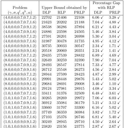
Comparison of Upper Bounds Table 1 gives the upper bounds obtained by DLP, RLP and PRLP. VCE and SAA do not provide upper bounds on the optimal expected profit and these solution methods are omitted in this table. The first column in Table 1 shows the problem characteristics. The second, third and fourth columns, respectively, give the upper bounds obtained by DLP, RLP and PRLP. The next two columns respectively give the percentage gap between the upper bounds obtained by RLP and DLP, and RLP and PRLP. The “X” in the columns emphasize that the gaps are all significant at the 95% level. The results in Table 1 indicate that RLP generates significantly tighter upper bounds than both DLP and PRLP. The average percentage gap between the upper bounds obtained by DLP and RLP is around 5%, while the average gap between the upper bounds obtained by PRLP and RLP is around 4%. While PRLP provides a slightly tighter upper bound than DLP, we can further tighten the upper
bound quite significantly by using RLP. This may justify the extra computational effort in simulating the show-ups in RLP as opposed to using just the expected number of show-ups in PRLP.
Comparison of Expected Total Profits Table 2 gives the expected total profits obtained by the five solution methods. The columns have the same interpretation as in Table 1 except that they compare the expected profits obtained by DLP, RLP, PRLP, VCE and SAA. The last four columns in Table 2 give the percentage gap between the expected profits obtained by RLP and the other benchmarks. We obtain the expected profits by simulating the bid price policies obtained by the different solution methods under multiple realizations of the demand and show-up random variables. We use common random numbers in our simulations; see Law and Kelton (2000). The last four columns in Table 2 include a “X” if RLP does better than the respective solution method at the 95% significance level, a “×” otherwise and a “⊙” if there does not exist a statistically significant difference between the two.
Comparing the expected profits in Table 2, we observe that RLP and SAA typically generate the highest profits followed by DLP, VCE and PRLP without a consistent ordering between the latter three solution methods. The performance gap between RLP and DLP is around 3% on average, but we observe performance gaps as high as 8%. RLP performs better than DLP in 23 out of the 24 test problems and the gaps are statistically significant in 21 test problems. We observe one instance where DLP performs better than RLP, but the performance gap is less than half a percent. RLP performs better than PRLP in all of the test problems and the average performance gap is around 6%. A similar observation holds when we compare RLP with VCE and the average performance gap between these two solution methods is around 5%. The profits generated by RLP and SAA are comparable with the average performance gap being around -0.19%. In 20 out of the 24 test problems, there is no statistically significant difference in the profits generated by RLP and SAA. SAA does better than RLP in three test problems, while RLP does better than SAA in one test problem. To our knowledge, SAA is one of the strongest methods to compute bid price policies for joint overbooking and capacity control problems and it is quite encouraging that the performance of RLP is comparable to that of SAA.
Despite the fact that the performance of RLP and SAA are quite close to each other, there are a number of reasons that may make RLP preferable to SAA from practical perspective. To begin with, RLP provides an upper bound on the optimal expected total profits while SAA does not. In fact, DLP is, to our knowledge, the only other computationally tractable method that can obtain upper bounds on the optimal expected total profits when overbooking is allowed. RLP significantly improves the upper bounds provided by DLP, yielding improvements up to about 8%. Tighter upper bounds on the optimal expected profits can be quite valuable when assessing the optimality gap of approximate control policies. Another attractive feature of RLP is that the implementation of SAA requires tuning a number of parameters such as the step size rule and the stopping criterion of the stochastic approximation algorithm, for which there are no hard and fast rules. The implementation of RLP tends to be easier as it involves only selecting the sample sizes K and L. While doing a reasonably exhaustive search over all step size rules and stopping criteria is virtually impossible, one can certainly test quite a few different choices ofK andLfor RLP and settle on a choice. It is also worthwhile to point out that RLP requires solving linear programs, minimizing the need for customized coding. Finally, an important
advantage of RLP over SAA is the running time. Table 3 compares the CPU seconds to solve RLP and SAA on networks with different numbers of spokes and booking horizons with different numbers of time periods. After a few setup runs, we settle on K = 25 and L = 200 in our implementation of RLP and run SAA for 5000 iterations. The left and right portions Table 3 respectively show the CPU seconds for different numbers of spokes in the airline network and different numbers of time periods in the booking horizon. All of the computational experiments are carried out on a desktop PC running Windows XP with Intel Core 2 Duo 3 GHz CPU and 4 GB RAM. We use CPLEX 11.2 to solve all the linear programs. The running times for RLP and SAA are generally comparable and are of the order of minutes. The running time of SAA is independent of the number of time periods since SAA works with an aggregate formulation, which requires only the total number of product requests but not the sequence in which the requests arrive over time. However, the running time of SAA can grow quite rapidly as the size of the airline network measured by the number of spokes increases. DLP, PRLP and VCE take at most a few seconds to solve and we do not provide their running times in Table 3, but the performance of these solution methods is not competitive to RLP or SAA.
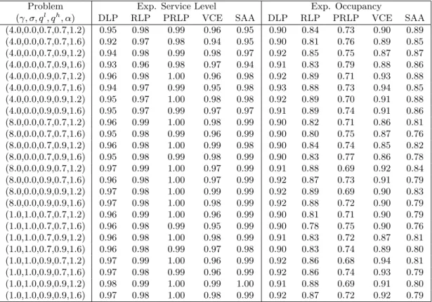
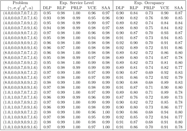
Comparison of Service Levels While the benchmark solution methods are all designed to maximize the expected profits, this may not necessarily be the only performance measure that is of interest to the airline. In Table 4, we compare the solution methods on two other dimensions, namely the service levels and the occupancy levels. The service level gives the fraction of the show-ups that are allowed boarding, while the occupancy level is the fraction of seats that are occupied when the flights depart. The first column in Table 4 shows the problem characteristics. The next five columns give the expected service levels achieved by DLP, RLP, PRLP, VCE and SAA respectively, while the last five columns give the corresponding occupancy levels.
We observe that PRLP has the highest service levels, followed closely by RLP and SAA. VCE and DLP tend to have slightly lower service levels associated with them. On the other hand, when we compare the occupancy levels, DLP and VCE tend to have the highest occupancy levels, followed by RLP and SAA. PRLP tends to have a significantly lower occupancy level than the remaining solution methods. The above observations suggest that PRLP tends to be conservative in accepting product requests. As a result, it is able to provide service to almost all of the reservations that show up. Its denied service cost tends to be low, but at the same time, its revenues also tend to be low because it accepts only a smaller number of product requests. The net effect is lower profits. On the other hand, DLP and VCE tend to be more aggressive in accepting product requests. As a result, their revenues and occupancy levels tend to be higher. However, they may have to deny boarding to a greater fraction of the reservations that show up, which leads to lower service levels. Therefore, although DLP and VCE obtain higher revenues, they also tend to have higher denied service costs, resulting in lower overall profits. RLP and SAA seem to achieve a good balance between the service and occupancy levels. The service and occupancy levels of RLP and SAA lie in between the other solution methods. They tend to be more selective, accepting fewer but higher-value product requests. Since they accept higher-value product requests, their revenues are comparable to DLP and VCE. On the other hand, since they accept fewer number of product requests, their denied service costs are comparable to PRLP. The net result is that their overall profits tend to be higher than DLP, VCE and PRLP.
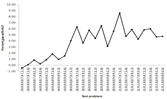
Qualitative Behavior of RLP Figure 2 gives a feel for the problem parameters than boost the performance of RLP relative to DLP. The horizontal axis gives the problem parameters. The test problems are so arranged that two consecutive problems differ only in the tightness of the leg capacities. Blocks of eight consecutive test problems have the same penalty costs of denied boarding and the penalty costs get larger as we move from left to right. The figure indicates that the performance gap between RLP and DLP generally increases as leg capacities get tighter. We also see that the performance gap between RLP and DLP increases as the penalty costs of denied boarding increases. Problems with tight leg capacities and large penalty costs tend to be more challenging to solve because the consequences of accepting an “incorrect” product request tend to be more severe. It is encouraging that RLP seems to be an attractive alternative to DLP in such settings.
Figure 3 shows how the upper bound obtained by RLP changes with the number of demand simulations K and the number of show-up simulations L. We see that RLP is fairly robust to the number of demand and show-up simulations and we obtain stable results for K ≥25 and L≥100. To be on the safe side, we use K= 25 and L= 200 in our computational experiments.
6.3 Computational Results for the Network with Two Hubs
Computational Setup We have a network with two hubs serving a total of N spokes. The first half of the spokes are connected to the first hub and the second half of the spokes are connected to the second hub. Each spoke has one flight to and one flight from the hub that it is connected to. In addition, we have one flight from the first hub to the second and another flight in the reverse direction, so that the total number of flights is 2N + 2. Figure 4 shows the structure of the network for the case where
N = 8. The hub and each of the spokes serve as both origins and destinations. We have a high-fare and a low-fare product connecting each origin-destination pair. We randomly sample from the set of all origin-destination pairs so that the total number of products is around 150. The remaining problem parameters are set in the same manner as for the test problems with a single hub. In particular, a high-fare product is four times as expensive as the corresponding low-fare product for each itinerary.
We label our test problems by (γ, σ, ql, qh, α), where the parameters have the same interpretation as in the test problems with a single hub. We have (γ, σ) ∈ {(4,0),(8,0),(1,1)}, ql ∈ {0.7,0.9},
qh ∈ {0.7,0.9}and α∈ {1.2,1.6}, which provides us with 24 test problems. In all of our test problems, we have 8 spokes and 360 time periods in the booking horizon.
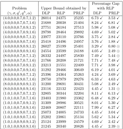
Comparison of Upper Bounds, Expected Total Profits and Service Levels Table 5 gives the upper bounds obtained by DLP, RLP and PRLP. The columns in this table have the same interpretation as in Table 1. The results in Table 5 indicate that RLP continues to generate significantly tighter upper bounds than DLP and PRLP. The average percentage gap between the upper bounds obtained by DLP and RLP is around 6%, while that between PRLP and RLP is around 4%.
Table 6 gives the expected total profits obtained by the five solution methods. The columns in this table have the same interpretation as in Table 2. The results generally follow the same pattern
as for the test problems with a single hub. RLP and SAA generate the highest profits followed by DLP, VCE and PRLP. The average performance gap between RLP and DLP is around 4%. The gaps are statistically significant in 20 out of the 24 test problems. In the remaining four test problems, the performance gaps between RLP and DLP are not statistically significant. The average performance gap between RLP and PRLP is around 9%, while that between RLP and VCE is around 6%. The gaps are statistically significant in all of the test problems. The profits generated by RLP and SAA are very close. The average performance gap between RLP and SAA is around -0.15%. In 18 out of the 24 test problems, there is no statistically significant gap in the profits generated by RLP and SAA. SAA does better than RLP in four test problems, while RLP does better than SAA in two test problems.
Finally, Table 7 gives the service and occupancy levels achieved by the five solution methods. The average service levels of DLP, RLP, PRLP, VCE and SAA are 0.96, 0.98, 1, 0.97 and 0.99 respectively. On the other hand, the average occupancy levels of DLP, RLP, PRLP, VCE and SAA are 0.9, 0.84, 0.72, 0.89 and 0.81 respectively. We again observe that RLP and SAA seem to achieve a good balance between the service and occupancy levels.
7 Conclusions
In this paper, we developed a randomized linear program to jointly make the capacity control and overbooking decisions on an airline network. Our solution approach builds on a linear programming based formulation of the network revenue management problem, where we make the capacity control and overbooking decisions after observing a realization of the demands for the products. We establish that this formulation yields a tighter upper bound on the optimal expected total profit than the deterministic linear program. We show that the upper bound provided by the deterministic linear program is asymptotically tight, which implies that the upper bound provided by the randomized linear program is also tight. Furthermore, our proof technique for this result generates a policy from the deterministic linear program whose expected total profit is asymptotically optimal.
As it is difficult to compute the expectation of the objective value of the randomized linear program analytically, in our practical implementation, we use samples of the demand and show-ups to approximate the expected values. We solve the resulting sample average approximation and use the optimal values of the dual variables associated with the flight leg capacity constraints to get a bid price control policy. Our computational experiments indicate that our approach can generate significantly tighter upper bounds and higher profits compared to numerous standard benchmark methods.
A Appendix: Obtaining a subgradient of zRLP
In this section, we show that zRLP is a concave function of the capacities of the flight legs by showing that it has a subgradient. Furthermore, the expression that we obtain for the subgradient of zRLP motivates the bid price policy that we derive from the randomized linear program. To emphasize the dependence on the flight leg capacitiesc={ci:∀i}, we writezRLP andzRLP(d) respectively aszRLP(c)
andzRLP(d, c) throughout. Noting thatStakes on only finitely many values and−min{x}= max{−x}, we can write problem (16)-(17) equivalently as
zRLP(d, c) = max n ∑ j=1 τ ∑ t=1 fjyjt− ∑ s∈{0,1}nτ Pr{S =s} n ∑ j=1 τ ∑ t=1 θjwjts (35) subject to n ∑ j=1 τ ∑ t=1 aij[sjtyjt−wsjt]≤ci ∀i, s (36) 0≤wsjt ≤sjtyjt ∀j, t, s (37) 0≤yjt ≤djt ∀j, t, (38)
where Pr{S =s} is the probability thatS takes on a value s∈ {0,1}nτ and we use wsjt to denote the number of product j reservations that are denied boarding when S =s. Letting ρds(c) ={ρdsi (c) :∀i}
denote the optimal values of the dual variables corresponding to constraints (36), it follows from the linear programming duality theory that zRLP(d,ˆc)≤zRLP(d, c) +
∑m i=1 ∑ s∈{0,1}nτρids(c)[ˆci−ci]. Since zRLP(c) =E{zRLP(d, c)}= ∑ d∈{0,1}nτPr{D=d}zRLP(d, c), we obtain zRLP(ˆc)≤zRLP(c) + m ∑ i=1 [ˆci−ci] ∑ d∈{0,1}nτ Pr{D=d} ∑ s∈{0,1}nτ ρdsi (c).
This implies that, if we let ρi(c) = ∑ d∈{0,1}nτPr(D =d) ( ∑ s∈{0,1}nτ ρdsi (c) ) , then ρ(c) = {ρi(c) : ∀i} is a subgradient of zRLP(c) with respect to c. In our Monte Carlo estimate of this subgradient, we use
ρi = ∑K
k=1K1 ∑L
l=1ρkli as an estimate of ρi(c), whereK and L are respectively the number of demand and show-up simulations. This is precisely the bid price that we use in the decision rule in (24).
B Appendix: Proof of Proposition 5 and Asymptotic Tightness
In this section, we give a proof for Proposition 5. In doing so, we also derive a policy from the deterministic linear program whose performance is asymptotically optimal as the problem size, measured by κ, gets large. Therefore, not only the upper bound on the optimal expected total profit provided by the deterministic linear program is asymptotically tight, we can also derive a policy from the deterministic linear program whose performance is asymptotically optimal.
Our first observation is that if (ˆy,wˆ) is an optimal solution to problem (6)-(10), then (ˆyκ,wˆκ) with ˆyκjt = ˆyj⌈t/κ⌉ and ˆwjtκ = ˆwj⌈t/κ⌉ is an optimal solution to problem (25)-(29). Thus, noting that the optimal objective values of problems (6)-(10) and (25)-(29) are respectively denoted byzDLP andzDLPκ , it follows that zκDLP =κ zDLP.
Now, we consider the following policy π for problem Pκ. We solve problem (25)-(29) to obtain the optimal solution (ˆyκ,wˆκ). For accept and reject decisions, we accept a request for product j at time period t with probability ˆyκ
jt/pκjt. At the departure time, if a reservation for product j made at time period t shows up, then we allow it to board with probability 1−wˆκjt/(qκjtyˆjtκ), provided there is sufficient remaining capacity on the flight legs used by that product. That is, we first flip a coin to