331
COMMENT AND DEBATE
Social class differences in early cognitive development
(Received April 2015 Revised June 2015) http:// dx.doi.org/10.14301/llcs.v6i3.361
John Bynner
Few pieces of recent longitudinal research have had as much influence in United Kingdom policy circles as Leon Feinstein’s analysis of 1970 birth cohort study data (reported in 2003) on cognitive development assessed at ages 22 months, 42 months five years and ten years. Breakdown by social class of the test performance data demonstrated that infants of superior cognitive ability in the first assessment from working class backgrounds showed relative decline with age in test performance compared with their middle class counterparts, who while starting from an inferior position, subsequently overtook the working class group. The findings were embodied in what became a famous graph showing this crossover and consequent reversal of predicted life chances. They pointed to substantial obstacles to social mobility and were an important factor in the policy response of major pre-‐school educational interventions such as the Sure Start programme introduced by the Labour Government to reverse the trend, which attracted support from across the political spectrum.
Subsequent re-‐analysis by John Jerrim and Anna Vignoles challenged the existence of the crossover as a statistical artefact attributing it to the well-‐known phenomenon of ‘regression to the mean’. The consequence was a cooling off of support for the intervention policy directed at strengthening working class children’s early cognitive performance. This shift included termination of the Sure Start programme by the new Coalition Government (Conservative and Liberal Democrat) that took office in 2010. Subsequent research has qualified the picture further raising issues on a number of methodological and substantive fronts – especially the need to give more attention to measurement error in such work and for a more nuanced interpretation of such longitudinal research results. Social class disadvantage in cognitive development is well established but the relative loss of competence developmentally needs to be treated with caution.
In an opening paper Leon Feinstein reviews the methodological criticism of his original research. The points he raises are then debated in commentaries by John Jerrim and Anna Vignoles, Harvey Goldstein and Robert French, Elizabeth Washbrook and RaeHyuck Lee and Ruth Lupton. Leon Feinstein's response to these will be published in the next issue of the journal.
Opening paper by
Leon Feinstein
Early Intervention Foundation, UK
Social class differences in early cognitive development and regression to the mean
Introduction
In April 2011 the then new Coalition Government published its social mobility strategy (HM Government, 2011). As a minor reference within the overall document, figure 2 of Feinstein (2003) was reproduced on page eight as a reference to the
claim that “Bright children from poorer families tend to fall back relative to more advantaged peers who have not performed as well.”
that:
I am very worried that this graph is being used to shape policy when in fact many statisticians will instantly see that it simply replicates a statistical trap or artefact called ‘regression toward the mean’. The apparently shocking pattern of results in the graph is simply what statisticians would expect when you measure extremes of performance in two populations of differing ability. The Feinstein graph is constructed... with undue emphasis on extreme results.
Simultaneously, Jerrim and Vignoles (2011), published a paper on the “use (and misuse) of statistics,” undertaking a series of simulations and new analyses based on a model assuming “true abilities” with pre-‐determined social class mean gaps, which shows that under reasonable assumptions the pattern in the chart could result from regression to the mean.
The 1970 Cohort Study is no longer such a significant source of information on the degree of British inequality in contemporary childhood. We have now much larger and more recent studies such as the Millennium Cohort Study, the first major, public United Kingdom (UK) birth cohort study since the 1970 Cohort and the Life Study at University College London (UCL) with an intended sample of 100,000 babies and a wide range of developmental, health epigenetic and neuro-‐ scientific observations.
But the 1970 Cohort data in general are still of considerable interest and many of those who may have quoted the graph in the past may have been disappointed to learn that they had been so badly misled so I am grateful to the editors of this journal for the opportunity to respond to the critique and to raise a handful of questions for further debate. As the quotations above make clear, there is a wider debate both in learned journals and on the pages in the national newspapers. They do not operate by the same rules. I am grateful to the
editors for inviting this paper in a special comment and debate section of the journal that is also about the relationship between research, policy and practice.
Some in the policy world have used the graph without understanding it, though it is perhaps hard to see this an issue specific solely to this chart. Some of those who have used it have understood its weaknesses but found it informative, some have had no idea and are horrified it is all so complicated. Few will have much mind to it. Without wishing to reinstate the graph as a “killer chart”2 I would like, in this paper, to correct some of the mis-‐ representations that have been suggested and suggest some issues for further discussion.
The graph was based on a relatively small sample from a time and place that is, with due respect to its members, now distant. The Britain of today is transformed in terms of ethnicity and the way inequality is experienced. Much larger datasets are available with much larger samples and more consistent measurement across a broader range of aspects of cognitive development. New methodologies are available. So my argument is not that anyone should return to this chart as the way to model and measure the interaction of a distal measure like class and tests of cognitive ability through childhood, but that there are a range of ways of modelling these data, recognising the importance of the measures used, the age at which children are tested, how different models lead to different tests of this social level interaction and how this plays out in different times and places. I set out below the basic facts of the graph and then discuss in more detail what I think the graph means and raise some questions about meaning and inference, in particular with regard to the definition of true ability and the difference between average, macro-‐social phenomena and the lives of individuals. The first section sets out first the charts and then their source. The second section describes some of the challenges for inference that it has raised. The third section concludes with reference to these themes.
333
The chart
Figure 1: Average rank of test scores at 22, 42, 60 & 120 months, by socioeconomic status
(SES) of parents
70
65
60
55
50
45
40
35
30
22 28 34 40 46 52 58 64 70 76 82 88 94 100 106 112 118
months
Figure 2: Average rank of test scores at 22, 42, 60 & 120 months, by SES of parents and
early rank position
100
90
80 High SES, high Q at 22m (n=105)
70
60
50
40
High SES, low Q at 22m (n=55)
Low SES, High Q at 22m (n=36) 30
20 Low SES, low Q at 22 m (n=54)
10
0
22 28 34 40 46 52 58 64 70 76 82 88 94 100 106 112 118
months
High SES
Medium SES
Low SES
Av
e
ra
g
e
po
si
tion
in
di
st
rib
ut
ion
Av
e
ra
g
e
po
si
tion
in
di
st
rib
ut
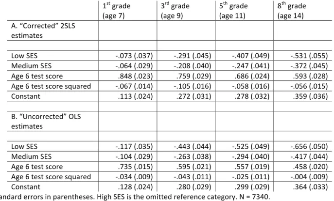
Figure 1 in Feinstein (2003) reports the mean relative positions of children in the 1970 British Cohort Study from different social class groups in age appropriate and hence very different tests of cognitive development at four ages in early and middle childhood (ages 22 months, 42 months, five years and ten years). The explicit rationale of the paper was to test the extent to which average gaps in cognitive development between children from different types of family background were evident before children started school. The difficulty of testing this and of comparing gaps at different ages seemed to centre on the difficulty of finding comparable tests through the complex qualitative developmental changes that occur in early child development. The innovation of the paper was in finding a coherent way to simplify and address the problem. It made possible a cursory, uni-‐ dimensional study of development at the level of average groups of children.
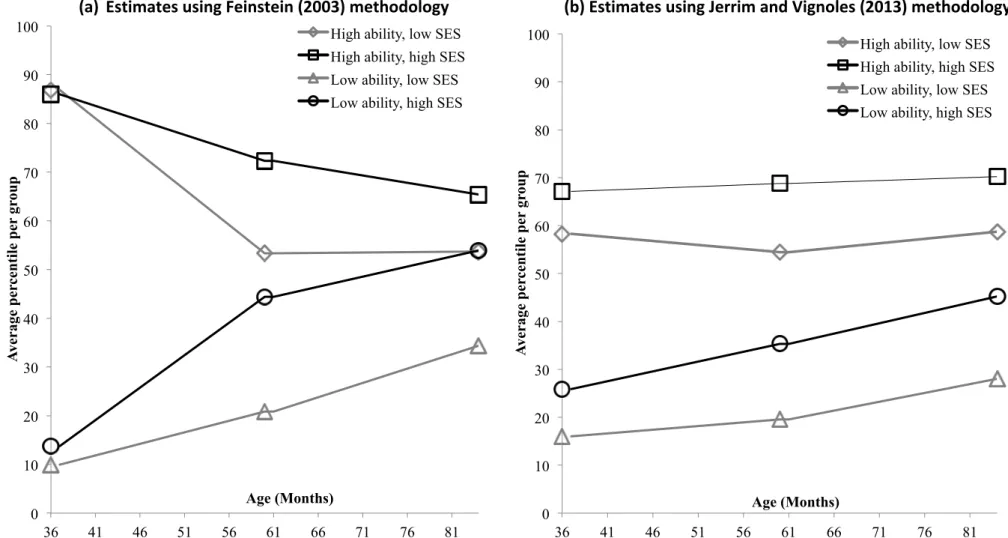
Figure 2 indicates some of the interaction between family background and early ability scores, at particular points of the distribution of early scores.
The main rationale of the paper and of initial discussion of it was of the finding of early socioeconomic status (SES) gaps in figure 1. Figure 2 subsequently became used by me and others in public debate, showing that the children from high SES backgrounds who scored poorly on the age 22 month tests had a higher mean score at 10 years than the low SES children who scored well in the early tests. The shift in relative mean position occurs between the age of five and ten. This always seemed to me remarkable, though recognising that it may be due in untested proportions to measurement error, context, gene*environment interactions, gene*environment correlations and cultural bias. As I said at the time, the graph does not and cannot resolve the question of explanation but it does describe a very common pattern in UK data.
Methods and measurement
SampleThe 1970 Cohort Study was a representative sample based on children born in the first week of April 1970 undertaken initially by the Department of Child Health at Bristol University and taken on to adulthood by the International Centre for Child Studies, City University and then the Institute of Education. Data was collected from members of the
cohort studies and from members of their households, through a range of tests and interviews at different ages, as well as through interviews with teachers and medical officers.
The full sample comprising 17,196 children were studied at birth, of whom 13,135 were picked up at age five years and 13,871 at ten years. For the 2003 paper, data were also drawn from the 22 month and 42 month sub-‐samples of the study. These studies initially comprised 2,457 individuals, of which half were selected from the full sample because at risk of foetal malnutrition and half as a random control group. Attrition and non-‐ response provides a sample of 1,292 children providing test score data and a measure of SES at ages 22 months, 42 months, five years and ten years. This degree of sample loss represents a tremendous achievement by the study team. It is not unproblematic if attrition is non-‐random such that the remaining sample is no longer typical of the population it is intended to represent. The kind of non-‐randomness required to cause bias to the general indications of figure 1 and 2 would be one in which children most likely to have been omitted were ones for whom on average the relationship between SES and the development of test scores was different than for the included children.
There is no evidence of this. The paper did have an eye to the differences between children in the control group and those who were selected for the sub-‐sample because of a distal concern about foetal development. Both issues of sample selection and attrition merit further work. If the paper were to be published today referees would require a greater focus on the handling of missing data than was the case before Little and Rubin (2002) and others had created software and approaches to handling missingness and a greater appreciation of its importance.
Socioeconomic status (SES)
335
SES was used for each child, rather than allowing it to change through childhood as family circumstances evolved. The birth measure was used where this was available. Second, the measure was an aggregation of the SES of the male and female adults in the household, in most cases the biological parents. The majority of the mothers of the children in the 1970 Cohort were not working and for these children SES was categorised on the basis of the father’s occupation. Where both parents were working and had occupations in different SES groups, high or low SES dominated in the categorisation, such that a child in a household with a high SES father and middle SES mother would be categorised as high SES and vice versa. The very small number of high/lows were categorised as middle.
The intention was to create a simple indicator of occupational skills and access to earnings and status in the economy and society of the day. The broad pattern of results was found to be very similar if groups were constructed on the basis of parents’ education levels (Feinstein 2003). The intention was not to indicate that these groupings reflected common genetic inheritances or to indicate anything causal about social class nor to test hypotheses about the nature of social class. Other ways of classifying the children based on different ways of reflecting aspects of family backgrounds such as the distinct contributions of work situation and market situation (see e.g. Erikson 1984) or different ways of reflecting mothers’ and fathers’ contributions to each would have been possible and equally of interest. These are broad averages based on the available data on the occupation of parents.
Cognitive performance
Comparing measures of cognitive performance at different ages in childhood is made particularly difficult by the qualitative shifts in development that transform the meaning of cognitive capability as children mature. At each age in these data a different set of tests are taken by the children because the tests span the period from early to middle childhood through which considerable shifts in the meaning, nature and measurable manifestation of cognitive development takes place. Piaget (1952), for example distinguishes the sensorimotor stage, from birth to age two in which infants seek and find knowledge through sensory experiences and manipulation of objects; the preoperational stage, from age two to about age
seven in which pretending and play are evidently essential to learning; and the concrete operational stage, from age seven to 11 in which logic becomes more routine if at times rigidly applied. In Piaget there is also a formal operational stage, which begins in adolescence and spans into adulthood with an increase in logic, the ability to use deductive reasoning, and an understanding of abstract ideas. There are of course many other models of the nature of developmental change in this period but it is not disputed that very fundamental qualitative change in behaviour and capability occurs through early childhood.
The 22 months tests comprised cube stacking, measures of personal development, measures of language use and a drawing task. The information was collected by a health visitor recruited by the Department of Child Health at the University of Bristol during a visit to the home or other residence of the sample children3. The personal development measures were a set of requests from the health visitor to the child such as to point to her nose or her eyes. The cube-‐stacking test was designed as a test of motor ability, a precursor of later capabilities such as intelligence as well as of physical dexterity. The measures of language use concerned the child’s ability reported by the mother to say “ma-‐ma” and “da-‐da” and associate the words with the appropriate persons.
The measures as a whole were less well standardised than measures available in the newer UK cohort studies (Chamberlain and Davey, 1976), but merit further study. At age ten years the tests were of maths and reading and the British ability scale test of IQ.
Therefore these measures reflect the transition from early public language use as a 22-‐month-‐old child responds to the request from a health visitor to point to her nose to the experience of the age ten child sitting a maths test in a classroom. The relationship between the different features of cognitive and non-‐cognitive development that lead from the 22 month child pointing to her nose when asked to and the girl sitting the exam are only partially understood but it is clear that there is no simple linear relationship between specific domains of development in early childhood and equivalent domains in adolescence or adulthood.
table) and “speaking” (correctly naming pictures such as of a car) and a copying designs test, all conducted by trained researchers or health visitors in the home. At age five years there was a test of vocabulary, a copying designs test and a human figure-‐drawing test (Feinstein, 2003). The age 42 month speaking and counting tests are equal in the prediction of the age ten maths and reading scores with little domain continuity spanning across early to middle childhood (Feinstein, 2003). Not surprising as the tasks all involve elements of language, communication, motor skills and attention, amongst other capabilities.
More and better modelling of this issue is possible now in multiple datasets, not least the Avon Longitudinal Study of Parents and Children which has annual measurement across a much better set of measures of cognitive and other development than were possible in the 1970 Cohort Study.
It is important to emphasise that in order to derive the best possible signal from the available data, the measure used in the graph at each age is not any single test but rather the ordinal position of the children at each age in a weighted average of the scores available at that age. The particular form of weighting is the first principal component, chosen to maximise the variance in the weighted index. Particular tests count higher in the weighting if they add more unique information than other tests. The results are robust to the use of other weighting schema such as regression weights taken from regressing the age ten tests on the earlier tests. Therefore, although the measures used change through development the dependent variable itself is always the relative achievement of the sample children at each age in the age appropriate measures of cognitive development available in the 1970 Cohort Study.
The implications of this are that the dependent variable is ordinal position and has meaning only in this relative sense. It does not measure achievement on any specific test but is an estimate of relative cognitive capability in the available age-‐ appropriate measures. It is therefore different to the repeat measures test that Jerrim and Vignoles (2013) use in their analysis of the Millennium Cohort Study.
Descriptive findings
Figure 1 reports the average (mean) relative positions of children classified by the three-‐fold
categorisation of social class on the single measure of relative ability drawn from the range of age appropriate but different tests at each of the four ages.
Figure 2 reports the mean scores of children from different social class groups at the four ages. Critically, it classified children according to their scores on the first set of tests at age 22 months and considers also the mean scores for children depending on their rank in the early scores.
The early scores are particularly unstable. As I show in the original paper they contain sufficient real information about early development to predict final educational qualifications achieved but the correlation is only just statistically significant and weak. Therefore, as I also show in the original paper, it is not surprising that children’s scores subsequently move around a great deal.
Subsequent discussion has focussed on the meaningfulness of the crossover in figure 2, regression to the mean, the appropriateness of classifying children to ability groups at 22 months and the focus on arbitrary quartile groups.
Inference and regression to the mean
When the graph was first presented at an econometrics seminar at UCL issues were raised about measurement error and causality. Then and since there have been debates about regression to the mean, a notion whose original use was by Galton (1886) who discussed the issue in terms of the tendency of the individual deviation from the mean in height to be larger in one generation than the next, so that tall parents will tend to have slightly less tall children. The degree of randomness in a variable through measurement error or chance will mean that the deviation from the mean in one period is that much less likely to be replicated in the next.
In this instance regression to the mean refers in part to the statistical property by which because of misclassification bias in the early groupings, those who appeared to do well early on will have a tendency to lower scores in subsequent tests. Conversely, those who score badly early on will have a tendency to better scores. This was shown by Tu and Law (2010) to be a fatal problem for interpretation of the chart as the outcomes for those from different social class groups with different “true” ability.
337
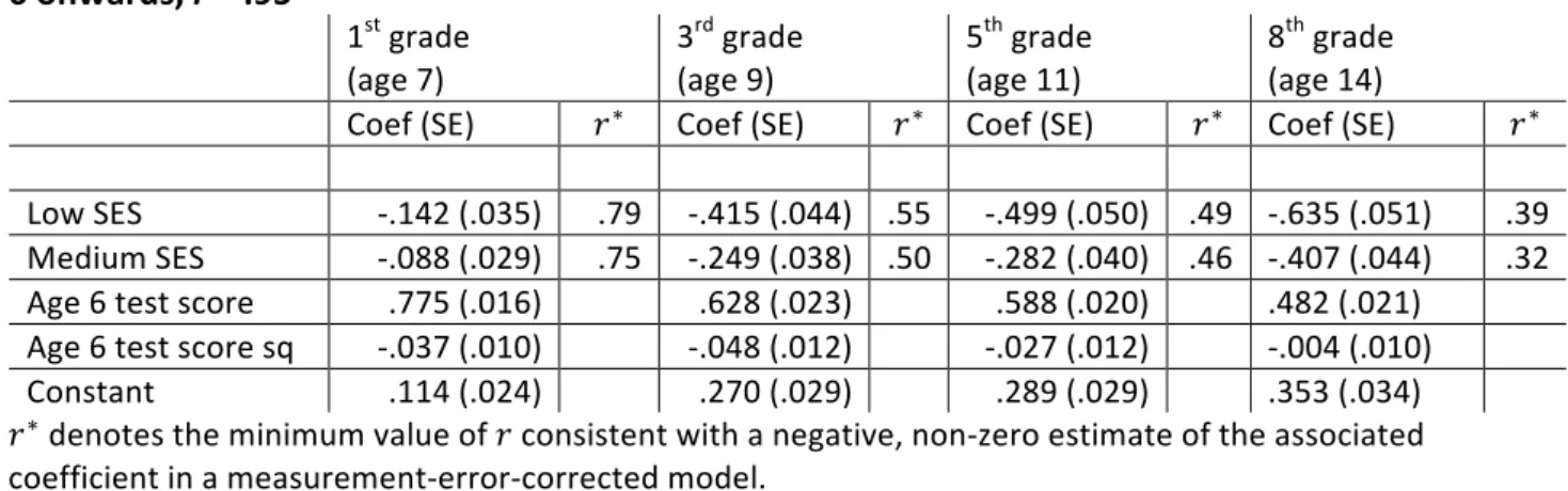
Vignoles (2011; 2013) have shown how regression to the mean plays out in the kind of data shown in the chart and also used the phrase in other ways. Using simulations, they show that the pattern observed in the chart can be substantially reproduced as the result of regression to the mean of various kinds, including both error in measurement and hence classification to high and low groups and differences in what is tested at different ages.
They reference Nick Clegg’s use of the phrasing that: “By the age of five, bright children from poorer backgrounds have been overtaken by less bright children from richer ones — and from this point on, the gaps tend to widen still further.” Jerrim and Vignoles wanted to correct the misapprehension that the graph shows that bright working class children in mid-‐childhood will necessarily fall behind dim middle class children in middle childhood. This misapprehension would be based on the presumptions that: the graph represents a necessary feature of the development of all individuals rather than representing average phenomena; and that it is meaningful and technically possible to identify stable cognitive capabilities at 22 months such that “bright” and “dim” children can meaningfully be identified and classified as such based on tests at 22 months. Yet, it is not necessary to believe that the groupings are stable, innate or fixed to find the data in figure 2 interesting. The graph shows what happens to the average test scores of different clusters of children in an interaction between an indicator of family origin and average measures of cognitive development, starting very early in childhood. Low social economic status (SES) children in the UK tended (and still tend) on average to fall back relative to middle class children, whatever the early levels of measured ability. Read (2003) is wrong that the shift between 22 and 42 months was taken by policy makers to be substantive.1 Much of the chart’s role in public debate was as a proxy for a much wider body of research, including more recent analysis of the National Pupil Database and other more recent cohort studies showing how at every stage of education, low income children tend to progress at a slower rate on average than those on higher incomes (Kingdon and Cassen, 2007; Goodman and Gregg, 2010; Magnuson, Waldfogel and Washbrook, 2012). The broad fact is not disputed that the
relative access of parents to wealth, income and educational knowledge on average tend to be replicated across generations, in the UK, now and in the past.
It is regrettable that Feinstein (2003) did not include more consideration of the reliabilities of the measures used because differences in reliability at different ages are likely to be responsible for a considerable but unquantified part of the observed pattern of results as children mature. If reliability of measurement increases with age then one might expect the fanning observed in figure 1 and the resulting pattern of figure 2. It is also important that the age ten tests may be more discriminating as tests of cognitive development than the age five tests.
The intention in Feinstein (2003) was explicitly descriptive, aiming to offer a sense of scale of the emergence of the gaps in average scores by children classified in very broad groupings in a very raw and single index of cognitive development. Measurement error was not dealt with. The aim was to present the actual data, of the kind that is used to test children and award them grades and qualifications, suffering as this does from measurement error, rather than to present corrected trajectories based on modelling assumptions.
The change between ages five and ten years
Jerrim and Vignoles show that under reasonable, though not proven, assumptions the misclassification bias in the average score washes out after the second point of measurement. Therefore, the change in relative position between age five and ten years may be substantive. They note it may be due to a difference in the underlying tests, and suggest therefore this should also be seen as a form of regression to the mean.However, there are other sorts of possible measurement error that may well be persistent across ages, depending on what is meant by true ability. Some have argued (Gillborn & Youdell, 2000) from a more sociological perspective that low SES children will tend to under-‐perform in tests of cognitive capability because the tests reflect codes, expectations and structures of power that are themselves class-‐based.
Perhaps authors in this series might comment on the likelihood and implications of the assumption of zero correlation in measurement error across ages. I certainly agree that the difference in the underlying tests is important, but labelling this regression to the mean in a public debate seems to me to confuse the error resulting from misclassification bias in the early tests with the idea of a genetic basis to social class groups. Although this latter shift could technically be described as “regression to the mean,” it is of a very different sort to that of the first kind, and is not adequately explained as necessarily a statistical phenomenon. This is an issue on which further clarification would be useful. Although concerned with measurement, I see the data in figure 2 as evidence that children from working class families in the 1970 Cohort Study who not only scored well at 22 months on fairly raw tests of cognitive capability, but continued on average to do so at ages 42 months and five years, did not on average translate this ability into school success at age ten at anything like the rate of children in middle and upper class families. The shift from more general features of cognitive development at age five to more scholastic tests of reading and maths is important. Working class children in the 1970s appear to have tended to do worse on average on the age ten scholastic tests than they did on the more general age five tests. Some may argue this is because the age ten tests are better measures of true ability and so better indicate the true abilities of children from the different social class groups. My interpretation is more that the working class children tended to translate their earlier capabilities into success in scholastic test scores less well than did their middle class peers. As has been said many times the graph does not resolve this question.
By age ten it is meaningful and possible to conduct long tests of what children have learned in school. The age five tests are much more generic tests of cognitive capability. So it is informative that
whereas middle class children who scored well on the age five copying test tended to score well in later tests, working class children did so to much less of an extent. It may be, as some appear to assume, that working class children who did well on the copying test just got lucky. It seems more likely to me that they just didn’t achieve their potential in the later tests. The data do not distinguish between these interpretations.
True ability
There are both statistical and political debates being had and much as statisticians might like the rules of political debate to be reduced to the conventions of statistical debate, this is unlikely to happen. The graph has caused confusion in some quarters because of the difficulty of translating accurate and reasonable interpretations for policy audiences. This has also been difficult for Jerrim and Vignoles whose critique of the false interpretation of the chart has been taken by some as proof that social mobility is inevitable (Saunders, 2011 and Guardian 14 April, 2011 “Government social mobility expert under attack.”). In other work Jerrim, Vignoles, Lingam and Friend (2013) show the huge gap between the evidence from structural genetics regarding the heritability of intelligence and that from any biological analysis of actual genetic data in explanation of the social class attainment gap. As discussed further below, it is important in the political debate that the Jerrim and Vignoles model is not taken as proof of its own assumptions, that low SES children are innately less cognitively capable, based on confusion about the meaning of “true ability” in their model. The notion of true ability they use is a statistical convenience, not the suggestion that science or social science has shown in any way that the latent ability gap at each age is in any way innate.
339
but it does not concord with a more usual, popular understanding of the notion of true ability, it is a statistical definition.A second key assumption of their model is that at all ages and moments of development the true component of their variable is socially stratified, that is to say reflective of the degree of wider structural inequality such that the 22 month differences in rank contain and reflect SES differences. They assume that it is a feature of true ability, as well as of test scores. This follows from their implicit definition of true ability as the latent construct at the time of the test, not from presuming that it is a fixed entity, as the Jerrim Vignoles model allows true ability to vary over time. Furthermore, Jerrim and Vignoles do not assume, as does Saunders (2010; 2011) that a social class gap in true ability is a necessary feature of society, occurring necessarily in all social aggregates in all times and places. However, their use of the phrase “true ability” in their statistical modelling does appear to have been taken by some to imply that their model showed that there are stable, biological foundations to the social class attainment gap. Crucially, Jerrim and Vignoles (2011), add to this the hypothesis that the degree of misclassification bias will vary by SES. Because low SES children are drawn from a group with a lower average score, children drawn from the low SES group who score well early on are more likely to have had, on their terms, over-‐estimated ability than the similarly scoring high SES children. They go on to say “Low SES children who get defined as high ability have probably had a particularly large random positive error (i.e. a lot of luck) during the initial test.” This is intended to be a statistical observation but we all need to be cautious in how we phrase attempts to explain statistical assumptions by making statements about people.
People, averages and qualitative change
Those I spoke to about the chart understood that it pertains to average rather than individual phenomena and so is an indicator of society and development in general not individual children. That said, I do particularly regret not being much clearer in public use of the study findings that the data in the two charts are averages. They may not describe the trajectories of any individual children. They are representative of a feature of development in general at the social level not of specific individuals.that changes qualitatively through the periods modelled. This is implied by the use of the lines alongside the data points of figure 2, which infuriated many, but it is important not to take this too literally as anything other than the changes in the average scores, that bear a distant relationship to the individual scores and are even more distant from the multi-‐ dimensional and complex development of the individual children. In recognising this, other models might treat these measures in very different ways.
The implication of a literal reading of figure 2 or of the Jerrim and Vignoles correction is that at each age it is unproblematic to compare children in terms of their true ability and stack them up in unique ranks of relative achieved uni-‐dimensional intelligence. Even at 22 months, their model assumes that the only barrier to achieving this is the technical difficulty of measuring these true ranks. Error results not just from poor measurement but also from the deviation of the “true” distribution of the underlying latent variable from the linearity assumption in the index. So it remains important not to overstate the resulting precision. In their corrections for regression to the mean Crawford, Macmillan and Vignoles (2014) are very careful to label this “high early performance,” to distinguish it from anything that might be thought innate, whatever the researchers’ intentions. These data in corrected form show a general tendency at a time and a place and between the ages assessed using the specific metrics available, not a fundamental and fixed truth about human beings.
There are a number of different explanations of the facts about cognitive development and social class in the UK. It is conceptually possible that the pattern between 42 months and age ten in figure 2 indicates how capability and context interact to influence outcomes for the children in the 1970 study and hence in general in England, Wales and Scotland in the 1970s. It is also conceptually possible that the pattern is entirely the result of regression to the mean in a very strong sense; that the high scoring working class children were just a group with low true ability with continued luck who eventually got found out as test scores got more accurate. It is true that the data do not discriminate easily between these interpretations. We are left with theory and the wider science to attempt to distinguish them.
Conclusion
The graph shows that children from working class backgrounds in the 1970 cohort with good very early signs of cognitive development were less likely to translate these early signals into good later scores than children from middle class backgrounds. From this graph and many other sources was drawn the line in the strategy: “Bright children from poorer families tend to fall back relative to more advantaged peers who have not performed as well.” I wouldn’t myself have used the phrase “bright children” but nothing in the Jerrim and Vignoles (2011, 2013) or Read (2003) critiques disprove the statement, as they themselves pointed out (The Guardian 28 April, 2011).
David Willetts MP, at the time Minister for Higher Education in the Department of Business Innovation and Science said subsequently:
Sometimes over-‐reliance on one specific piece of evidence can leave you vulnerable. I remember being influenced by Leon Feinstein’s very interesting paper for Economica in 2003 called Inequality in the Early Cognitive Development of British Children. He showed that bright poor kids fell behind rich dim kids by the age of 7. I served on Nick Clegg’s social mobility group and recommended this powerful evidence to him and he too was impressed and cited it. But Leon’s work was challenged by other academics because it was affected by reversion to the mean. The result was that the Guardian ran a piece that the Coalition’s social mobility strategy was undermined because the research on which it rested had been disproved. That is not, of course, a reason for giving up on evidence-‐based policy: but it is a reminder of how careful we have to be in using it.
341
bright working class ones. To be clear the crossover in this form is an artefact of the transparent way figure 2 was constructed and a corollary of figure 1. The point that was important for policy and was referenced in the 2010 Social Mobility Strategy was that throughout childhood in the UK children from low SES homes tend on average to fall back in school achievement relative to children from higher SES backgrounds.
The observed pattern between 22 and 42 months has always been understood by me and those with whom I have discussed the graph as mainly a statistical artefact resulting from measurement error. It has also been, in my experience, well understood that you cannot accurately or meaningfully fix children at 22 months on a scale of absolute and fixed ranks of ability. It would be wrong to define children as “bright” or “dim” on the basis of a set of early tests of cognitive development. Indeed, part of the early interest in the paper was because of the instability it showed in early signals of ability.
In an attempt at explaining the data (Feinstein 2003b, p30) I wrote, “so early scores do matter but so does social class after early childhood. The lesson for policy makers is clear. There is mobility (as one would expect) after 22 or 42 months, but upward mobility is mainly for high or medium SES children. Low SES children do not, on average, overcome the hurdle of lower initial attainment, combined with continued low input. Furthermore, social inequalities appear to dominate the apparent early positive signs of academic ability for most of those low SES children who do well early on.”
Some would like to argue this is just an inevitable fact of heredity (Lynn, 2011; Saunders 2011). Some have wanted to claim that these patterns of inequality in development demonstrate underlying genetic continuities such that inequality is inevitable, others that the data show the impact of environment. As I stated in the 2003 paper, the graph cannot answer these questions.
However, there is general agreement that intelligence and school achievement have sufficient fluidity and malleability that only in rare cases is school achievement so fixed that there is no role for
education and policy. Heckman (2007) puts it very clearly, based on his model of the production of capability:
The nature versus nurture distinction, although traditional, is obsolete. Abilities are produced and gene expression is governed by environmental conditions. Behaviours and abilities have both a genetic and an acquired character. Measured abilities are the outcome of environmental influences, including in utero experiences, and also have genetic components.
I think this means it is wrong to interpret this type of longitudinal interaction between early scores and late scores (even if corrected for early reversion to the mean) as the later outcomes of dim or bright children, as though these characteristics were easily discernible in early childhood and fixed. It is helpful that people are reminded that the graph is not simple and should be considered carefully, bearing particularly in mind the strong classification error between 22 and 42 months. We should remember it was a sample of children from the 1970s.
How children perform in tests matters for many reasons, not least as a signal to themselves and others. How this information is interpreted has a very substantial impact on child achievement and life outcomes (e.g. Dweck, 1986) so in the public debate it is always important to make a clear distinction between the meaning of aggregate statistical data and individual lives.
Subject to issues of modelling and measurement, the pattern of emergence of inequality in development tells us about the nature of inequality at the time and place at which the data are gathered. It is my hope that this debate will lead to further comparative work using diverse methods across diverse datasets to establish what differences are due to measurement, what to modelling and what to time and place.
Acknowledgments
I am grateful to those who have offered comment at various workshops, in particular at seminars at the Centre for the Analysis of Social Exclusion (LSE), at the Institute of Social and Economic Research (University of Essex), at the Genomics Forum (University of Edinburgh) and in a debate with John Jerrim at Portcullis House. Others have provided helpful comment on earlier drafts including Ruth Lupton, Kate O’Neill, Bilal Nasim, Kitty Stewart and Judith Dimant. Remaining errors remain mine alone.
References
Björklund, A., Lindahl, M., & Plug, E., (2006). The Origins of Intergenerational Associations: Lessons from Swedish Adoption Data. The Quarterly Journal of Economics, 121(3), 999-‐1028.
http://dx.doi.org/10.1162/qjec.121.3.999
Bronfenbrenner, U. (1979). The ecology of human development: Experiments by nature and design. Cambridge, MA: Harvard University Press
Chamberlain, R. & Davey, A. (1976). Cross-‐sectional study of Developmental Test Items in Children aged 94-‐ 97 Weeks: Report of the British Births Child Study. Developmental Medicine and Child Neurology, 18, 54-‐70.
http://dx.doi.org/10.1111/j.1469-‐8749.1976.tb03605.x
Crawford, C., Macmillan, L., & Vignoles, A.. (2014). Progress made by high-‐ attaining children from disadvantaged backgrounds. Social Mobility and Child Poverty Commission. Department for Education, London
Dweck, C.S. (1986). Motivational processes affecting learning. American Psychologist, 41(10), 1040-‐1048. http://dx.doi.org/10.1037/0003-‐066X.41.10.1040
Erikson, R. (1984) Social Class of Men, Women and Families, Sociology, 18, 500-‐ 514. http://dx.doi.org/10.1177/0038038584018004003
Feinstein, L., (2003) Inequality in the Early Cognitive Development of British Children in the 1970 Cohort. Economica, 70, 277, 73-‐98.
http://dx.doi.org/10.1111/1468-‐0335.t01-‐1-‐00272
Feinstein, L., (2003b). How early can we predict future educational achievement? CentrePiece 8 (2). Centre for Economic Performance, London School of Economics.
Galton, M. (1886). Anthropological Miscellanea: Regression towards mediocrity in hereditary stature. Journal of the Anthropological Institute, 15, 246–263
Gillborn, D. & D. Youdell (2000). Intelligence, ‘ability’ and the rationing of education. In Demaine, J. (Ed) Sociology of Education Today, London: Palgrave.
Goodman, A. & Greg, P. (Eds) (2010) Poorer children’s educational attainment: how important are attitudes and behaviour?. York : Joseph Rowntree Foundation.
Heckman, J., (2007). The economics, technology, and neuroscience of human capability formation. Proceedings of the National Academy of Sciences, 104(33), 13250–13255.
http://dx.doi.org/10.1073/pnas.0701362104
HM Government (2011). Opening Doors, Breaking Barriers: A Strategy for Social Mobility. HM Government (2003). Every child matters. Green Paper, Cm 5860
Jerrim, J., & Vignoles, A. (2011). The use (and misuse) of statistics in understanding social mobility: regression to the mean and the cognitive development of high ability children from disadvantaged homes. DoQSS Working Paper 11-‐01. Institute of Education
Jerrim, J., & Vignoles, A. (2013). Social mobility, regression to the mean and the cognitive development of high ability children from disadvantaged homes. Journal of the Royal Statistical Society: Series A (Statistics in Society), 176 (4), 887–906
http://dx.doi.org/10.1111/j.1467-‐985X.2012.01072.x
Jerrim, J., Vignoles, A., Lingam, R., & Friend, A. (2013). The socio-‐economic gradient in children’s reading skills and the role of genetics. DoQSS Working Paper 13-‐10
343
Centre for Analysis of Social Exclusion, London School of Economics and Political Science.
Little, R.J.A. & Rubin, D.B. (2002). Statistical Analysis with Missing Data, 2nd edition, New York: John Wiley.
http://dx.doi.org/10.1002/9781119013563
Lynn, R. (2011). Dysgenics: Genetic Deterioration in Modern Populations. Praeger Publishers.
Magnuson, K., Waldfogel, J. & Washbrook, E., (2012). SES Gradients in Skills during the School Years. in: Ermisch, J., Jäntti, M. & Smeeding, T. (Eds) From Parents to Children: The Intergenerational Transmission of Advantage, 235-‐261. New York: Russell Sage Foundation.
Peck, S., Feinstein, L. & Eccles, J., (2008). Pathways through education: Why are some kids not succeeding in school and what helps others beat the odds? Special issue: Journal of Social Issues, 64,(1), 1–233. http://dx.doi.org/10.1111/j.1540-‐4560.2008.00545.x
Piaget, J., (1952). The origins of intelligence in children. International Universities Press. http://dx.doi.org/10.1037/11494-‐000
Read, D. (2003). Researcher warns that Government Strategy for Social Mobility misled by a statistical trap. Press release, Warwick University. Retrieved from
http://www2.warwick.ac.uk/newsandevents/pressreleases/extreme_statistics/ Saunders, P., (2010). Social mobility myths. Civitas, London.
Saunders, P., (2011). Social mobility delusions. Civitas, London.
Spearman, C. (1904). General Intelligence, Objectively Determined and Measured. American Journal of Psychology, 15, 201-‐293
http://dx.doi.org/10.2307/1412107
Tu, Y.K., & Law, J. (2010). Re-‐examining the associations between family backgrounds and children’s cognitive developments in early ages. Early Child Development and Care, 180 (10),1243-‐12
http://dx.doi.org/10.1080/03004430902981363
Endnotes
1http://www2.warwick.ac.uk/newsandevents/pressreleases/extreme_statistics/
2 https://inequalitiesblog.wordpress.com/2011/06/16/the-‐rise-‐and-‐fall-‐of-‐a-‐killer-‐chart/
3It’s a shame journalists so routinely state that the author of a recent study is necessarily the author of all the data. So much work goes into the data that never gets recognised by this approach.