Subject specific and population average models for binary longitudinal data: a tutorial

Subject specific and population average models for

binary longitudinal data: a tutorial

Camille Szmaragd, Paul Clarke, Fiona Steele

[email protected]

(Received March 2013 Revised May 2013)

Summary

Using data from the British Household Panel Survey, we illustrate how longitudinal repeated measures of binary outcomes are analysed using population average and subject specific logistic regression models. We show how the autocorrelation found in longitudinal data is accounted for by both approaches, and why, in contrast to linear models for continuous outcomes, the parameters of population average and subject specific models for binary outcomes are different. To illustrate these points, we fit different models to our data set using both approaches, and compare and contrast the results obtained. Finally, we use our example to provide some guidance on how to choose between the two approaches.

Keywords

:

1 Introduction

In this tutorial, we consider the analysis of repeated measures longitudinal data and how to choose the most appropriate method of statistical analysis. We restrict our attention to data from panel surveys like the British Household Panel Survey (BHPS) (ISER 2010) in which the survey waves take place at regular intervals, and at each wave all sample members are surveyed at approximately the same point in time.

The analysis of longitudinal data typically involves questions about the relationship between an outcome variable and its predictors, in much the same way as when only cross-sectional data are available. The difference is that we have outcomes, and possibly predictor variables, from each wave to include in the analysis. Longitudinal models allow these measures to be incorporated correctly, and for us to fully exploit the information contained by the data.

Our tutorial is aimed at quantitative social scientists familiar with linear and logistic regression models but less familiar with modelling longitudinal data. It is principally about two basic types of longitudinal methods called ‘population average’

(PA) and ‘subject specific’ (SS) models. In the case of linear models for continuous outcomes, the two approaches are very similar, but differences emerge when the two are used to analyse binary outcomes. To illustrate our tutorial, we analyse the

relationship between mental health and

employment status using 18 waves of BHPS data. As we will discuss, the choice depends partly on the type of research question to be answered, and whether this question is answered by estimating the effects of time-invariant or time-varying predictor variables.

While we use Stata (StataCorp, 2011) to fit PA and SS models to our example data, it is important to note that we do not attempt to present a step-by-step guide on how this is done. A Stata ‘.do’ file containing the commands used to carry out the

analyses presented here is provided as

The article is arranged as follows: The data example is introduced in Section 2, followed in Section 3, by a discussion of the potential and limitations of longitudinal data for answering complex research questions. In Section 4, we formally introduce and compare PA and SS models, and in Section 5, we show graphically why the coefficients of both models are different. In Section 6, we use both approaches to analyse the BHPS data, and finally, in Section 7, we discuss how our analysis could be extended, and give pointers for further reading on this subject.

2 Data Example

The main question in our illustrative analysis concerns the association between employment status and mental health. In this section, we focus on describing the features of a particular longitudinal data set, and leave the description of how we model these data until the analysis of mental health and employment status is formally introduced in Section 6. The reader should note that Steele, French and Bartley (2013) carry out a comprehensive analysis of the same data set using more advanced longitudinal modelling techniques, but for illustrative purposes we present a simplified analysis.

The data are extracted from waves 1 to 18 of the British Household Panel Survey (BHPS) in which each wave took place annually following the first wave in 1991 (ISER 2010). Our sample comprises 9,192 men aged 16-64. In an ideal world, the data would be ‘balanced’ in the sense that we observe the General Health Questionnaire (GHQ) score and employment status 18 times for each individual subject. However, our data set is ‘unbalanced’ because some subjects appear in it for the first time after the first wave in 1991, and some appear for the last time before the final wave in 2008. To take two examples,

this may be because some subjects in sample households do not join the panel until after their 16th birthdays, and/or drop out (temporarily or permanently) of the BHPS.

The mental health outcome is based on the GHQ, which in its raw form measures anxiety and depression on a scale from 0 to 36. Instead of using the raw GHQ scores, however, we follow others and construct a binary variable of GHQ ‘caseness’, where a GHQ case is defined as a subject whose GHQ score is greater than 12 (Goldberg et al. 1997), and refer to this using the variable ghq_case. Throughout the paper, we take GHQ caseness to be synonymous with poor mental health.

In terms of predictor variables, we limit ourselves to employment status (empl), which is represented by a 3-category measure: employed (E), unemployed (U) and inactive/outside labour force (I). We also include variables for the age of each subject.

Depending on the software package or particular routine being used to fit longitudinal models, the data are stored using one of two formats: wide or long.

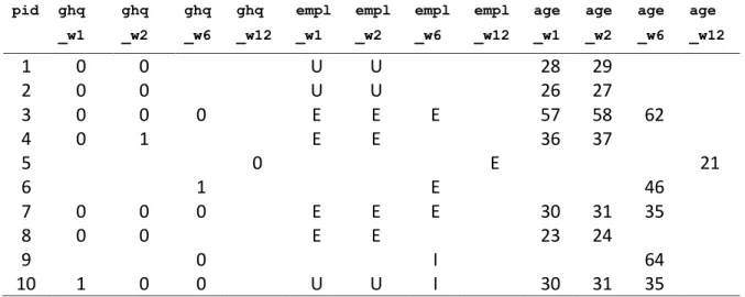
Table 1. Subset of the BHPS data set represented in wide format.

empl and age (predictors) are observed at the different time points as indicated by w1, w2, w6 and w12

pid ghq _w1

ghq _w2

ghq _w6

ghq _w12

empl _w1

empl _w2

empl _w6

empl _w12

age _w1

age _w2

age _w6

age _w12

1

0

0

U

U

28

29

2

0

0

U

U

26

27

3

0

0

0

E

E

E

57

58

62

4

0

1

E

E

36

37

5

0

E

21

6

1

E

46

7

0

0

0

E

E

E

30

31

35

8

0

0

E

E

23

24

9

0

I

64

10

1

0

0

U

U

I

30

31

35

Table 2 displays subjects 1-5 from table 1 but using the alternative long format. Each row now corresponds to the data on a subject at a particular measurement occasion, which reduces the number of columns/variables at the expense of increasing the number of rows in the data set. For instance, ghq_case is now represented using one variable in conjunction with the subject and wave identifiers pid and wave, respectively.

We also define occasion to indicate the measurement occasion for each subject. There are two features of occasion which should be noted:

first, occasion 1 does not correspond to wave 1 for everyone in the sample because some subjects do not appear until after the first wave; and second, the first record on some subjects is not occasion 1 because of missing data on the analysis variables at earlier occasions.

Note that we have defined two employment status variables here: empl is the subject’s employment status at that occasion; and empl1 is employment status at occasion 1. Both age1 and empl1 are subject-level variables whose values are fixed across occasions for the same subject.

Table 2. Subset of the BHPS data set represented in long format

pid wave occasion ghq_case empl age empl1 age1

1 1 1 0 Unemployed 28 Unemployed 28

1 2 2 0 Unemployed 29 Unemployed 28

2 1 1 0 Unemployed 26 Unemployed 26

2 2 2 0 Unemployed 27 Unemployed 26

2 3 3 0 Unemployed 28 Unemployed 26

3 1 1 0 Employed 57 Employed 57

3 2 2 0 Employed 58 Employed 57

3 3 3 0 Employed 59 Employed 57

3 6 6 0 Employed 62 Employed 57

4 1 1 0 Employed 36 Employed 36

4 2 2 1 Employed 37 Employed 36

5 12 5 0 Employed 21 Employed 16

The unbalanced nature of our data can be seen in table 1 and table 2: ghq_case and employment status are not observed for every subject at every occasion. While this is obvious from the wide

3 Why Use Longitudinal Data?

Now that we have seen what a longitudinal data set looks like and discussed some of its features, we recap on the advantages of longitudinal over cross-sectional data.

The first advantage is that longitudinal data allow us to establish the temporal ordering of events. Suppose that we measure mental health and employment status in two waves of a longitudinal panel survey. The mental health of each participant is measured using the GHQ-case variable introduced in Section 2, and the employment status of each participant is classified as either employed (E), unemployed (U) or inactive (I). We can denote employment status at the first and second waves by the categorical variables and , respectively, and GHQ-case at the first and second waves by and , respectively. The longitudinal design allows us to establish with certainty that and are measured before and . The time ordering means that neither nor can have caused or , and longitudinal models with ‘reverse causation’ – in which, say, predicts – can be excluded from consideration.

But this does not mean that longitudinal data automatically gives us the answer to causal questions such as “If I change someone’s first-wave employment status then what will happen to his second-wave mental health ?” To answer such questions definitively, the data need to come from a longitudinal experimental design, or be adjusted appropriately for confounding bias. For a simple example of a longitudinal experimental design, consider an experiment where we measure the mental health of each participant at wave one, , and then randomise each subject to one of the three employment status groups to obtain . If the subjects all keep their randomised employment status during the follow-up period until is measured, then the differences in the proportions of GHQ cases between the three employment status groups are ‘causal estimates’ of employment effect. While an experiment like this would clearly be difficult to implement, the main message is simply this: longitudinal data can help rule out models with reverse causation, but do not guarantee that causal relationships can be estimated.

The second advantage of longitudinal data is that the repeated measurements can be used to improve the precision of our estimates. The

argument we set out here comes from Zeger and Liang (1992), who illustrated their point using a simple experiment much like the one just described. So keep in mind the hypothetical experiment where

is randomised employment status, but suppose that mental health at each wave, and , is measured using the raw GHQ score rather than the GHQ-case indicator. Zeger and Liang showed that the causal effect of employment status can be estimated using the difference score (i.e. the difference ), and calculating the difference between the mean difference scores in each of the three employment categories. Not only is this estimate unbiased, it is more precise (i.e. has smaller standard errors) than simply taking the differences between the means of . The improved precision comes about because measures on the same individual, even at different points in time, are typically positively associated; the general term used to describe positive associations between measurements on the same individual is ‘autocorrelation’. More generally, however, difference scores cannot be used when we have more than two measurements, which is why we need formal longitudinal data methods to allow for autocorrelation and to improve parameter estimation.

The third advantage of longitudinal data is that within-subject changes, or growth, over time can be explicitly modelled along with the outcome’s relationship with time-varying predictors.

4 Population Average and Subject

Specific Models

In this section, we will provide a brief review of both population average (PA) and subject specific (SS) models. To help introduce some of the fundamental differences between PA and SS modelling, we introduce each type of model for the more familiar linear case, before moving onto non-linear logistic models.

4.1 PA linear models

particular wave. In section 6, we discuss the choice of time for our application, but for now we talk simply in terms of time and time-points.

So for subject and time , it might be tempting to use the standard linear model

where is the outcome variable (which would be the raw GHQ score in our illustrative example) and represents the predictor variable(s). It is typically assumed that the residual is normally distributed with variance .

There is one model equation defined for each subject at each time-point. The reason we cannot simply fit this model to the longitudinal data is because it assumes that all the residuals are independent of each other, but we know that all residuals on the same subject are not independent because of autocorrelation.

PA models can be specified and estimated so as to account for autocorrelation. A linear PA model comprises two parts. First is the mean of given the covariates

| )

where | ) denotes the mean outcome among those subjects with predictor variables . Notice that no assumption about the distribution of the residuals has been made.

It turns out that we can estimate the parameters of the PA model provided we specify something about the residual distribution. In fact, it turns out that we only need to specify the (auto)correlation between the residuals The autocorrelation structure is specified simply through the choice of ‘working correlation matrix’ which constitutes the second part of the PA model. We discuss specification of the working correlation matrix in section 4.3.

4.2 PA logistic models

For binary outcomes, one would generally choose a logistic or probit model. We focus on the former because its parameters are conveniently interpreted as log-odds ratios.

As with the PA linear model above, a PA logistic model has two components. The first component can be written as

| )

where ) ⁄ ) is the usual logit ‘link’ function for any probability between 0 and 1. In the context of our example, this means that the log-odds of being a GHQ case is linearly related

to employment status and the other predictor variables.

This is identical to the expression for the standard logistic model apart for the subscript, but we cannot fit the standard logistic model to longitudinal data. There does not appear to be a residual specified in the model above, but there is a hidden residual, and in the standard model these are all assumed to be independent.

The reason we cannot see the residual is because it is hidden from us, but we specified it implicitly when we chose to use the logit link. To show where it is, we note that the logistic model can be represented using latent variables, where there is a continuously distributed outcome variable hidden from us for which we observed only whether its value is positive (i.e. ) or negative ( ). It is further assumed that the hidden outcome variable follows a linear model which depends on the same predictor variable(s) as above and a hidden residual that is logistically distributed. The (standard) logistic distribution in question is a symmetric continuous distribution with a mean of 0 and a variance of 3.29 (the probit model, on the other hand, is based on the assumption that the hidden residuals are normally distributed with mean 0 and variance 1). The 3.29 value emerges again when we discuss the difference between the PA and SS coefficients in section 5.

Hence, we complete the specification of the PA logistic model by specifying the working correlation matrix for the hidden residuals. However, we cannot estimate these residuals as we can for linear models because they are hidden, and we must assume that they all have equal variance (i.e. are homoskedastic).

4.3 Fitting PA models

In short, GEE is a two-stage method in which the autocorrelation structure is treated as a nuisance to be adjusted for. Stage 1 of GEE involves estimating the ‘working correlation matrix’, the structure of which the user must specify prior to estimation; to specify this matrix correctly, the user must declare the occasion variable. Stage 2 of GEE uses the estimated working correlation matrix to adjust the estimates of the logistic model parameters and standard errors for autocorrelation.

For PA linear models, the structure of the residual autocorrelation can be estimated from the data, and used to choose the working correlation matrix. However, as we have discussed, there is no way of doing this for PA logistic models because the residuals are hidden from us (while we can estimate the autocorrelation between the binary outcomes, this is not generally the same as that for the residuals). Instead, we can fit the model using GEE with different working correlation matrices, and use an appropriate goodness-of-fit criterion to establish which is best.

The four main types of working correlation matrix structure are:

 Independence: The residuals are mutually independent (equivalent to a standard logistic regression model). Without adjustment, the standard errors obtained using this method will be too small unless there is no or very little autocorrelation.

 Exchangeable: Every pair of residuals on a subject has the same correlation so that, for example, the residuals at occasions 1 and 2 have the same correlation as the residuals at occasions 3 and 5, and so on; this is also known as ‘compound symmetry’.

 Autoregressive: The correlation decreases exponentially as the time between measurements increases, so that if is the correlation between residuals one occasion apart, then is the correlation between pairs of residuals two occasions apart, and so on, getting smaller and smaller as the gap increases.

 Unstructured: The correlation between a particular pair of residuals is different to that for all other pairs. So the residuals at occasions 1 and 2 have correlation , which is distinct from the correlation between residuals at occasions 2 and 3

, and so on.

We herein refer to a PA model fitted using GEE with an exchangeable working correlation matrix as

the ‘exchangeable’ PA model, with the

‘independent’ PA, ‘autoregressive’ PA, and ‘unstructured’ PA models similarly defined.

The exchangeable and autoregressive working correlation matrices both involve one parameter, , whereas the unstructured matrix (as its name suggests) makes no assumptions about structure but involves ) parameters to represent the autocorrelation between the residuals at T occasions. For instance, in our example, there are up to 18 measurement occasions and so the unstructured working correlation matrix has ⁄ parameters. In practice, the unstructured working correlation matrix should always be used for examples involving few measurement occasions, but when there are many occasions it is often inestimable (i.e. the fitting routine is unable to estimate it and will output only an error), although this is not the case in our illustrative example.

One way to choose between different matrices is to use the quasi-likelihood information criterion (qIC) (Pan 2001). The qIC comprises an overall measure of goodness-of-fit and a penalisation for model complexity (i.e. the number of parameters in the working correlation matrix and predictor variables in the model). Hence, for two models with the same goodness-of-fit, the qIC will indicate that the model with the fewest parameters is to be preferred. We discuss how to use qIC further on in Section 6.

4.4 SS linear models

Subject specific (SS) models handle

autocorrelation by including a unique ‘effect’ for each individual subject, which is separate from the occasion-specific residual. In contrast to PA models, there are many different ways of specifying the individual-level effects in SS models, and many different ways of estimating the resulting models.

An example of a SS linear model is a two-level random intercepts model with the individual subject at level two and the occasion at level one. It can be written as

independent of each other (and of ) just as for standard regression models.

The residuals can be thought of as representing the combined effect on mental health of the variables omitted from the model. Hence, a random effect accounts for autocorrelation by ex-plaining the omitted time-invariant variables for an individual subject. This is the key difference between SS and PA models: the PA model makes no explicit assumptions about any random effects or between-subject differences. However, the random intercepts model implies the same exchangeable autocorrelation structure as the exchangeable PA model.

Random intercept models can be extended through the addition of ‘random slopes’. To construct a random slopes version of the model above, we would specify (the random intercept) and the random slope , where is the same random effect as before, and is another normally distributed random effect, which can be correlated with . This model allows the effect of on mental health to vary between subjects. In practice for longitudinal data, it is common to have a covariate corresponding to the time-point to model ‘growth’ in the outcome over the study; a random slope for time thus allows each subject to follow a different growth trajectory or trend.

In our example in Section 6, where we use age to index time, we consider a simple linear growth relationship between age and mental health, where the log-odds of poor mental health can increase or decrease linearly with age, at the same rate (random intercept) or different rates (random slope) for each individual. More complex relationships between the outcome and time can be modelled, for example, by including quadratic or higher order polynomial terms (e.g. by including age2

, age3

, etc. in our example). Each additional parameter can be made subject specific by allowing it to vary randomly across individuals in a random slopes model. However, each added parameter (fixed or random) complicates the model and may make its conclusions more difficult to interpret. As a rule, we therefore recommend that readers consult manuals and worked examples of such models before developing complex random slopes models.

Random slopes models allow more complex

autocorrelation structures than the simple

exchangeable autocorrelation allowed by random intercepts models. The correlation between pairs of residuals is allowed to depend on the time (as we have chosen to index it in the model) between measurement occasions in a complex fashion, but there is no direct correspondence between the autocorrelation structure implied by a random slopes model and the autoregressive or un-structured autocorrelation structures we can specify directly for PA models.

4.5 SS logistic models

The logistic random intercepts model is likewise written

| )

where again is the random intercept, and the occasion-level residual is implicit in the choice of the logit link. The individual-level residual is normally distributed as before and plays the same role as for linear models, namely, accounting for autocorrelation due to the omitted characteristics of the individual subject common to all time points.

The two variance components (for occasion and individual) are on two different scales and cannot be compared directly. However, a useful measure is the intra-class correlation (ICC), which is the proportion of the total residual variation that is due to differences between individuals. The ICC is output by most routines for fitting random intercepts models, but it cannot be estimated from PA models.

The use of a non-linear ‘link’ function between the probability and the linear predictor on the right hand side leads to a difference in interpretation between the parameters of the SS models and PA models. We discuss this distinction in more detail in Section 5, and again in the context of our data example in Section 6.

4.6 Fitting SS models

likelihood estimation method available with the xtmelogit procedure in Stata, that is, a Gauss-Hermite adaptive quadrature approximation with 7 integration points.

5 Why is there a difference between

SS and PA coefficients?

We noted in Section 4 that the coefficients in SS and PA logistic models have different interpretations. Furthermore, as we will see in the analysis presented in Section 6, the SS coefficients will generally be larger than the PA ones. In this section, we use a simulated data set to explain why this is the case for random intercepts SS and PA exchangeable models, which are consistent in this context.

To begin, just consider one time point t in a longitudinal study. For each subject i we have a binary variable and a continuous predictor at that time point. The predictor variable is uniformly distributed and so is equally likely to take any value between 0 and 10. Now suppose that the relationship between the predictor and the binary outcome at a given time follows the SS random intercepts model

| ) where the random effect is normally distributed with mean 0 and variance 2. This model tells us how the log-odds of a positive response for any subject varies with , which we will denote as .

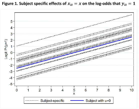
Figure 1

.

Subject specific effects of

on the log-odds that

From figure 1, we can see how the SS log-odds increase with for 20 randomly selected subjects. The relationship is linear, and the blue line shows the log-odds for the mean subject ), which happens to equal the log-odds for the median subject because is normally distributed. As this is a random intercepts model, the other lines are parallel to that for the mean/median subject (the slopes can also vary for different subjects under a random slopes model).

However, the situation changes when we consider the relationship between the probability of a positive response and because the relationship

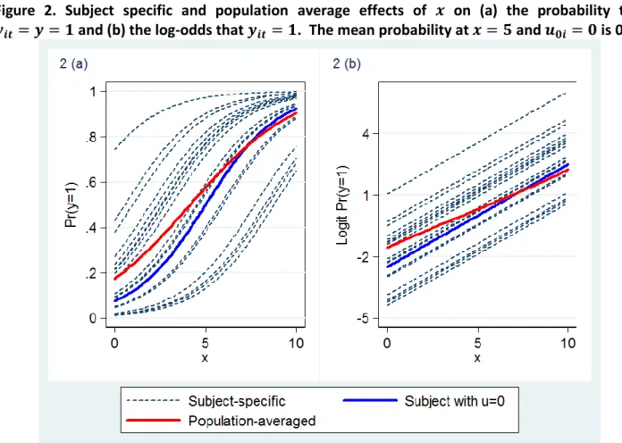
Figure 2. Subject specific and population average effects of

on (a) the probability that

and (b) the log-odds that

. The mean probability at

and

is 0.5

Further displayed in figure 2a is the red PA curve, which is obtained by taking the mean of the SS probabilities at each value of . The SS curve for an individual at the mean of the random effects distribution ) is also shown in blue. Why are the two curves different? It is because of the non-linearity of the logistic function that the probability for the mean subject will not equal the mean probability. Instead, the probability at now corresponds to the median probability because, unlike the mean, the median is unaffected by the logistic transformation.

From figure 2a, it can be seen that for values of between 0 and 7, the PA or mean curve lies above the median curve. This is because the greater part of the spread of the SS curves at these values lies above the blue line, which indicates a positive skew and the median probability exceeding the mean probability. For values of greater than 7, however, the greater part of the response-probability spread lies below the median, which pushes the mean below the median.

Figure 2b displays the effects of on the log-odds scale (this plot is identical to figure 1 apart

from the addition of the PA line which was obtained by applying the logistic transformation to the PA probabilities in figure 2a). We can see that the coefficient of from the PA model ) is the slope of the PA line in figure 2b, while the coefficient from the SS model ) is the slope of the SS line for an individual with , and we can see that for most of the time.

The relationship between the PA and SS effects observed in figure 2b holds more generally. It can be shown that the random intercepts SS coefficients are related to the PA coefficients by

_√

coefficients are equal if there is no between-subject variation. The greater the between-subject var-iation, the greater the SS coefficient is compared to the PA one. This relationship can be extended to more complex random effect structures such as random slopes (Zeger, Liang & Albert, 1988).

A consequence of this is that one should not report the SS effect simply because it is larger than the PA effect. It does not mean that the SS model shows a ‘stronger’ effect than the PA model; it simply means that there is between-subject variation: the two measures are equivalent but different. However, we should note that the relationship above is only an approximation, and it is possible for to be close to, or even less than, _{even when the random effect variance is large.}

Finally, although the SS and PA coefficients can be very different, the ratio of a parameter estimate to its standard error will in general be similar for the two models; thus, significance tests will be unaffected by the choice of model.

6 Data Analysis

6.1 Preliminaries

We use the BHPS data introduced in Section 2 to analyse the relationship between mental health and employment status. A suitable longitudinal analysis of these data is important because the relationship is a dynamic one that varies from wave to wave, and a simpler analysis would risk losing important information about variation or change in mental health over time. We conduct a simple analysis here to illustrate the most important points regarding the comparison of PA and SS logistic models, but refer the reader elsewhere for further analyses of the same data (Steele et al., 2013).

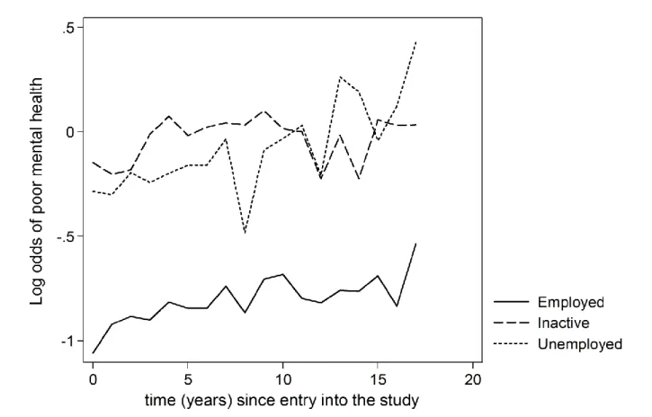
Before carrying out any modelling, we first look at the raw data. In the figures below, we use occasion as a subject specific measure of time for each subject (occasion being annually spaced), and in figure 3 we can see how ghq_case varies over time for each category of empl1. We plot the log-odds of poor mental health (i.e. ghq_case = 1) because it is this that is being modelled by both the PA and SS logistic regression models.

It can be seen from figure 3 that, when looking only at the log-odds of ghq_case at the final occasion, and comparing it with the log-odds at the first, that there is an increase in both the employed and inactive groups, but there is less pronounced change among the unemployed. We can also see that the log-odds of ghq_case varies for all

categories throughout the study period, and this variation cannot be captured without using all the available outcome measures. It is worth emphasising at this point that figure 3 represents the population average log-odds of ghq_case in each employment category, which can be very different to its subject specific equivalent.

Figure 4. Relationship between the log-odds of GHQ ‘caseness’ and the time since entry into the

study by time-varying employment status

Figure 4 shows the relationship between the log-odds of being a GHQ case/having poor mental health and the time-varying employment variable (empl). Comparing figures 3 and 4 highlights that the log-odds of poor mental health among the unemployed increased during the survey. As we shall see later, the difference between the two figures can partly be explained by the change in the employment distribution over the observation period, which confirms the importance of treating employment status as a time-varying predictor. However, we first analyse these data using empl1 as our explanatory variable, and present estimates of the effect of employment status on mental health using PA and SS models.

6.2 Simple models with no time-varying

predictors

To begin, we fit a simple model in which the mental health outcome varies over time but the employment status predictor is that from occasion 1. Using a symbolic ‘pseudo code’ notation, this model can be written as

Log-odds (ghq_case = 1) = intercept + unemployed_1 + inactive_1 + agec_1

represents the constant term (its coefficient is the

intercept ); unemployed_1 and inactive_1

are dummy variables for whether subjects were, respectively, unemployed and inactive on first entry to BHPS; and agec_1 represents the subject’s mean-centred age (that is, the difference between the subject’s age and the sample mean of age) at the first occasion. Hence, in contrast to the left hand side, none of the variables in the linear predictor change over time.

We adjust for age at occasion 1 but note that, in substantive (rather than illustrative) applications, we may wish to adjust for a wider range of variables (for example, to adjust for confounding bias). We use mean-centred age so that can be interpreted as the log-odds of GHQ caseness for an employed subject of mean age. Centring is important for any

continuous predictor variable for which we wish to add a random slope (see section 6.3 for an example).

We now fit the symbolic model introduced above using both the PA and SS approaches. These analyses were conducted using Stata and the following functions: logit for the simple logistic; xtlogit with options pa and robust to fit PA models using GEE; and xtmelogit to fit random effects models using the mle fitting option. The code we used for this data analysis is provided in the supplementary material and the results are presented in table 3.

The robust option uses a ‘sandwich estimator’ that takes into account that the working correlation matrix may be incorrect. All GEE routines will have a robust option (or its equivalent) and this should always be used.

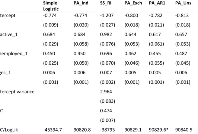
Table 3. Results from fitting the basic model without temporal trend.

Simple Logistic

PA_Ind SS_RI PA_Exch PA_AR1 PA_Uns

Intercept -0.774

(0.009)

-0.774

(0.020)

-1.207

(0.027)

-0.800

(0.018)

-0.782

(0.021)

-0.813

(0.018)

inactive_1 0.684

(0.029)

0.684

(0.058)

0.982

(0.076)

0.644

(0.053)

0.617

(0.061)

0.657

(0.053)

unemployed_1 0.450

(0.025)

0.450

(0.050)

0.696

(0.070)

0.462

(0.046)

0.455

(0.055)

0.487

(0.045)

agec_1 0.006

(0.001)

0.006

(0.001)

0.007

(0.002)

0.005

(0.001)

0.005

(0.001)

0.006

(0.001)

Intercept variance 2.964

(0.083)

ICC 0.474

(0.007)

qIC/LogLik -45394.7 90820.8 -38793 90829.1 90829.6* 90840.5

The first column in table 3 contains the results obtained from fitting a simple logistic model that does not account for autocorrelation. The second column (PA_Ind) contains the results from fitting the independence PA model using GEE, namely, the independence PA. If we do not use the robust option for the GEE, we would expect both sets of estimates to be exactly the same. However, as we have discussed, GEE should always be estimated using robust, and so we can see that the estimated standard errors are larger for the PA independence model, because the autocorrelation in the data has been allowed for.

Next we consider the random intercepts (RI) model (SS_RI) and the exchangeable PA model (PA_Exch). As noted previously, both of these models require that the autocorrelation structure is exchangeable, and both have larger standard errors than the simple logistic model because autocorrelation is accounted for.

Perhaps the most salient feature of table 3 is that the RI model estimates all have larger absolute values than the exchangeable PA model estimates. The estimated PA exchangeable logistic model for person at occasion is

| )

and we can interpret the estimates of the two employment status dummies in the usual manner for logistic models. The odds of being a GHQ case for employed people of mean age at occasion 1 are ) ; the odds ratio of being a GHQ case for the unemployed compared to the employed, conditional on age at occasion 1, is ) , which means that the unemployed are 60 percent more likely to be GHQ cases than the employed; the odds ratio for the inactive relative to the employed is similarly obtained.

If we now look at the estimated random intercepts SS model

| )

where is normally distributed with mean 0 and variance 2.9. The presence of the random effect (the term) means that each individual subject has his own regression equation. Using this model, for subjects with the same value of , the SS odds of being a GHQ case are ) among subjects

employed at the start of the study, and the SS odds ratio of being a GHQ case for unemployed subjects compared to employed ones is ) .

As was discussed in section 5, the odds ratios obtained using RI models are usually larger than those from the exchangeable PA model (Neuhaus, Kalbfleisch & Hauck, 1991), but this is because both are different measures of the same association. It is important to remember that SS model results should not be reported here just because the odds ratio is larger: it does not mean that the SS model has estimated a ‘stronger’ effect, it just means that the two coefficients are different measures of association (even though both odds ratios equal 1 if there is no association).

The two approaches are complementary and the most relevant depends on the focus of a particular analysis. In our example, the effect of employment status can legitimately be reported as either a population average or a subject specific effect. If employment status were randomised and fixed throughout the study, as in our hypothetical example in Section 3, then the PA estimate would be akin to a ‘causal odds ratio’, summarising the effect of employment status across the experimental population rather than for any particular subject. On the other hand, the SS estimate pertains to the effect of employment status on any given subject, that is, what will happen to that subject if he changed only his employment status. (Of course, it is important to remember that estimates based on non-experimental data will only be causal if confounding bias has been adjusted for.)

Table 4. Population average estimates from the exchangeable PA model as per table 3 and

derived from the random intercepts logistic model

RI

PA_Exch

Employed_1

-0.848

-0.800

Inactive_1

0.690

0.644

Unemployed_1

0.489

0.462

Unfortunately, there is no rule for converting PA parameters to SS ones because a PA model can correspond to many different SS models. In some quarters, this is perceived to be a strength of the PA approach, because no assumptions appear to have been made about the distribution of the residuals and random effects. However, a counter-argument to this is that these assumptions are hidden from us and cannot be inspected, whereas the assumptions of SS models are clear and can be relaxed if more advanced SS modelling approaches are used.

While the random intercepts and exchangeable PA models allow for the same type of autocorrelation structure, it is always advisable to explore alternative autocorrelation structure assumptions to improve the estimation accuracy further and ensure the estimates lie as close as possible to the truth. The robust option inflates the standard errors, but the estimates may be far too large if the choice of working correlation matrix is poor. For PA models, this can be done by fitting PA models using GEE with two, more complex, autocorrelation structures: the autoregressive and unstructured PA models. These results are displayed in the final two columns of table 3.

We can see from table 3 that the absolute values of the unstructured PA (PA_Uns) model estimates are larger than those for the autoregressive PA (PA_AR1) model, with the exchangeable PA model estimates lying somewhere between the two. We can use the qIC to choose between the three PA, where the smallest qIC indicates the ‘best’ fitting model in terms of the balance between goodness-of-fit and simplicity. The code used to calculate the qIC is given in the supplementary material.

The first point to note is that the qIC of the autoregressive PA model is not directly comparable to that for the other two. This reflects that GEE estimation using the autoregressive correlation

structure, as implemented in Stata, requires that all the individuals in the data set are observed for consecutive occasions and as such does not handle gaps between occasions (users of other software must check if the situation is the same for them). From the data summary in table 3, we can see that only 57,592 (out of 72,173) observations on 7,479 (out of 9,192) individuals have been used. To be comparable, all three PA models should be fitted to the same sample so that the qICs can be compared. We take this approach in the analyses to follow (all of the models are fitted to the reduced sample of 7,479 observations), but simply exclude the autoregressive PA model for consideration here.

6.3 Models that allow for time-varying age

How can we relax the exchangeable

autocorrelation structure implied by the random intercepts SS model? The approach we follow is to extend the linear predictor of the simple model to explain changes in mental health over time. The rationale for this is that the exchangeable (or even independence) autocorrelation structure becomes more plausible as we explain more systematic variation through the linear predictor.

To do this, we can extend the model to allow a subject’s log-odds of GHQ caseness to vary as they age, and therefore capture some of the trend in log-odds we saw in figure 3. By doing this, we assume that changes in mental health over time are driven primarily by a subject’s age; the impact of when subjects were born (‘cohort effects’) and the

calendar year when mental health was measured (‘period effects’) is thus taken to be less important. Using the symbolic notation, this model is written as

Log-odds (ghq_case = 1) = intercept + unemployed_1 + inactive_1 + agec

recalling that we use mean-centred age agec, which increases with time and replaces the first-occasion age variable used in section 6.2.

The results obtained from fitting this model using different PA and SS approaches are presented in table 5. Recall that, in contrast to the results in the previous table, we fit the different PA and SS models to the 7,479 individuals in order to make the other results comparable to those obtained using the autoregressive PA model.

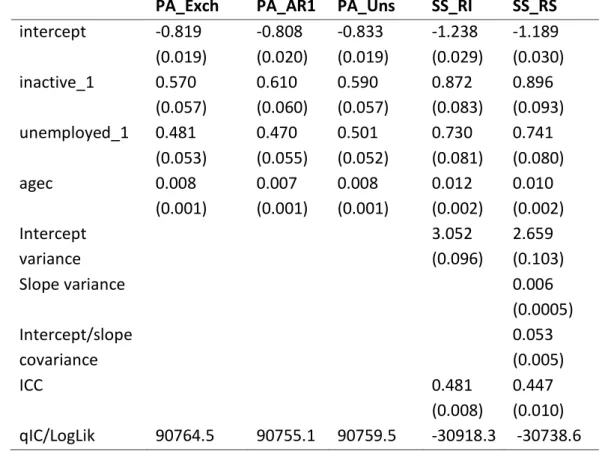
Table 5. Results from fitting the model with an age trend.

PA_Exch

PA_AR1 PA_Uns

SS_RI

SS_RS

intercept

-0.819

(0.019)

-0.808

(0.020)

-0.833

(0.019)

-1.238

(0.029)

-1.189

(0.030)

inactive_1

0.570

(0.057)

0.610

(0.060)

0.590

(0.057)

0.872

(0.083)

0.896

(0.093)

unemployed_1

0.481

(0.053)

0.470

(0.055)

0.501

(0.052)

0.730

(0.081)

0.741

(0.080)

agec

0.008

(0.001)

0.007

(0.001)

0.008

(0.001)

0.012

(0.002)

0.010

(0.002)

Intercept

variance

3.052

(0.096)

2.659

(0.103)

Slope variance

0.006

(0.0005)

Intercept/slope

covariance

0.053

(0.005)

ICC

0.481

(0.008)

Focussing on the SS_RI model (penultimate column in table 5), we note that the parameter for agec in the SS model describes a within-subject trend in mental health with age. More generally, SS models are the more natural choice if within-subject characteristics of growth are the focus of the analysis. The corresponding effect in the PA models is a measure of change in the population average and less useful for describing subjects’ growth.

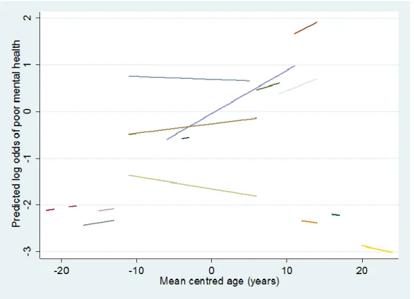
We can extend the random intercepts model by allowing a random slope for the effect of agec. It is sensible to consider this model because, as we can see from figure 5, there is substantial between-subject variation in the time trend. The variance of the random slope measures between-subject variation in age trend, and allows for a more complex autocorrelation structure than the random intercepts model. The use of mean-centred age is particularly important here because the random intercept variance can be interpreted as the between-individual variance at the mean age (rather than age zero), and the intercept-slope covariance is between an individual subject’s log-odds of GHQ caseness at the mean age and his rate

of change. Centring continuous predictor variables with random slopes can also stabilise the fitting of these models.

The results from fitting the random slope model are displayed in the final column of table 5 (SS_RS). The likelihood ratio test of including the random slope is obtained by taking the difference between the log-likelihoods for the random slopes and intercepts models and multiplying it by to get , which, compared to a chi-square on 2 degrees of freedom, reveals substantial evidence to support its inclusion. The random slopes model allows a different effect of agec for each individual, which implies that two different individuals will experience different rates of change in the odds of suffering from poor mental health with age (even if they are in the same employment category). If we were to convert the SS parameter to a PA one using the same method as used for table 4, we would find that the relationship would be quadratic rather than linear (due to the presence of both random intercept and random slope variance, as well as the covariance between the two random terms), which further emphasises that PA models say little about within-subject change.

6.4 Models that allow for time-varying

employment status

Finally, we complete the picture by including employment status as a time-varying variable to utilise fully the information contained in the data. Many of the sample subjects changed employment status at least once during the study with the proportion of men in each employment category varying between waves.

To model time-varying employment status, we include empl as a predictor rather than empl1. We assume that this prevents reverse causation because empl is asked retrospectively, and the subject’s current employment status will have been determined at a point prior to the current occasion. Conversely, the subject’s mental health varies from day to day, and is measured on the day of the study.

Using our symbolic notation, we can write this model as

Log-odds (ghq_case = 1) = intercept + unemployed + inactive + agec

The variable agec is included on the basis of our previous investigations. While ghq_case is measured at the time of the survey, employment status is actually determined in the between-time point interval, and so – for the purposes of this application – we take it to be temporally antecedent to the mental health measure. However, we discuss in Section 7 the use of ‘lag’ variables (namely, including employment status from time points prior to the current one) as a further guard against reverse causation.

As previously, we fitted five different models to the same dataset: exchangeable PA (PA_Exch), autoregressive PA (PA_AR1), unstructured PA (PA_Unst), random intercepts (SS_RI), and random slopes (SS_RS).

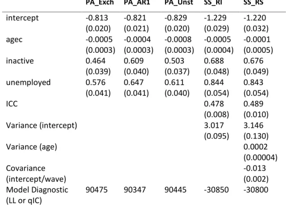
Table 6. Results from fitting the model with temporal trend and time-varying employment.

PA_Exch PA_AR1 PA_Unst SS_RI SS_RS

intercept

-0.813

(0.020)

-0.821

(0.021)

-0.829

(0.020)

-1.229

(0.029)

-1.220

(0.032)

agec

-0.0005

(0.0003)

-0.0004

(0.0003)

-0.0008

(0.0003)

-0.0005

(0.0004)

-0.0001

(0.0005)

inactive

0.464

(0.039)

0.609

(0.040)

0.503

(0.037)

0.688

(0.048)

0.676

(0.049)

unemployed

0.576

(0.041)

0.647

(0.041)

0.611

(0.040)

0.844

(0.054)

0.843

(0.054)

ICC

0.478

(0.008)

0.489

(0.010)

Variance (intercept)

3.017

(0.095)

3.146

(0.130)

Variance (age)

0.0002

(0.00004)

Covariance

(intercept/wave)

-0.013

(0.002)

Model Diagnostic

(LL or qIC)

All the estimates from the various PA models are similar to each other apart for the inactive category of employment, the coefficient of which seems to be influenced by the working correlation structure (although the qIC indicates that the autoregressive PA seems to be the best model). For the SS models, the random slopes model is a better fit to the data than the random intercepts model, providing support towards growth-type models with individual-specific effects.

7 Discussion

In this tutorial, we have considered the differences between using population average (PA) and subject specific (SS) models for the analysis of longitudinal data.

In short, PA models are more appropriate for estimating the average effects of predictors (in our case, employment status) on outcomes. The parameters of PA models are most relevant to measuring the effect of time-invariant predictors; an example of this is in experimental settings (or observational settings where it can be justified that confounding bias has been adjusted for) for estimating the ‘average’ effects of predictor variables which correspond to a ‘treatment’ or ‘exposure’ of interest. However, PA models make no (explicit) assumptions about the distribution of the random effect, and so cannot be used to estimate between-subject variation or between-subject-level residuals. The nature of GEE estimation for PA models means we cannot use proper goodness-of-fit statistics based on likelihoods, and so must rely on ad-hoc tools like qIC.

The SS models we consider allow a different model for each subject through the use of random effects. In experimental/confounding-adjusted set-tings, the parameters of these models correspond to the effect of the treatment/exposure on each subject. If the target of the analysis is growth, or more general within-subject change, then SS models are more appropriate than PA models (because, in a nutshell, changes in averages are not the same as average changes for non-linear models). Random slopes can be used to increase the complexity of the SS models (although these models can be difficult to fit) at the expense of modelling assumptions like normality of the random effects. An advantage of SS models is that PA effects can be estimated using marginalisation. For logistic models with normal random effects, one can always use the formulae discussed in sections 5 and 6. Conversely, it is impossible to obtain estimates of the

SS parameters from a PA model because there are many SS models that correspond to the same PA model (Lee and Nelder, 2004).

In our application, we handled the missing data

problem by excluding any subject-occasion

contributions with missing values from the data set. GEEs require that the data are Missing Completely At Random (MCAR) such that the missing values arose in a manner completely independent of the variables in the analysis2. On the other hand, SS models require only that the data are Missing at Random (MAR) such that the missing values arose in a manner that depends only on the variables we happen to observe. More generally, weighted GEE estimation can be performed to allow MAR data, and multiple imputation methods can be used for either approach to ‘fill in’ incomplete data sets under the MAR assumption (Carpenter & Kenward, 2013).

One of the powerful features of longitudinal data is that models with reverse causation can be avoided. In our application, we argued that using employment status to predict mental health, where both were measured at the same occasion, precluded reverse causation, but this argument may be unconvincing to some. To protect against this, one may use ‘lagged’ employment status from the previous occasion as a predictor instead; another example, used by Steele et al. (2013), is to use the between-occasion change in employment status as the predictor.

Acknowledgements

We thank George Leckie for providing Stata code to generate the figures presented in section 5.

Supplementary Material

Stata .do file corresponding to the analyses is available online as a Supplementary File.

The data used in the analyses are available on request from the authors. However, as we use BHPS data, anyone making such a request must also provide evidence that they are registered with the ESRC Data Archive.

References

Baltagi, B.H. (2008). Econometric Analysis of Panel Data (4th edn.). Chichester: Wiley.

Bollen, K.A., & Curran, P.J. (2005). Latent Curve Models: A Structural Equation Perspective. New Jersey: Wiley.

Carpenter, J., & Kenward, M. (2013). Multiple Imputation and its Application. London: Wiley. Cui, J. (2007). QIC Program and Model Selection in GEE Analyses. The Stata Journal 7, 209-220.

Goldberg, D.P., Gater, R., Sartorius, N., Ustun, T.B., Piccinelli, M., Gureje, O., & Rutter, C. (1997). The validity of two versions of the GHQ in the WHO study of mental illness in general health care. Psychological Medicine, 27, 191-197

ISER. (2010). British Household Panel Survey: Waves 1-18, 1991-2009 (7th edn.). University of Essex, Institute for Social and Economic Research [original data producer(s)], Colchester, Essex: UK Data Archive [distributor].

Lee, Y., & Nelder, J.A. (2004). Conditional and Marginal Models: Another View. Statistical Science 19, 219-238. Liang, K-Y., & Zeger, S.L. (1986). Longitudinal Data Analysis using Generalized Linear Models. Biometrika 73,

13-22.

Neuhaus, J.M., Kalbfleisch, J.D., & Hauck, W.W. (1991). A Comparison of Cluster-Specific and Population-Averaged Approaches for Analysing Correlated Binary Data. International Statistical Review 59, 25-35.

Pan, W. (2001). Akaike’s Information Criterion in Generalized Estimating Equations. Biometrics 57, 120-125. Robins, J.M., Greenland, S., & Hu, F-C. (1999). Estimation of the causal effect of a time-varying exposure

on the marginal mean of a repeated binary outcome. Journal of the American Statistical Association 94, 687-700.

StataCorp. (2011). Stata Statistical Software: Release 12. College Station, TX: StataCorp LP.

Steele, F., French, R., & Bartley, M. (2013). Adjusting for selection bias in longitudinal analyses using simultaneous equations modelling: The relationship between employment transitions and mental health. Epidemiology (in press).

Zeger, S.L., & Liang, K-Y. (1986). Longitudinal Data Analysis for Discrete and Continuous Outcomes. Biometrics 42, 121-130.

Zeger, S.L., Liang, K-Y., & Albert, P.S. (1988). Models for Longitudinal Data: A Generalized Estimating Equation Approach. Biometrics 44, 1049-1060.

Zeger, S.L. & Liang, K-Y. (1992). An overview of methods for the analysis of longitudinal data. Statistics in Medicine 11, 1825-1839.

Endnotes

1 _{For a logistic model, the SS parameters can be marginalised by using the Zeger, Liang & Albert (1988) approximation:}

_√

where represents the vector of SS parameter estimates, the corresponding vector of PA parameter estimates

for observation i, and represents the variance of the random part of the linear predictor for observation i,which can be different for each individual when random slopes are fitted.

2 _{GEE can be used for Missing At Random (MAR) data but the working correlation matrix cannot be consistently}