UNSUPERVISED DATA AND HISTOGRAM CLUSTERING USING
INCLINED PLANES SYSTEM OPTIMIZATION ALGORITHM
MOHAMMAD HAMED MOZAFFARI
AND SEYED HAMID ZAHIRI1
Department of Electrical Engineering, Faculty of Engineering, University of Birjand, Birjand, Iran e-mail: [email protected]
(Received September 25, 2013; revised January 22, 2014; accepted March 11, 2014)
ABSTRACT
Within the last decades, clustering has gained significant recognition as one of the data mining methods, especially in the relatively new field of medical engineering for diagnosing cancer. Clustering is used as a database to automatically group items with similar characteristics. Researchers aim to introduce a novel and powerful algorithm known as Inclined Planes system Optimization (IPO), with capacity to overcome clustering problems. The proposed method identifies each agent used in the algorithm to indicate the centroids of the clusters and automatically select the number of centroids in each time interval (unsupervised clustering). The evaluation method for clustering is based on the Davies Bouldin index (DBi) to show cluster validity. Researchers compare known algorithm on series of data bases from various studies to demonstrate the power and capability of the proposed method. These datasets are popular for pattern recognition with diversity in space dimension. Method performance was tested on standard images as a dataset. Study results show significant method advantage over other algorithms.
Keywords: Davies Bouldin index, histogram; image processing, inclined planes system optimization, soft computing, unsupervised clustering
INTRODUCTION
Within the last decade, natural computing has been recognized as a novel approach to solve real life prob-lems inspired by nature. In this field, scientists have proposed several algorithms such as Particle Swarm Optimization (PSO) by Kennedy and Eberhart (1995); Genetic Algorithm (GA) by Tang et al. (1996) and other algorithms to overcome problems of optimization, classification, data analysis and clustering (Lezoray, 2003; Jackson et al., 2009).
Clustering is a way of finding the hidden data struc-ture and refers to a set of data with shared common properties as separate entities. A suitable clustering method helps classify a large group of N-data items with P-dimensional features, to be placed into smaller groups, where each group will share similar properties with its items, and dissimilarity with items in the other groups. Clustering algorithms are used in various fields of science to solve engineering problems specific to bioinformatics (Krikpatrick et al., 1983; Jain et al., 1999; Xu and Wunsch, 2005; Dembele, 2008).
Numerous clustering methods have been designed including: Hierarchical clustering, Fuzzy clustering, Nearest Neighbor (KNN) by Altman (1992) and K-means by Sang (2012). Traditional clustering methods
perform their duty perfectly up to a certain point and until some difficulties arise with unknown number of clusters in a database showing numerous dimensions. This rapid growth of scientific information will inevi-tably pose problems with an expanded volume of scientific data (Zahiri, 2010).
New clustering methods are mainly aimed at the compilation of past methods and heuristic algorithms. Various forms of heuristic algorithms were initially introduced decades ago. The most popular and famous algorithm was Simulated Annealing (SA) by Krik-patrick et al. (1983), Artificial Immune System (AIS) by Farmer et al. (1986), Ant Colony Optimization (ACO) by Dorigo (1992), the Genetic Algorithm (GA) by Tang et al. (1996), and there were Particle Swarm Optimization (PSO) by Kennedy and Eberhart (1995) and Harmony Search (HS) by Geem et al. (2001).
deve-loped by simulating the social behavior in flock of birds at migration. Harmony Search (HS) algorithm mimics musician’s behaviors in the process of impro-visation. Stochastic behavior and using randomized phenomena are a usual strategy for these algorithms to simulate natural characteristics similar to their actual pattern, while in some other algorithms like Central Force Optimization (CFO), there is no randomization. CFO is a deterministic and heuristic algorithm based on the metaphor of gravitational kinematics (Formato, 2007; Mozaffari et al., 2013).
Population-based methods are inspired by the social interactions dynamics between individuals. For instance, PSO simulates group cooperation in flocks of birds where each particle tries to move toward the best position by using its own previous experience guided by the neighboring particles. Sharing infor-mation in population-based algorithms is a common strategy when each individual shares its information with others in order to guide the swarm to its goal of “optimum position”. This cooperation between particles is known as swarm intelligence, with a significant improving effect on the algorithms’ results (Kennedy and Eberhart, 1995; Mozaffari et al., 2013).
In this paper, Inclined Planes system Optimization (IPO) algorithm is used to cluster a number of stan-dard datasets. The IPO clustering process is evaluated in each time interval to determine the correct number of clusters with a validity criterion function. Various validity functions are designed by researchers such as Hubert and Levin, Likelihood, SSI, Marriot and others (Dimitriadou et al., 2002; Chou et al., 2004; Omran et al., 2005).
Researchers used Davies-Bouldin index (DBi) as an objective and criterion for IPO algorithm clustering process (Davies and Bouldin, 1979). In another study, each of the IPO algorithm agents called “tiny ball” represented the number and position of cluster cen-troids in the problem space. Algorithm was initialized step by step, where each ball length was randomly changed to find the best one by using minimum DB index and a threshold for each time interval. This process was repeated until terminated criterion was reached and the best DB index value occurred (Omran and Salman, 2005).
In this study, performance of the proposed method is based on 4 standard datasets and 3 histograms from standard reference images to reveal its effectiveness on reliability and power of the method on clustering problems in similar applications.
INCLINED PLANES SYSTEM
OPTIMIZATION (IPO)
The IPO algorithm design was built on the sliding motion dynamic along a frictionless inclined surface. Agents or “tiny balls” in this algorithm, similar to the particles in PSO or ants in ACO have the capacity to search the problem space and find the nearest optimal solution. These tiny balls reach a certain height for fitness.
The IPO algorithm is designed to find the opti-mum answer for engineering problems and inspired by the phenomena of “losing potential energy”. For instance, each ball has three specifications of position, height and angle in relation to other balls. The po-sitions these balls assume create feasible solutions for the problem using the objective function to calculate the height for each ball.
To estimate an inclined plane, IPO method uses straight lines to cross from the centroid of one ball to the centroids of other balls. To minimize the problem, formed angles between the straight lines and the horizontal line are calculated to find the direction and acceleration of each ball. The position of i-th ball from np balls system can be defined as shown in Eq. 1
with a restriction. Here Xi is the decision variable, k is
the coordinate number and nd is the space dimensions.
The position of i-thball in k-th dimension is presented by xi
k .
d k i p n i k i i i n k x x x n i for x x x X d 1 , , , 2 , 1 , , , , , max min1
(1)
The proposed method of IPO tends to find mini-mum location of objective function f(X) defined by the problem space. For each ball, IPO parameters are calculated in separate dimensions. The angle between the i-th ball and j-th ball at the time interval of t is calculated in the following equation, where fi(t) and
fj(t) are the objective function values (heights) for the
i-th and j-th ball in time t respectively.
j i n j i and n k for t x t x t f t f t p d k j k i i j k ij , , , 2 , 1 , , , 1 , tan1 .
(2)without consideration for the movement of other balls. It means acceleration is calculated between two se-quential time intervals and later, the acceleration amount and direction are calculated as shown in Eq. 3 and Eq. 4 below, where U(.)is the unit step function.
,
(3)
j i n j i and n k for t t f t f U t a p d k ij n j i j k i p
, , , 2 , 1 , , , 1 sin . 1 .
(4)
0 0 0 1 w w w UHere ɸijk is the angle between the i-th ball and j
-th ball at t (time interval). For updating each ball's position at every time interval, the law of motion with constant acceleration is used where rand1 and rand2
are two random weights with uniform distribution at interval [0, 1] to give a stochastic characteristic to IPO algorithm. It is important to notice that in heuristic algorithm adopting a natural phenomenon is followed by certain modifications on the relations. For example, gravitational constant in GSA (G0) is changed by
adaptation at each time iterations. Thus, the term 1/2
seems negligible in the law of motion with constant acceleration.
As shown below, vi k
(t) is the velocity of ball i in dimension k, at time t. The k1 and k2 are two changing
constants with time as seen in Eq. 7 and Eq. 8. The vi k
is defined as Eq. 6, where xbest k
is the ball with the lowest height (i.e., fitness) among other balls in all time iterations till the current time iteration for k-th dimension.
t k rand a
t t k rand v
t t x
t xik 1 1. 1. ik .2 2. 2.ik . ik,
(5)
t t x t x t v k i k best k i
,
(6)
1 1 1 1 exp1 t shift scale c t k
,
(7)
2 2 2 2 exp1 t shift scale c t k
.
(8)In the above equations c1, c2, shift1, shift2, scale1
and scale2 are experimentally determined constants
for each function (Mozaffari et al., 2013). The pseudo code for IPO algorithm is illustrated in Algorithm 1.
Algorithm 1. Pseudo code for Inclined Planes system Optimization (IPO) algorithm x initial population
numofballs number of balls
numofdimensions number of dimensions repeat
heights fitnesses of balls
bestx position of ball with best fitness till now a(1 to numofballs, 1 to numofdimensions) 0 for m 1, numofballs do
for n 1, numofballs do
dheight heights(n) – heights(m) if dheight < 0 then
for j 1, numofdimensions do
a(m, j) sin(arctan(dheight / (x(m, j) – x(n, j)))) end for
end if end for end for k1 K1(t) k2 K2(t)
for i1, numofballs do
for j 1, numofdimensions do deltax(j) bestx( j) – x(i, j)
x(i, j) x(i, j) + k1 • rand1 • a(i,j) + k2 • rand2 • deltax end for
end for
UNSUPERVISED DATA-CLUSTERING
The definition of clustering
Data clustering is defined as a problem solving method with the capacity to divide and group a large dataset by their feature space and place those items with exactly similar characteristics in one group and those with the least similar characteristics in another group. Clustering problem, for P points {X1, X2, …,
Xp}, which are in the n dimensional space and form
the set of S, is to find k separated cluster C1, C2, ...,
Ck,, where i is the index of i-th cluster and Ci ≠ .
Clusters must satisfy these constraints:
.
ki i i
j
i C C SandC
C
then j i k j k i for
1 .
,
& ,..., 2 , 1 & ,..., 2 , 1
Numerous methods have been proposed for solving the clustering problem. K-means is one of the more famous and widely used clustering methods in science and engineering fields compared to other methods. K-means algorithm begins by specifying the numbers of randomly selected cluster centroids from a search space. Each particle in the problem space is later assigned to a cluster using the minimum distance between particle and all of the clusters centroids. In the next step, new cluster centroids are calculated by averaging each cluster items. This process continues untill cluster centroids become constant and reflect the result of K-means algorithm. K-means is a very useful clustering method except for solving a massive dataset. In that case estimating the numbers of centroids seem unfeasible and K-means offers less than optimum solutions (Dembele, 2008; Garcia-Escudero et al., 2010).
Recognizing the recent decade of ever growing information and data base expansion, has made the need for a method capable of clustering massive amounts of information most urgent. Hence researchers have tried to find new methods to address the issue in a timely and cost efficient manner (Maulik and Bandyopadhyay, 2000; Tseng and Yang, 2001). Clustering methods consist of two concepts known as: class” and “interclass” distance. The “intra-class” is the distance between particles of the cluster to its centroid, and “interclass” is the distance bet-ween centroids of two different clusters (Omran et al., 2005). It is understandable that if a clustering algorithm attempt to minimize the first (intra-class) concept, the number of clusters would grow unin-tentionally, and, if the second (interclass) concept is maximized, only the number of clusters will decrease more than expected. Thus, an optimum solution would have to include a tradeoff between these two concepts.
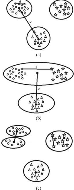
The example illustrated in Fig. 1 helps to understand these concepts. In Fig. 1a, three types of 2-dimensional samples are shown along the clustering results with suitable clusters. In Fig. 1b, a clustering result shows a big interclass distance (D) causing a smaller number of clusters and in Fig. 1c, the number of clusters increases to more than expected due to a shorter inter-class distance (D) or larger intra-inter-class distance (d).
In our study, we used Davies-Bouldin’s Index (DBi) to assess the IPO algorithm as an objective function by compromising the distance between inter-class and intra-class distances. A more detailed description of DBi is offered in the next section.
(a)
(b)
(c)
DAVIES BOULDIN INDEX
One of the most important components of an un-supervised clustering algorithm is the criterion used to determine the correct number of clusters with a proper fitness. For this reason, various validity functions and criteria have been designed to find the best number of clusters such as: Davies-Bouldin’s index (Davies and Bouldin, 1979); Fukuyama-Sugeno’s Index (Fuku-yama and Sugeno, 1989); Xie-Beni’s Index (Xie and Beni, 1991) and (Hashimoto, et al., 2009). In this paper, DBi was found most suitable and reliable for our experiments when compared to several alternative validity functions as defined in Eq. 11 and Eq. 12. The following equation calculates the intra-class diversity of the i-th cluster where Si,q is the dispersion of the
i-th cluster, and Miis its centroid; ci is the number of
points in the cluster i, and q is a constant. Therefore, if q = 2, Si,q is the standard deviation for distance in
the sample distance of a cluster with respect to the cluster centroid.
Bouldin, 1979; Chou, et al, 2004; Hashimoto, et al., 2009).
ijt
q j q i j i qt i D S S R , , ,
, max
,
(11)
K i qt i R K DB 1 ,1
.
(12)Here Ri,qt is the maximum value of DBi for i-th
cluster with respect to other clusters; t and q are the same previously mentioned constants.
IPO-CLUSTERING
q c x q i i q i i M X c S 1 2 , 1
.
(9)The interclass distance of the two clusters i and j is measured by Eq. 10 as the distance between their centroids where Mi is the centroid for i-th cluster and
t is a constant in case of t = 2. Thus, D becomes the Euclidean distance between centroids.
t j i t n k t kj ki t
ij m m M M
D d
1 1,
,
(10)The IPO algorithm context was used to solve the clustering problem and the method structure was based on two parts: 1) IPO algorithm, and 2) objective functions on DBi. A single ball in IPO (Xi)
represents kmax number of cluster centroid vectors
(M), in which each cluster center is in nd dimension.
In addition, each ball consists of a vector with kmax
random entries in the range of 0 and 1 (ri, j where i =
1, 2, …, np and j = 1, 2, …, kmax). Parameter kmax is a
limitation defined by user value for maximum number of clusters. So, balls determine which cluster centroid is active or inactive; also, it includes the specification of cluster centroids in nd dimension. To
assess which ball is active or not, a threshold is used and experimentally defined by user to determine a constant from 0 to 1 (Ti,j where i = 1, 2, …, np and j =
1, 2, …, kmax). Fig. 2 illustrates an estimation of a
single ball. If ri,j is bigger than threshold Ti,j, Mi,j in nd
dimension, it is considered as an active cluster centroid; otherwise, it is an inactive cluster.
where Mi= (m1i, m2i,...,mndi).
With these two measures, DBi appropriately calculates the closeness of the two clusters by Eq. 11, as the sum of their standard deviations is divided by the distance of their centroids. So DBi can be defined in Eq. 12 where small values of DBi show that clusters are well separated. Thus, IPO algorithm tends to reach the minimum value of DBi for the best result. Note that in Eq. 11, the worst separation of the clusters in each time iterations is selected by maximizing the value of DBi from each two clusters (worst case) in order to guarantee the best results for IPO algorithm. In the next section our proposed method of unsuper-vised IPO clustering is further explained (Davies and
Fig. 2. Shape of a ball in IPO algorithm.
For better understanding, assume that a ball has 5 cluster centroids for the maximum number of cluster limitation and it is in 3 dimensional spaces as shown in Table 1. For a threshold of 0.5, only the second, third and fifth cluster centroids are active.
After assigning this structure to the balls in IPO method, K-Nearest Neighbor (KNN) method is applied to find clusters by using the number of clusters and their centroid positions as specified by balls. Datasets
Table 1. Example for a ball in IPO method.
are searched by KNN and clusters are determined. Afterwards, DBi is calculated for clusters, and its value is used as a fitness for IPO algorithm. By time iterations, IPO algorithm tends to reach a minimum value for DBi as an objective function. So, as time passes, the best cluster centroids are stored. This process continues until the termination criteria occur. The best ball obtained from the proposed method will hold the best cluster's number and center position.
EXPERIMENTAL RESULTS
To evaluate performance of the proposed method, we have used 4 well-known standard benchmarks and tested the IPO algorithm on 3 standard images. To compare data clustering results, three other algorithm results were used such as Particle Swarm Optimi-zation (PSO), Gravitational Search Algorithm (GSA) by Rashedi et al. (2009) and Central Force Optimi-zation (CFO). Also, Image histogram clustering results were compared with those of two other methods such as Genetic Clustering with Undefined K (GCUK) (Bandyopadhyay and Maulik, 2002) and Variable Length Improved Genetic Algorithm (VLIGA) (Katari and Satapathy, 2007).
To illustrate and discuss the results of our experi-ment, we have prepared the following two subsections. At first data clustering results are explained, and then clustering method results on image histogram are shown.
IPO DATA CLUSTERING RESULTS
A standard dataset consisting of 4 famous data are listed below:
1. Iris: this is perhaps the most famous dataset in literature and in the field of clustering. The iris dataset consists of 150 instances with four numeric features, which contains three classes of 50 instan-ces, where each class refers to a type of iris plant (Bache and Lichman, 2013).
2. Wine: there are 178 instances in the wine dataset, characterized by 13 numeric features. The features are explained in the chemical analysis of three types of wine. There are also, three categories of data: 59 objects in class 1, 71 objects in class 2, and 48 objects in class 3 (Bache and Lichman, 2013).
3. Wisconsin Breast Cancer: In this dataset there are 683 instances with 9 numeric features consisting of 444 objects in class 1 (malignant) and 239 objects in class 2 (benign) (Bache and Lichman, 2013).
4. Contraceptive Method Choice (CMC): this data-set consists of 1473 samples, including 3 classes
where samples are characterized by 9 features. There are 629 instances in class 1; 334 instances in class 2 and 510 instances in class 3 (Bache and Lichman, 2013).
The problem setup for all algorithms is the same with a threshold of 0.6, where each algorithm runs 20 times. For IPO, parameters are C1 = C2 = 1, Shift1 =
Shift2 = 100, Scale1 = Scale2 = 0.002, and each
algo-rithm runs for 100 iteration. For GSA, Gamma and Alpha are 1 and 2 respectively and for CFO algo-rithm, parameters are: Gamma = 2, Alpha = 2, Beta = 2, Frepinit = 0.5, DeltaFrep = 0.1 and MinFrep = 0.05. PSO parameters are C1 = C2 = 2. It should be noted
that all of the parameters are at default values for each algorithm and no optimization process performs to find better parameters and agents in each algorithm with the same structure like balls in IPO. A compa-rison study for these 4 methods is illustrated in Table 2, showing the results are at best optimum points in 20 times run. The number of times for each algorithm was found to be the true answer (the number of clus-ters). However, this was not the optimum value of objective functions as shown in Table 3.
In Table 2, IPO clustering method from each dataset shows better results compared to the three other methods with an exception of cancer data where none of the algorithms reaches the best number of clusters. In Wine data, PSO has a better fitness but reaches a wrong cluster number. In terms of the average results, PSO, as seen in Table 3, has better results compared to IPO method in Iris and Wine data. In Table 3, the proposed method shows better results for Wine and CMC data with respect to the number of times used to reach a true cluster number. As the final analysis, we can assert that, in Table 3, the IPO method has a slight change around the best results, and diversity is smaller than other algorithms, especially in CMC data.
The time and speed of problem solving are also good criteria to compare these methods. In Table 4, the speed of each method on Iris data is illustrated in seconds and compared the number of particles used in calculation (Neval).
Table 2. Result comparison for the optimum value of objective function and cluster number.
Minimum of objective function DB index Number of optimum cluster centroids IPO CFO PSO GSA IPO CFO PSO GSA Iris 0.2173 0.4367 0.2560 0.3288 3 2 3 6
Wine 0.1798 0.298 0.1508 0.1848 3 5 4 6 Cancer 0.5982 1.2687 0.7108 0.8943 3 4 3 10 CMC 0.3338 0.6351 0.3472 0.3732 3 5 3 4 Table 3. Result comparison for the number of times each method reaches the true answer.
Times of the true cluster
number in 20 runs Average of 20 runs Standard deviation of results in 20 runs IPO CFO PSO GSA IPO CFO PSO GSA IPO CFO PSO GSA Iris 11 9 15 0 3.6 3.6 3.5 5.15 0.7539 0.8208 0.9459 1.0894 Wine 5 3 3 0 4.3 5.25 4.15 7.4 1.5252 2.2213 2.3681 2.0876 Cancer 6 7 3 0 3.7 3.3 3.35 7.75 1.9494 1.3803 1.2680 2.3814 CMC 15 10 13 0 3.2 3.55 3.5 5.9 0.6156 0.8256 0.7609 1.8035 Table 4. Method comparison in terms of problem solving speed.
Algorithm methods
Amount of time for solving
in second Neval
Number of cluster in this run
Objective function value in this run
IPO 12.1262 4000 3 0.3316
CFO 63.0232 4040 4 0.4304
GSA 12.4574 4000 3 0.4744
PSO 22.1909 8040 3 0.2834
Table 5. The results of clustering methods on standard images.
IMAGE VLIGA GCUK IPO-Clustering
DB 0.5203 ± 0.0120 0.5309 ± 0.032 0.2237 ± 0.0382
LENA
K 5-7 4-8 4-8
DB 0.4262 ± 0.011 0.4623 ± 0.0019 0.3331 ±0.0447
CAMERAMAN
K 4-6 3-6 3-7
DB 0.5292 ±0.034 0.5343 ±0.025 0.2432 ±0.0326
PEPPER
K 4-8 4-9 4-8
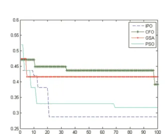
Fig. 3. Study comparison for the best fitness (x axis: iteration, y axis: fitness).
IPO IMAGE HISTOGRAM CLUSTERING
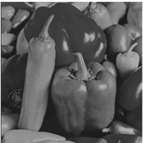
Figs. 4–9 illustrate three standard grayscale images with their histograms. The comparison results of three methods on standard images are shown in Table 5. The parameters of IPO remain the same as seen in previous section. The IPO and two other methods were tested 20 times on each image histogram.
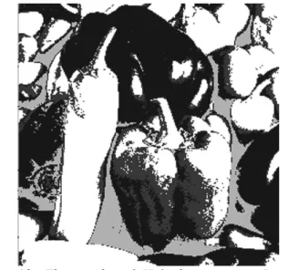
After clustering image histograms, images are clustered by using histogram threshold by values of cluster centroids. As we can see in Table 5, IPO has a better result for value of objective function in all cases. IPO method can find the number of cluster centroids in near optimum range in comparison to VLIGA and GCUK methods. So, in terms of fitness, the IPO clustering has offered significantly better results than the two other methods. In Figs. 10–12, the illustrated image results reveal a fine clustering by using the IPO method.
Fig. 4. Image, Lena with 512×512 dimensions.
Fig. 5. Histogram of image, Lena.
Fig. 6. Image, Peppers with 512×512 dimensions.
Fig. 7. Histogram of image, Peppers.
Fig. 9. Histogram of image, Cameraman.
Fig. 10. The results of IPO-clustering on Lena image.
Fig. 11. The results of IPO-clustering on Cameraman image.
Fig. 12. The results of IPO-clustering on Peppers image.
CONCLUSION
This study investigated the application of Inclined Planes system Optimization algorithm on data clustering and grayscale histogram images. Hybrid of IPO algorithm, DBi and KNN method were combined to find optimum number of clusters in available data. Several famous data benchmarks and few standard image datasets were used to illustrate the proposed method results. Histogram of images was used to reduce the amount of the data and increase the calculation speed. In terms of data clustering, the proposed IPO method was compared with other well-known methods. Four optimization algorithms were used in terms of image clustering and the results of 2 similar image clustering methods were compared with the proposed IPO method. In conclusion, researchers found the results of IPO method compared with other similar methods were more powerful in most cases.
ACKNOWLEDGEMENTS
The authors would like to thank Dr. Marjaneh M. Fooladi, Mr. Ali Pourvali and Mr. Hamed Abdi for their valuable editorial assistance.
REFERENCES
Bandyopadhyay S, Maulik U (2002). Genetic clustering for automatic evolution of clusters and application to image classification. IEEE Pattern Recogn 35:1197–208. Chou C, Su M, Lai E (2004). A new cluster validity measure
and its application to image compression. Pattern Anal Appl 7:205–20.
Davies DL, Bouldin DW (1979). A cluster sparation measure. IEEE T Pattern Anal Machine Intell PAMI-1:224–7. De Souza JG, Costa JAF (2009). Unsupervised data clustering
and image segmentation using natural computing tech-niques. IEEE Sys Man Cybern 5045:11–4.
Dembele D (2008). Multi-objective optimization for clus-tering 3-way gene expression data. Adv in Data Anal Class 2:211–25.
Dimitriadou E, Dolnicar S, Weingassel A (2002). An exami-nation of indexes for determining the number of clusters in binary data sets. Psychometrika 67:137–59.
Dorigo M (1992). Optimization, learning and netural algo-rithms. PhD Thesis, Politecnio di Milano, Italy.
Farmer J, Packard N, Perelson A (1986). The immune system, adaptation, and machine learning. Physica D Arch 2: 187–204.
Formato R (2007). Central force optimization: a new meta-heuristic with applications in applied electromagnetics. Prog Electromagn Res 77:425–91.
Fukuyama Y, Sugeno M (1989). A new method of choosing the number of clusters for the fuzzy c-means method. Proceeding of fifth Fuzzy Syst Symp, pp. 247–50. Garcia-Escudero L, Gordaliza A, Matran C (2010). A review
of robust clustering methods. Advances in Data Analysis and Classification 4:89–109.
Geem Z, Kim J, Loganathan G (2001). A new heuristic opti-mization algorithm: Harmony search. Simulation 76:60–8. Hashimoto W, Nakamura T, Miyamoto S (2009). Comparison and evaluation of different cluster validity measures in-cluding their kernelization. J Adv Comput Intell Inform 13:204–9.
Jain AK, Murty MN, Flynn PJ (1999). Data clustering: a review. ACM Comput Surv, ACM Press 31:264–323. Katari V, Satapathy S (2007). Hybridized improved genetic
algorithm with variable length chromosome for image clustering. IJCSNS Int J Comput Sci and Netw Sec 7: 121–31.
Kennedy J, Eberhart R (1995). Particle swarm optimization. Proceedings of the IEEE Int Conf Neural Networks 4: 1942–8.
Krikpatrick S, Gelatt CD, Vecchi MP (1983). Optimization by simulated annealing. Science 220:671–80.
Lezoray O (2011). Supervised automatic histogram clustering and watershed segmentation. Application to microscopic medical color images. Image Anal Stereol 22:113–20. Maulik U, Bandyopadhyay S (2000). Genetic
algorithm-based clustering technique. J Pattern Recogn 33:1455–65. Mozaffari MH, Abdy H, Zahiri SH (2013). Application of
inclined planes system optimization on data clustering. Pattern Recogn and Image Anal (PRIA), First Iranian Conference, 1:6–8.
Omran GH, Engelbrecht AP, Salman A (2005). Dynamic clustering using particle swarm optimization with application in unsupervised image classification. Trans Eng Comput Tech 9:199–204.
Rashedi E, Nezamabadi-pour H, Saryazdi S (2009). GSA: A gravitational search algorithm. Inform Sciences 179: 2232–48.
Sang CS (2012). Practical application of DATA MINING. USA: Texas A&M University, Jones and Bartlett. Tang KS, Man KF, Kwong S, He Q (1996). Genetic
algo-rithms and their applications. IEEE Signal Proc Mag 13:22–37.
Tseng L, Yang S (2001). A genetic approach to the automatic clustering problem. Pattern Recogn 34:415–24.
Wataru H, Tetsuya N, Sadaaki M (2009). Comparison and evaluation of different cluster validity measures including their kernelization. J Adv Comput Intell and Intell Info 13:204–9.
Xie XL, Beni G (1991). A validity measure for fuzzy clus-tering. IEEE T Pattern Anal Machine Intelli 3:841–6. Xu R, Wunsch II D (2005). Survey of clustering algorithms.
IEEE T Neural Networks 16:645–78.
Xu R, Wunsch II D (2008). Clustering. Wiley-IEEE. Yamamoto M (2012). Clustering of functional data in a
low-dimensional subspace. Adv Data Anal Classif 6: 219–47.