SPATIALLY ADAPTIVE MORPHOLOGICAL IMAGE FILTERING
USING INTRINSIC STRUCTURING ELEMENTS
JOHAN
DEBAYLE AND
JEAN-CHARLES
PINOLI
´Ecole Nationale Sup´erieure des Mines de Saint-Etienne, 158, cours Fauriel Saint- ´Etienne cedex 2, France e-mail: [email protected], [email protected]
(Accepted October 21, 2005)
ABSTRACT
This paper deals with spatially adaptive morphological filtering, extending the theory of mathematical morphology to the paradigm of adaptive neighborhood. The basic idea in this approach is to substitute the extrinsically-defined, fixed-shape, fixed-size structuring elements generally used by morphological operators, by intrinsically-defined, variable-shape, variable-size structuring elements. These last so-called intrinsic structuring elements fit to the local features of the image, with respect to a selected analyzing criterion such as luminance, contrast, thickness, curvature or orientation. The resulting spatially-variant morphological operators perform efficient image processing, without any a priori knowledge of the studied image and some of which satisfy multiscale properties. Moreover, in a lot of practical cases, the elementary adaptive morphological operators are connected, which is topologically relevant. The proposed approach is practically illustrated in several application examples, such as morphological multiscale decomposition, morphological hierarchical segmentation and boundary detection.
Keywords: adaptive neighborhood, connected operators, intrinsic spatial analysis, mathematical morphology, multiscale representation.
INTRODUCTION
Firstly, a lot of image processing techniques use spatially-invariant transformations, with fixed operational windows. This kind of operators, such as morphological operators or convolution filters, give efficient and compact computing structures, in the sense where data and operators are independent. However, due to their fixed operational windows, they consequently have several strong drawbacks such as creating artificial patterns, changing the detailed parts of large objects, damaging transitions or removing significant details (Arce and Foster, 1989).
Alternative approaches towards spatially-variant
image processing have been proposed (Gordon and Rangayyan, 1984; Perona and Malik, 1990; Salembier, 1992; Alvarez et al., 1993; Charif-Chefchaouni and Schonfeld, 1994; Vogt, 1994; Braga Neto, 1996; Cuisenaire, 2005; Lerallut et al., 2005) with the introduction of adaptive operators, where the adaptive concept results from the spatial adjustment of the operational window. A spatially adaptive operator will no longer be spatially-invariant, but must vary over the whole image with adaptive windows, taking locally into account the image context. Such transforms perform efficient image processing.
Secondly, usual image processing operators have some limitations concerning their operational windows (adaptive or not). In fact, these last ones are usually
extrinsicallydefined with regard to the local features
of the image. A priori constraints are imposed upon the size and/or the shape of the operational windows, which is not the most appropriate. For instance, spatially-invariant approaches such as wavelets (Mallat, 1989), morphological pyramids (Sun and Maragos, 1989; Laporterie et al., 2002), and isotropic scale-spaces (Lindeberg, 1994; Heijmans and Boomgaard, 2000) use sliding windows extrinsically defined with regard to the analyzing scales. Indeed, their size and shape are fixed on the whole image for each scale, i.e., a priori determined, independently of the image context. In an other example (Vogt, 1994), spatially-variant morphological operators are used, where the shape of morphological structuring elements that automatically adjust the gray tones in a range image is rectangular or ellipsoidal, involving a priori knowledge about the image context.
perform meaningful image processing as shown in various image filtering processes (Rabieet al., 1994; Rangayyan et al., 1998; Rangayyan and Das, 1998; Ciucet al., 2000; Buzuloiuet al., 2001; Ciuc, 2002).
In this paper, an intrinsic spatially-variant approach in the context of Mathematical Morphology (MM) is then proposed using autoreflected Structuring Elements (traditionally called symmetric (Serra, 1988a), i.e., structuring elements which are equal to their reflected set), based on the AN paradigm.
While autoreflectedness is not necessary in the general framework of spatially-variant mathematical morphology, as formally proposed by Charif-Chefchaouni and Schonfeld (1994) and practically used by Cuisenaire (2005) and Lerallutet al.(2005), it is relevant for three main reasons:
1. it is more adapted to image analysis for topological and visual reasons,
2. both dualities by adjunction and by involution for dilation and erosion are satisfied,
3. it allows to simplify mathematical expressions of morphological operators, without increasing computational complexity of algorithms.
Thereafter, the fixed-size, fixed-shape SEs generally used for morphological operators are substituted by (intrinsic) Adaptive Structuring Elements (ASEs) adjusted to a specified set of adaptive neighborhoods based on an analyzing criterion. It leads to Adaptive Neighborhood Mathematical Morphology (ANMM), which provides convincing spatially adaptive morphological filters (Debayle and Pinoli, 2005a). Some of which satisfy multiscale properties (Debayle and Pinoli, 2005b). Moreover, in a lot of practical cases, the elementary adaptive morphological operators are connected, contrary to the usual ones which fail to this property. The proposed approach is practically illustrated through several application examples, such as multiscale decomposition, hierarchical segmentation and boundary detection on the ‘cameraman’ image, the ‘tools’ image and a metallurgic grains real image, respectively.
ADAPTIVE NEIGHBORHOOD
SETS
The first step in this ANMM approach consists in defining a set of adaptive neighborhoods determined on the spatial support of the studied image.
Let D⊆R2 (or more generally in Rn (Debayle,
2005)), the (usually rectangular) domain of definition
of the images and I the set of image mappings from D into R. For each point x ∈D of an image f ∈I, the adaptive neighborhood (AN) sets, denoted
Vh
m(x), are computed in relation with an homogeneity tolerance m ∈R+ on a criterion mapping h (based
on a local measurement such as luminance, contrast, curvature, thickness or orientation related to the image
f) belonging to the setCof mappings fromDintoR.
More precisely, for all pointx∈Dits associated AN setVh
m(x)⊆D:
• depends on two parameters: - h: analyzing criterion - m: homogeneity tolerance • fulfills two conditions:
- its points have a measurement value close to that of the pointx:
∀y∈Vmh(x) |h(y)−h(x)| ≤m
- the set is path-connected (with the usual Euclidean topology onD⊆R2)
Definition 1 (AN sets) ∀(m,h,x)∈R+×C×D
Vmh(x) = Ch−1([h(x)−m,h(x)+m])(x), (1)
where CX(x) denotes the path-connected component (with the usual Euclidean topology on D ⊆R2) of X⊆Dcontainingx∈D.
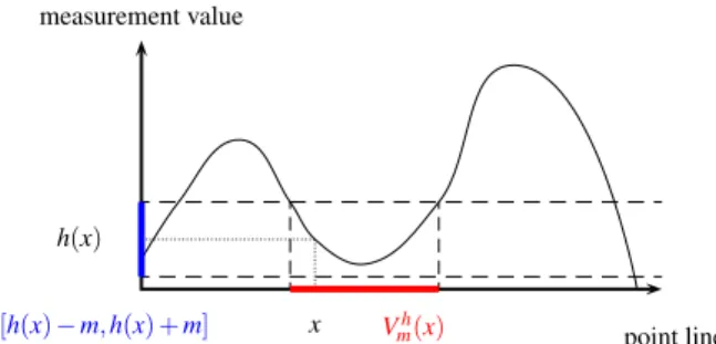
Fig. 1 gives an impression, on a 1-D example, of the computation of an AN set.
point line measurement value
x h(x)
[h(x)−m,h(x) +m] Vh
m(x)
Fig. 1. One-dimensional computation of an adaptive neighborhood set Vh
m(x). For a point x, a tube of
tolerance m is first computed around h(x). Secondly,
the inverse image of this interval gives a subset of the 1-D spatial support. Finally, the path-connected component holding x provides its AN set Vh
m(x).
criterion, on an electrophoresis gel image provided by the software Micromorph°R. In practice, the choice of the appropriate criterion results from kind of the considered application.
(a) original image (b)h1: luminance
(c)h2: contrast (d) seed pointx
(e)Vh1
10(x) (f)V30h2(x)
Fig. 2. Original electrophoresis gel image (a). The adaptive neighborhood set for the seed point highlighted in (d) is respectively homogeneous (e,f), with respect to the tolerance m, in relation to the luminance criterion (b) or to the contrast criterion (c).
In the following, the notion of path is defined so as to get a practical equivalent definition of these AN sets, involving computing interests.
Definition 2 (Path)
A path of extremities x∈D and y ∈D respectively, denoted Pyx, is a continuous mapping (with the usual Euclidean topologies on[0,1]andD) (Choquet, 2000):
Pyx:
[0,1] → D
0 7→ x
1 7→ y . (2)
So, the AN sets Vh
m(x)are defined with the help of a region growing process, which is of great computing importance, where the aggregating condition is given by:|h(.)−h(x)| ≤m.
Definition 3 (AN sets - equivalent definition) ∀(m,h,x)∈R+×C×D
Vhm(x) = {y∈D|y−→h,m x}, (3)
where−→h,m denotes the path-connectivity relationship:
y−→h,m x ⇔ ∃Pyx|∀z∈Pyx([0,1])|h(z)−h(x)| ≤m.
Remark 1 This definition of the AN sets Vh m(x) is similar to those of connected regionsRmf(x)defined by Braga Neto (1996) but are more general in the sense that they take into account a criterion mappingh.
These AN sets satisfy several properties as stated in the following:
Properties 1 (AN sets) Let(m,h,x)∈R+×C×D
1. reflexivity:
x∈Vhm(x) (4)
2. increasing with respect tom:
µ
(m1,m2)∈R+2 m1≤m2
⇒Vhm1(x)⊆Vhm2(x) (5)
3. equality between iso-valued points:
(x,y)∈D
2
x∈Vhm(y)
h(x) =h(y)
⇒Vhm(x) =Vhm(y) (6)
4. addition invariance with respect toh:
c∈R⇒Vhm+c(x) =Vhm(x) (7)
5. multiplication compatibility with respect toh:
α∈R+\{0} ⇒Vmαh(x) =Vhm
α(x) (8)
Proof:
2.
m1≤m2 ⇒ [h(x)−m1,h(x)+m1]⊆
[h(x)−m2,h(x) +m2])
⇒ Ch−1([h(x)−m1,h(x)+m1])(x)⊆
Ch−1([h(x)−m2,h(x)+m2])(x) ⇒ Vhm1(x)⊆Vhm2(x)
3. Letzbe a point in Vhm(x). So, there exists a path Pzx such that:∀w∈Pzx([0,1])|h(w)−h(x)| ≤m. Moreover,x belongs to Vh
m(y), i.e., there exists a path Px
ysuch that:
∀u∈Pxy([0,1])|h(u)−h(y)| ≤m. Thus, there exists a path Pz
y such that Pzy([0,1]) = Pxy([0,1])∪Pzx([0,1]).
Consequently, for alltin Pz
y([0,1]), ift belongs to Pxy([0,1])then |h(t)−h(y)| ≤m elset belongs to Pzx([0,1])and|h(t)−h(y)|=|h(t)−h(x)| ≤m. So, for allt in Pz
y([0,1])|h(t)−h(y)| ≤mand then
z∈Vhm(y).
Conversely, ifzbelongs to Vh
m(y)then there exists a path Pz
ysuch that:
∀w∈Pzy([0,1])|h(w)−h(y)| ≤m. Since x belongs to Vh
m(y) and h(y) =h(x), then
y belongs to Vh
m(x) (seen with the inverse path Pyx(.) =Pbxy(.) =Pxy(1−.)).
So, there exists a path Pz
x such that Pzx([0,1]) = Pyx([0,1])∪Pzy([0,1]).
A similar reasoning leads to the expecting result,
i.e.,z∈Vhm(x).
4. (h+c)−1([(h+c)(x)−m,(h+c)(x)+m]) ={y∈D|(h+c)(y)∈[(h+c)(x)−m,
(h+c)(x) +m]} ={y∈D|h(y)∈[h(x)−m,h(x)+m]} =h−1([h(x)−m,h(x)+m])
5. (αh)−1([(αh)(x)−m,(αh)(x) +m])
={y∈D|(αh)(y)∈[(αh)(x)−m,(αh)(x)+m]} ={y∈D|h(y)∈[h(x)−(mα),h(x) + (mα)]} =h−1([h(x)−(m
α),h(x) + (mα)])
¤
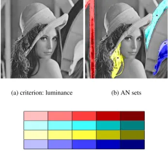
To illustrate the nesting property (Eq. 5) with respect to m, the AN sets of four initial points are computed on the ‘Lena’ image (Fig. 3) with the luminance as analyzing criterion.
(a) criterion: luminance (b) AN sets
m=5
m=10
m=15
m=20
m=25
(c) color table
Fig. 3.Nesting of AN sets of four seed points (b) using the luminance criterion (a) and different homogeneity tolerances: m=5,10,15,20 and 25 encoded by the color table (c). An AN set defined with a certain homogeneity tolerance could be represented by several tinges of the color associated to its seed point.
Fig. 3 shows that the AN sets are, through the analyzing criterion and the homogeneity tolerance, intrinsically-defined with respect to the local structures of the studied image, performing a real spatially adaptive analysis.
So, morphological operations have to be adjusted to these AN sets so as to develop Adaptive Neighborhood Mathematical Morphology (ANMM).
tools in the aim of image filtering, image segmentation and classification, image measurements, pattern recognition, or texture analysis.
Inspired by Braga Neto (1996), the proposed spatially-variant mathematical morphology approach is based on the adaptive neighborhood paradigm proposed by Paranjapeet al.(1994). In this paper, only the flat MM (ie with structuring elements as subsets in
R2) is considered, though the approach is not restricted
and can also address the general case of functional MM (ie with functional structuring elements from a subset ofDintoR) (Debayle, 2005).
The space of imagesI is provided with the partial ordering relation ≤ defined in terms of the usual ordering relation≤of real numbers:
∀(f,g)∈I f≤g⇔(∀x∈D f(x)≤g(x)). (9)
Thus, the partially-ordered set(I,≤), still namedI, is a complete lattice (Serra, 1988a).
ADAPTIVE STRUCTURING ELEMENTS
To get the morphological duality (adjunction) between erosion and dilation, reflected (or transposed) structuring elements (SEs) (Serra, 1988a), whose definition is mentioned below, should be used.
Definition 4 (Reflected subset) The reflected subset of A(x)⊆ D, element of a collection {A(z)}z∈D, is defined as:
ˇ
A(x) ={z∈D;x∈A(z)}. (10)
The notion of autoreflectedness is then defined as following (Serra, 1988a):
Definition 5 (Autoreflected subset) The subset
A(x) ⊆ D, element of a collection {A(z)}z∈D is autoreflected if and only if:
ˇ
A(x) =A(x), (11)
that is to say:∀(x,y)∈D2 x∈A(y)⇔y∈A(x).
Remark 2 The term autoreflectedness is employed in place of symmetry which is generally used in literature (Serra, 1988a), so as to avoid the confusion with the geometrical symmetry. Indeed, an autoreflected subset
A(x) ⊆ D belonging to {A(z)}z∈D is generally not symmetric with respect to the pointx.
Spatially-variant mathematical morphology using adaptive SEs which do not satisfy the autoreflectedness condition (Eq. 11) has been formally proposed
by Charif-Chefchaouni and Schonfeld (1994) and practically used in image processing (Lerallut
et al., 2005; Cuisenaire, 2005). Nevertheless, while autoreflectedness is restrictive from a strict mathematical point of view, it is relevant for three main reasons:
1. it is more adapted to image analysis for topological and visual reasons (Rem. 3),
2. both dualities by adjunction and by involution for dilation and erosion are satisfied,
3. it allows to simplify mathematical expressions of morphological operators, without increasing computational complexity of algorithms.
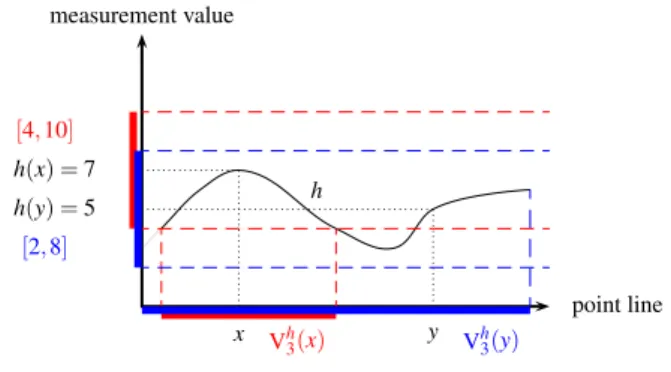
From this point, autoreflected adaptive structuring elements are considered in this paper. Therefore, the AN setsVh
m(x)are not autoreflected (Fig. 4).
point line measurement value
x h(x) =7
y h(y) =5 h
[4,10]
[2,8]
Vh
3(x) Vh3(y)
Fig. 4.The AN sets{Vhm(z)}z∈Dare not autoreflected:
x∈Vh3(y)and y∈/Vh3(x). Consequently,(Vˇh3)6=Vh3.
So, the adaptive SEs, denoted {Rh
m(x)}x∈D, are defined while satisfying the AN paradigm and the autoreflectedness condition.
Definition 6 (Adaptive structuring elements) ∀(m,h,x)∈R+×C×D
Rhm(x) = [ z∈D
{Vmh(z)|x∈Vmh(z)}. (12)
These adaptive SEs (Eq. 12) are anisotropic and self-defined with respect to the criterion image mappingh. They satisfy the following properties:
Properties 2 (Adaptive structuring elements) ∀(m,m1,m2,h,x)∈R+3×C×D
1. geometric nesting:
Vhm(x)⊆Rhm(x)⊆Vh2m(x) (13)
2. symmetry:
3. reflexivity:
x∈Rhm(x) (15)
4. increasing with respect tom:
m1≤m2⇒Rhm1(x)⊆Rhm2(x) (16)
5. addition invariance with respect toh:
c∈R⇒Rhm+c(x) =Rhm(x) (17)
6. multiplication compatibility with respect toh:
α∈R+\{0} ⇒Rmαh(x) =Rhm
α(x) (18)
Proof:
1. Since x belongs to Vh
m(x), Vhm(x) is included as subset inRh
m(x). Lety be a point in Rh
m(x). So, there exists z inD such thatybelongs to Vh
m(z)(with the path Pyz) and
xbelongs to Vh
m(z)(with the path Pxz).
Thus, the path Pyxsuch that Pyx([0,1]) =Pˇxz([0,1])∪ Pyz([0,1])is well-defined.
Let w in Pyx([0,1]). If w belongs to Pyz([0,1]) then |h(w)−h(x)| ≤ |h(w)−h(z)|+|h(z)−h(x)| ≤
m+m = 2m, else w belongs to ˇPx
z([0,1]) = Pxz([0,1]) ( ˇPxz and Pxz have same image) and so |h(w)−h(x)| ≤ |h(w)−h(z)|+|h(z)−h(x)| ≤
m+m=2m. Consequently,∀w∈Pyx([0,1]) |h(w)−h(x)| ≤2mand thereforey∈Vh2m(x).
2. Ifybelongs toRh
m(x), there existszinDsuch that
yandxboth belong to Vh
m(z). So,Rhm(y)holdsx. 3-6.These properties are inferred from the
corresponding ones of AN sets (Prop. 1).
¤
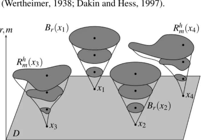
The ASEs satisfy the AN paradigm through the geometric nesting (Eq. 13). Fig. 5 compares the shape of usual SEs Br(x) as disks of radius r ∈R+ and adaptive SEsRh
m(x)as sets self-defined with respect to the criterion mappinghand the homogeneity tolerance
m∈E+.
Remark 3 Autorefletedness is argued to be more
adapted to image analysis from both topological and visual reasons. In fact, it allows a symmetric neighborhood systemRh
m(x)to be defined at each point
xbelonging to D. Topologically, it means that ifxis in the neighborhood ofy at levelm (x∈Rhm(y)), then y is as close to x as x is close to y (y∈Rh
m(x)) (Prop 2.2). In terms of metric, this is a required condition to define a distance function d, starting from all the
Rh
m(.), satisfying the symmetry axiom:d(x,y) =d(y,x)
(Cech, 1966). Indeed, symmetry is needed to introduce a non-degenerate topological metric space (the authors are currently working on topological approaches with respect to the AN paradigm). From a visual point of view, the symmetry property appears closely linked to the human visual perception (Gestalt theory, . . . ) (Wertheimer, 1938; Dakin and Hess, 1997).
D
x1
Br(x1)
x
2
Br(x2)
x 3 Rh m(x3)
x
4
Rh m(x4)
r,m
Fig. 5.Example of adaptive Rh
m and non-adaptive Br
structuring elements with three values both for the homogeneity tolerance parameter m, and for the disks radius r. The shape of Br(x1)and Br(x2)are identical
and{Br(x)}r is a family of homothetic sets for each
point x∈D. On the contrary, the shape of Rhm(x3)and
Rh
m(x4)are dissimilar and{Rm(x)}mis not a family of
homothetic sets.
The next step consists in defining adaptive basic operators of MM in the aim of building adaptive morphological filters.
ADAPTIVE ELEMENTARY
MORPHOLOGICAL OPERATORS
The elementary dual operators of adaptive dilation and erosion are defined accordingly to the flat ASEs
Rh
m(x). The formal definitions are given as following:
Definition 7 (Adaptive dilation/erosion) ∀(m,h)∈R+×C
Dhm :
½ I
→ I
f 7→ Dhm(f) , (19)
where Dhm(f) :
( D → R x 7→ sup
w∈Rhm(x)f(w) (20)
Ehm :
½ I
→ I
f 7→ Ehm(f) , (21)
where Ehm(f) :
(
D → R x 7→ inf
w∈Rh m(x)
Next, the lattice theory (Serra, 1988a) allows to define the most elementary (adaptive) morphological filters (Serra, 1988b). More precisely, the adaptive closing and opening are respectively defined as:
Definition 8 (Adaptive closing/opening) ∀(m,h)∈R+×C
Chm :
½ I
→ I
f 7→ Ehm◦Dhm(f) , (23)
Ohm :
½
I → I
f 7→ Dhm◦Ehm(f) . (24)
These adaptive elementary morphological operators satisfy several properties stated in the following. Properties 1 through 6 are standard, that is to say analogous to those of the usual morphological operators:
Properties 3 (Adaptive morphological operators) Let(m,h,f,f1,f2)∈R+×C×I3.
1. increasing:
f1≤f2⇒
Dhm(f1)≤Dhm(f2)
Ehm(f1)≤Ehm(f2)
Chm(f1)≤Chm(f2)
Ohm(f1)≤Ohm(f2)
(25)
2. adjunction (morphological duality):
Dhm(f1)≤ f2⇔ f1≤Ehm(f2) (26)
3. extensiveness, anti-extensiveness:
Ohm(f)≤ f ≤Chm(f) (27)
4. distributivity withW,V:
∀(fi)∈IK
_ i∈K
[Dhm(fi)] =Dhm(_ i∈K
[fi])
^
i∈K
[Ehm(fi)] =Ehm(
^
i∈K
[fi]) (28)
whereKis an index set (finite or not). 5. duality with respect to the involution ¯.:
(
Dhm(f) =Ehm(f) Ch
m(f) =Ohm(f)
(29)
6. idempotence:
½
Chm(Chm(f)) =Chm(f)
Ohm(Ohm(f)) =Ohm(f) (30)
7. increasing, decreasing with respect tom:
µ
(m1,m2)∈R+2 m1≤m2
⇒
½
Dhm1(f)≤Dhm2(f) Ehm1(f)≥Ehm2(f)
(31) 8. addition invariance with respect toh:
c∈R⇒
Dh+c
m (f) =Dhm(f) Eh+c
m (f) =Ehm(f) Ch+c
m (f) =Chm(f) Oh+c
m (f) =Ohm(f)
(32)
9. multiplication compatibility with respect toh:
α∈R+\{0} ⇒
Dαmh(f) =Dhm α(f)
Eαmh(f) =Ehm α(f)
Cαmh(f) =Chm α(f)
Oαmh(f) =Ohm α(f)
(33)
Proof:
1-6.These properties are inferred from the lattice theory of increasing mappings (Serra, 1988a;b). 7-9.It is directly inferred from the properties 4-6 of the
adaptive structuring elements (Prop. 2).
¤
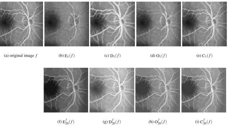
The usual and adaptive morphological operators of erosion, dilation, opening and closing are illustrated in Fig. 6. Note that Er, Dr, Orand Crdenote the classical erosion, dilation, opening, closing with the disk Br of radiusras isotropic structuring element.
Moreover, with the ‘luminance’ criterion (h=f), the adaptive dilation (Eqs. 19-20) and erosion (Eqs. 21-22) satisfy the connectedness (Serra and Salembier, 1993) condition (Prop. 4) which is of great morphological importance. On the contrary, the usual dilation and erosion fail to this property.
Definition 9 (Connectedness) An operator φ :I 7→I is connected if and only if:
∀f∈I ∀(x,y)neighbors
f(x) = f(y)⇒φ(f)(x) =φ(f)(y). (34)
Properties 4 (Connectedness of adaptive operators)
∀m∈R+ (
f7→Dmf(f)
(a) original image f (b) E1(f) (c) D1(f) (d) O1(f) (e) C1(f)
(f) E20f (f) (g) D20f (f) (h) O20f (f) (i) C20f (f)
Fig. 6.Usual vs adaptive morphological operators on a blood vessels (a) image f : usual erosion (b) / dilation (c) / opening (d) / closing (e) with a disk of radius1as isotropic SE - adaptive erosion (f) / dilation (g) /opening (h) / closing (i) with adaptive SE computed with the luminance criterion f and the homogeneity tolerance m=20.
Proof:
Let g be in I. For all (x,y) neighboring points (with the usual Euclidean topology on D⊆R2), if g(x) = g(y) then Vmg(x) =Vmg(y). In addition, for all z∈D,
x∈Vmg(z)⇒y∈Vmg(z)sincexandyare neighbors with the same gray tone.So,Rgm(x) =Rgm(y). Consequently,
Dgm(g)(x) =Dgm(g)(y)andEmg(g)(x) =Emg(g)(y). Thereafter, the closing and the opening are connected operators by composition of connected operators
(Serra and Salembier, 1993). ¤
This property is an overwhelming advantage in comparison to the usual ones which fail to this connectedness condition. Besides, it allows to define several connected operators built by composition or combination with the supremum and the infimum (Serra and Salembier, 1993) of these adaptive elementary morphological operators, as adaptive closings (Eq. 23) and openings (Eq. 24). Thus, the operators OCh
m = OhmChm and COhm = ChmOhm, called adaptive opening-closing and adaptive closing-opening respectively, are (adaptive) morphological filters (Matheron, 1988), and in addition, connected operators with the luminance criterion.
ADAPTIVE SEQUENTIAL
MORPHOLOGICAL OPERATORS
The families of adaptive morphological filters {Ohm}m≥0(Eq. 24) and{Chm}m≥0(Eq. 23) are generally
not a size distribution and anti-size distribution respectively, due to the notion of semi-group which is generally not satisfied (Serra, 1988a). Nevertheless, such families are built by naturally reiterate adaptive dilation or erosion. Explicitly, adaptive sequential dilation, erosion, closing and opening, are respectively defined as:
Definition 10 (Adaptive sequential dilation/erosion) ∀(m,p,h)∈R+×N×C
Dhm,p :
I → I
f 7→ D|hm◦ · · · ◦{z Dhm} ptimes
(f) (35)
Ehm,p :
I → I
f 7→ Ehm◦ · · · ◦Ehm
| {z }
ptimes
(f) (36)
Chm,p :
½ I
→ I
f 7→ Ehm,p◦Dhm,p(f) , (37)
Ohm,p :
½ I
→ I
f 7→ Dhm,p◦Ehm,p(f) . (38)
The morphological duality of Dh
m,p (Eq. 33) and Ehm,p (Eq. 34) provides, so among other things, the
two sequential morphological filters Ch
m,p(Eq. 35) and Ohm,p(Eq. 36). Moreover, these last ones generate size and antisize distributions:
Properties 5 (Size/antisize distribution) ∀(m,h)∈R+×C
1. {Ohm,p}p≥0is a size distribution
2. {Chm,p}p≥0is an antisize distribution
Proof:
Let f ∈I and(p,q)∈N2such that p≥q.
Ohm,p ≤ Dhm,q◦Dmh,p−q◦Ehm,p−q◦Ehm,q ≤ Dhm,q◦Omh,p−q◦Ehm,q
≤ Dhm,q◦Ehm,q
≤ Ohm,q.
Chm,p ≥ Ehm,q◦Emh,p−q◦Dhm,p−q◦Dhm,q ≥ Ehm,q◦Cmh,p−q◦Dhm,q
≥ Ehm,q◦Dhm,q
≥ Chm,q
¤
Thus, the extension of the well-known alternating sequential filters (ASFs) (Serra, 1988c) can be defined:
Definition 12 (Adaptive alternating sequential filters) ∀(m,n,h) ∈ R+ × N\{0} × C ∀(pi) ∈ NJ1,nK
increasing sequence ASFOCh
m,n:
½ I
→ I
f 7→ OChm,pn◦ · · · ◦OChm,p1(f)(x) (39)
ASFCOhm,n:
½
I → I
f 7→ COhm,pn◦ · · · ◦COhm,p1(f)(x) (40)
These adaptive ASFs are similar to those defined by Braga Neto (1996) using the AN paradigm.
RESULTS
Adaptive morphological processes are now applied and illustrated in the field of image filtering and segmentation. The results are all achieved with the luminance criterion (mappingh).
MULTISCALE DECOMPOSITION
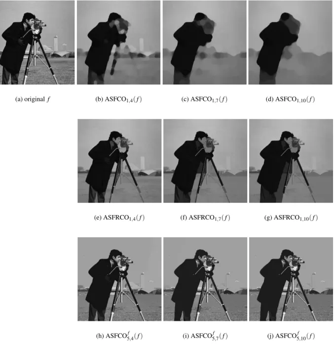
In this subsection, a multiscale representation of the ‘cameraman’ image (Fig. 7) is constituted following a specific kind of morphological operators: the alternating sequential filters (ASFs) which satisfy relevant multiscale properties (Serra and Salembier, 1993). Usual ASFs, usual ASFs by reconstruction (Crespoet al., 1995) and adaptive ASFs, are applied, supplying results which are compared and discussed.
Note that ASFCOm,p and ASFRCOm,p stand for the usual ASF and the ASF by reconstruction of order
p, respectively, with a disk of radiusmas uniform SE. As regards the filter ASFCOmf,p, it denotes the adaptive ASF of order p using the adaptive SEs with the luminance criterion mapping f and the homogeneity tolerancem.
These results show that the connectedness of adaptive ASFs and usual ASFs by reconstruction is an overwhelming advantage. Indeed, the edges are quickly damaged by the usual ASFs, while they are preserved with the connected ASFs. Moreover, the filters by reconstruction remove fine details so far, as revealed in the scene upon the camera (Fig. 7e) and the eye of the human face (Fig. 7e), although they are connected. On the contrary, the decomposition of the original image with ANMM-based filters, does not decimate relevant structures from fine-to-coarse scales (Fig. 7h-j).
BOUNDARY DETECTION
A real example in the field of image segmentation is now illustrated on a metallurgic grain boundaries image (Fig. 8). Several methods have ever been introduced (e.g., Chazallon and Pinoli, 1997) requiring most of the time complex processes. Elementary ANMM-based processing is then suggested and compared with the corresponding usual MM approach. Seeing that the crest lines of the original image fit with the narrow grain boundaries, the watershed transform, denoted W, is directly applied on smoothed images (processed with closing-opening filters) in order to avoid an over-segmentation. Note that COr (resp. COh
(a) original f (b) ASFCO1,4(f) (c) ASFCO1,7(f) (d) ASFCO1,10(f)
(e) ASFRCO1,4(f) (f) ASFRCO1,7(f) (g) ASFRCO1,10(f)
(h) ASFCO5f,4(f) (i) ASFCO5f,7(f) (j) ASFCO5f,10(f)
Fig. 7.Multiscale decomposition with usual ASFs (b-d), usual ASFs by reconstruction (e-g), and adaptive ASFs (h-j) of the original image (a).
The adaptive approach overcomes the usual one, achieving an efficient segmentation of the original image, with the expected result form=20 .
Indeed, the adaptive filters, contrary to the usual ones, do not damage the boundaries and well smooth the image inside the grains. This event is a direct consequence of the connectedness of the adaptive morphological operators. Besides, the minima of the
(a) original image (b) CO1(f) (c) CO2(f) (d) CO3(f)
(e)S(f) (f)W(CO1(f)) (g)W(CO2(f)) (h)W(CO3(f))
(i) CO5f(f) (j) CO10f (f) (k) CO20f (f)
(l)W(CO5f(f)) (m)W(CO10f (f)) (n)W(CO20f (f))
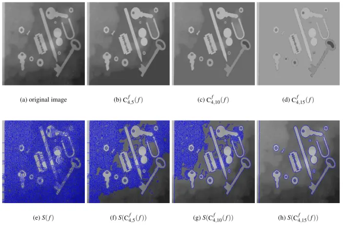
(a) original image (b) C4f,5(f) (c) C4f,10(f) (d) C4f,15(f)
(e)S(f) (f)S(C4f,5(f)) (g)S(C4f,10(f)) (h)S(C4f,15(f))
Fig. 9.Hierarchical pyramidal segmentation of the ‘Tools’ (a) image. First, the original image is decomposed using adaptive sequential closing filters (b-d). Secondly, the application of the morphological gradient followed by the watershed transformation, denoted S, achieves the images (f-h). The original image is decomposed so as to avoid an over-segmentation (e). The process S(C4f,n(f))provides a well-accepted segmentation for n≥15(g,h).
ADAPTIVE MORPHOLOGICAL HIERARCHICAL SEGMENTATION
In this last application example, the ‘tools’ test image (Fig. 9) is hierarchically segmented. The process is achieved in three steps:
1. firstly, the original image is smoothed with adaptive sequential closing filters (Eq. 35) which satisfy relevant properties (anti-size distribution and connectedness), supplying a multiscale representation,
2. secondly, the morphological gradient is computed on decomposed images,
3. finally, the watershed transform is applied to the previous images.
In this way, it leads to a hierarchical segmentation (Vachier, 2001) without any operators by reconstruction.
The resulting hierarchical segmentation supplies nested partitions of the spatial support of the
original image, which could induce a graph representation (Serra and Salembier, 1993; Vachier, 2001). Thereafter, the process C4f,noffers the expected result for n=15 or n>15. Indeed, this operator is
saturated from this value:
∀n>15 C4f,n(f) =C4f,15(f).
This characteristic has been studied and promises relevant topological properties (Debayle, 2005).
Furthermore, the resulting hierarchical segmentation, where flat zones are nested, is achieved without any operators by reconstruction (Crespoet al., 1995). Filters by reconstruction require geodesic transformations, so as to define connected operators, which are traditionally used for this kind of multiscale segmentation (Serra and Salembier, 1993; Salembier and Serra, 1995; Vachier, 2001).
IMPLEMENTATION ISSUE
The algorithms of the proposed morphological operators are built in two steps. Firstly, the AN sets are computed and stored in random access memory (RAM). The equality property (Prop. 1.3) between iso-valued points is used so as to save memory and reduce computation time. Secondly, the operators are run with the stored AN sets. In this way, AN sets are computed once time even for advanced operators, such as adaptive ASFs. Nevertheless, this methodology requires a large random access memory (RAM) so as to store all the AN sets. Moreover, the computational time of AN sets is rather long, about 2-3 minutes for of a 256×256 image, with a Pentium IV (3GHz / 2Go RAM) using the software AphelionTM and C++ language. Conversely, the running of morphological operators is faster (for example 4-5 seconds for a dilation).
CONCLUSION
The proposed spatially-variant morphological approach provides adaptive operators without any a priori knowledge of the studied image. Theoretically, such transforms possess several strong advantages such as the connectedness of the operators, contrary to the usual ones which fail to this property. In practice, it yields good results in the field of image filtering and segmentation. The idea of building spatially adaptive operators using intrinsic operational windows which locally fit to the features of an image is very promising and can suit different image processing tools, more particularly in multiscale image analysis as studied in (Debayle and Pinoli, 2005b).
Currently, the authors are interested in AN sets taking into account physical and psychophysical settings allowing to be consistent with several image formation models and with the human visual perception. In addition, other analyzing criteria are actually being studied.
ACKNOWLEDGMENT
The authors thank their colleague Yann Gavet (Ecole Nationale Sup´erieure des Mines de Saint-Etienne, France) for his computing contributions.
REFERENCES
Alvarez L, Guichard F, Lions PL, Morel JM (1993). Axioms and fundamental equations in image processing. Arch Ration Mech An 123:199–257.
Arce GR, Foster RE (1989). Detail-preserving ranked-order based filters for image processing. IEEE Trans Acoust Speech 37:83–98.
Braga Neto UdM (1996). Alternating sequential filters by adaptive-neighborhood structuring functions. In: Maragos P, Schafer RW, Butt MA, eds. Mathematical Morphology and its Applications to Image and Signal Processing. Kluwer Academic Publishers, 139-46. Buzuloiu V, Ciuc M, Rangayyan RM, Vertan C (2001).
Adaptive-neighborhood histogram equalization of color images. Electron Imaging 10:445–59.
Cech A (1966). Topological Spaces. John Wiley and Sons. Charif-Chefchaouni M, Schonfeld D (1994).
Spatially-variant mathematical morphology. In: Proceedings of the IEEE International Conference on Image Processing. Austin, Texas, USA, November 13-16, vol. 2, 555–9.
Chazallon L, Pinoli JC (1997). An automatic morphological method for aluminium grain segmentation in complex grey level images. Acta Stereol 16:119–30.
Choquet G (2000). Cours de topologie, chap. Espaces topologiques et espaces m´etriques. Paris: Dunod, 45– 51.
Ciuc M (2002). Traitement d’images multicomposantes: application `a l’imagerie couleur et radar. Ph.D. thesis, Universit´e de Savoie - Universit´e Polytechnique de Bucarest, Roumanie.
Ciuc M, Rangayyan RM, Zaharia T, Buzuloiu V (2000). Filtering noise in color images using adaptive-neighborhood statistics. Electron Imaging 9:484–94. Crespo J, Serra J, Schafer RW (1995). Theoretical aspects of
morphological filters by reconstruction. Signal Process 47:201–25.
Cuisenaire O (2005). Locally adaptable mathematical morphology. In: Proceedings of the IEEE International Conference on Image Processing. Genova, Italy, September 11-14, vol. II, 125–8.
Dakin SC, Hess RF (1997). The spatial mechanisms mediating symmetry perception. Vision Res 37:2915– 30.
Debayle J (2005). General Adaptive Neighborhood Image Processing. Ph.D. thesis, Ecole Nationale Sup´erieure des Mines, Saint-Etienne, France. In preparation. Debayle J, Pinoli JC (2005a). Adaptive-neighborhood
mathematical morphology and its applications to image filtering and segmentation. In: 9th European Congress on Stereology and Image Analysis. Zakopane, Poland; May 10-13, vol. 2, 123–30.
International Conference on Image Processing. Genova, Italy; September 11-14, vol. III, 537–40.
Gordon R, Rangayyan RM (1984). Feature enhancement of mammograms using fixed and adaptive neighborhoods. Appl Opt 23:560–4.
Heijmans HJAM, Boomgaard RVD (2000). Algebraic framework for linear and morphological scale-spaces. J Vis Commun Image R 13:269–301.
Jourlin M, Pinoli JC, Zeboudj R (1988). Contrast definition and contour detection for logarithmic images. J Microsc 156:33–40.
Laporterie F, Flouzat G, Amram O (2002). The morphological pyramid and its applications to remote sensing: Multiresolution data analysis and features extraction. Image Anal Stereol 21:49–53.
Lerallut R, Decencire E, Meyer F (2005). Image filtering using morphological amoebas. In: Ronse C, Najman L, Derenci`ere E, eds., Proceedings of the 7th International Symposium on Mathematical Morphology. Paris, France; April 18-20, 13–22. Lindeberg T (1994). Scale-space theory: a basic tool
for analysing structures at different scales. J Appl Stat 21:225–70. (Supplement on Advances in Applied Statistics: Statistics and Images: 2).
Mallat SG (1989). A theory for multiresolution decomposition: The wavelet representation. IEEE Trans Pattern Anal 11:674–93.
Matheron G (1967). El´ements pour une th´eorie des milieux poreux. Paris: Masson.
Matheron G (1988). Image Analysis and Mathematical Morphology. Volume 2: Theoretical Advances, chap. Filters and Lattices. London: Academic Press, 115–40. Paranjape RB, Rangayyan RM, Morrow WM (1994). Adaptive neighbourhood mean and median image filtering. Electron Imaging 3:360–7.
Perona P, Malik J (1990). Scale-space and edge detection using anisotropic diffusion. IEEE Trans Pattern Anal 12:629–39.
Pinoli JC (1991). A contrast definition for logarithmic images in the continuous setting. Acta Stereol 10:85– 96.
Rabie TF, Rangayyan RM, Paranjape RB (1994). Adaptive-neighborhood image deblurring. Electron Imaging 3:368–78.
Rangayyan RM, Ciuc M, Faghih F (1998). Adaptive-neighborhood filtering of images corrupted by signal-dependent noise. Appl Opt 37:4477–87.
Rangayyan RM, Das A (1998). Filtering multiplicative noise in images using adaptive region-based statistics. Electron Imaging 7:222–30.
Salembier P (1992). Structuring element adaptation for morphological filters. J Vis Commun Image R 3:115– 36.
Salembier P, Serra J (1995). Flat zones filtering, connected operators, and filters by reconstruction. IEEE Trans Image Process 4:1153–9.
Serra J (1988a). Image Analysis and Mathematical Morphology. Volume 2: Theoretical Advances, chap. Mathematical Morphology for Complete Lattices. London: Academic Press, 13–35.
Serra J (1988b). Image Analysis and Mathematical Morphology. Volume 2: Theoretical Advances, chap. Introduction to Morphological Filters. London: Academic Press, 101–14.
Serra J (1988c). Image Analysis and Mathematical Morphology. Volume 2: Theoretical Advances, chap. Alternating Sequential Filters. London: Academic Press, 203–16.
Serra J, Salembier P (1993). Connected operators and pyramids. In: Proceedings of SPIE. San Diego, USA, 65–76.
Sun FK, Maragos P (1989). Experiments on image compression using morphological pyramids. In: Proceedings of the SPIE Visual Communications and Image Processing, vol. IV, 1303–12.
Vachier C (2001). Morphological scale-space analysis and feature extraction. In: Proceedings of the IEEE International Conference on Image Processing. Thessaloniki, Greece, October, vol. 3, 676–679. Vogt RC (1994). A spatially variant, locally adaptive,
background normalization operator. In: Serra J, Soille P, eds., Mathematical Morphology and its Applications to Image Processing. Kluwer Academic Publishers, pp. 45-52.