UCLA UCLA Previously Published Works

UCLA

UCLA Previously Published Works

Centrifuge modeling studies of site response in soft clay over wide strain range Permalink

https://escholarship.org/uc/item/57b2p20n Journal

Journal of Geotechnical and Geoenvironmental Engineering, 140(2) ISSN 1090-0241 Authors Afacan, KB Brandenberg, SJ Stewart, JP Publication Date 2014-01-28 DOI 10.1061/(ASCE)GT.1943-5606.0001014 Peer reviewed

This version is the author's final version. The typeset version of the article can be found by following the URL below.

http://dx.doi.org/10.1061/(ASCE)GT.1943-5606.0001014 1

2 3

Centrifuge Modeling Studies of Site Response in Soft Clay over Wide Strain Range

by: Kamil B. Afacan1_{, Scott J. Brandenberg}2_{, M. ASCE., and Jonathan P. Stewart}3_{, F. ASCE.}

Abstract: Centrifuge models of soft clay deposits were shaken with suites of earthquake ground motions to study site response over a wide strain range. The models were constructed in an innovative hinged-plate container to effectively reproduce one dimensional ground response boundary conditions. Dense sensor arrays facilitate back-calculation of modulus reduction and damping values that show modest misfits from empirical models. Low amplitude base motions produced nearly elastic response in which ground motions were amplified through the soil column and the fundamental site period was approximately 1.0s. High intensity base motions produced shear strains higher than 10%, mobilizing shear failure in clay at stresses larger than the undrained monotonic shear strength. We attribute these high mobilized stresses to rate effects, which should be considered in strength parameter selection for nonlinear analysis. This nonlinear response de-amplified short period spectral accelerations and lengthened the site period to 3.0s. The nonlinearity in spectral amplification is parameterized in a form used for site terms in ground motion prediction equations to provide empirical constraint unavailable from ground motion databases.

1 PhD Candidate, Department of Civil and Environmental Engineering, University of California, Los Angeles, 90095-1593

2 Associate Professor and Vice Chair, Department of Civil and Environmental Engineering, University of California, Los Angeles, 90095, email: [email protected]; Corresponding Author

3Professor and Chair, Department of Civil and Environmental Engineering, University of California, Los Angeles,

4 5 6 7 8 9 10 11 12 13 14 15 16 17 18 19 20 21 3 4 5 6 7

INTRODUCTION

The influence of soil conditions on earthquake ground motions is typically evaluated in practice either through the use of simplified site amplification functions or site-specific one-dimensional (1-D) ground response analysis. Site amplification functions are typically empirically derived from ground motion data (e.g., Borcherdt, 1994), but the available data cannot fully constrain highly nonlinear site response. The nonlinear component of site amplification functions is therefore often constrained by ground response analyses for regional site profiles (e.g., Walling et al., 2008). Because site amplification functions utilize relatively generic descriptions of site condition (e.g., time-averaged shear wave velocity in the upper 30 m, Vs30), their estimates of

site amplification can be more approximate than those from ground response analysis, which use more site-specific information (e.g., Baturay and Stewart, 2003).

While both site amplification functions and site-specific analyses draw upon ground response modeling, there is considerable ambiguity on how those simulations should be performed for conditions producing large-strain site response. The two principal options for ground response analysis are equivalent linear methods, in which the soil is modeled as visco-elastic with shear modulus and damping selected to be compatible with the level of mobilized shear strain, or nonlinear methods, in which plasticity models are utilized to simulate the soil's constitutive behavior. The equivalent linear method has historically been more popular than nonlinear analysis in practice (Kramer and Paulsen 2004), although there is a general consensus that nonlinear analysis is preferred for high intensity motions that mobilize large-strain response in the soil (i.e., for shear strains approaching 1% or more), and nonlinear methods are now 22 23 24 25 26 27 28 29 30 31 32 33 34 35 36 37 38 39 40 41 42 43

more commonly used in practice. A number of hurdles related to parameter selection and other matters have tempered the use of nonlinear methods, although many of those issues have been addressed in recent work (e.g., Kwok et al., 2007; Stewart and Kwok, 2008; Phillips and Hashash, 2009; and Hashash et al., 2010).

The work described in this manuscript was undertaken to fill the gap in available data for 1-D soil response at very large strains approaching shear failure for the purpose of ultimately validating nonlinear ground response analysis methods, and for validating the nonlinear component of relatively simplified amplification functions. This problem is of considerable practical importance because design-level ground motions in seismically active regions are strong, and in soft soils will induce large strain response of the type investigated here. Moreover, large-strain response is the condition where nonlinear analysis is thought to be most useful, yet for which the available data for validation is most sparse (e.g., Yee et al., 2013).

We describe a ground response data set from centrifuge experiments in which small-and large-strain responses are recorded. We sought boundary conditions compatible with 1-D vertical shear wave propagation, which was not achieved in previous large centrifuge site response models (e.g., Wilson et al. 1997), though it was achieved using small centrifuge models with relatively sparse sensor arrays (e.g., Fiegel 1995). In this study, two centrifuge models were constructed and tested on the 9m radius geotechnical centrifuge at the NEES@UCDavis experimental facility. The models were composed of soft young bay mud, which is naturally occurring clay whose dynamic properties are well characterized in the literature. We describe the centrifuge models (soil properties, container), the ground motions applied in the testing, and the principal test results (stress-strain curves, modulus reduction and damping, and 44 45 46 47 48 49 50 51 52 53 54 55 56 57 58 59 60 61 62 63 64 65

site amplification). Due to length restrictions, we defer nonlinear ground response analysis of the experiment to a later publication.

CENTRIFUGE MODELS

Specimen Configuration and Construction

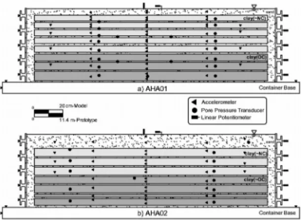
As shown in Fig. 1, two centrifuge models called AHA01 and AHA02 were constructed in a hinged plate container from layers of soft San Francisco bay mud. The profiles consisted of a layer of sand over lightly overconsolidated (OCR = 1 to 1.2) bay mud atop overconsolidated bay mud (OCR = 2 to 4). This profile is consistent with natural geologic conditions in many parts of the San Francisco bay area (e.g., Merritt Sand over young bay mud in many parts of Oakland). San Francisco bay mud was selected for this study because it is naturally occurring clay from a seismically active region, its dynamic properties have been previously studied, and ground motion recordings are available for multiple sites that are underlain by bay mud from which prior work has evaluated site amplification that can be compared to the results of this study. The high plasticity of bay mud renders low permeability and slow consolidation times, so thin layers of dense Monterey sand were placed between the clay layers to act as drainage boundaries to facilitate specimen construction. These thin sand layers likely introduced a small amount of phase shift as the waves propagated vertically through the soil profile, but are not anticipated to significantly alter site response considering that they are stiff, strong, and thin relative to the clay layers, and also thin relative to the wavelengths of the vertically propagating shear waves (e.g., Santamarina et al. 2001).

66 67 68 69 70 71 72 73 74 75 76 77 78 79 80 81 82 83 84 85 86

Figure 1. Elevation view of centrifuge models AHA01 and AHA02

Models were constructed by mixing the bay mud as slurry at a water content of 1.4 times its liquid limit, pouring enough slurry into the model container to obtain the proper lift thickness after consolidation, placing pore pressure transducers (PPTs) in the center of the slurry, and consolidating with a hydraulic press. Consolidation from slurry was performed before the model container was placed on the centrifuge arm. Additional details on specimen construction and instrumentation are presented by Harounian et al. (2010) and Afacan et al. (2011). PPTs were used to monitor excess pore pressure and consolidation was deemed complete when the degree of consolidation at the center of the clay lift had reached at least 95%. Accelerometers and bender elements were installed within completed lifts by cutting small holes in the clay, placing the instruments, and hand-backfilling around the instruments with cuttings. Linear potentiometers measured settlement and lateral displacement. A total of 106 accelerometers, 34 pore pressure transducers (PPTs), and 22 linear potentiometers were utilized. 87 88 89 90 91 92 93 94 95 96 97 98 99 100 101 102

Properties of Bay Mud Materials

Table 1 shows the principal index properties of the bay mud and sand materials used in specimen construction. The bay mud has a PI of 43 and USCS classification of MH. The sand material has no fines and a USCS classification of SP. In this section, we focus principally on the shear-wave velocity of both materials and the monotonic undrained shear strength of the clay materials. These are the most directly relevant soil properties for ground response analysis. Table 1. Bay mud and sand soil properties.

Parameter Bay Mud Sand USCS Classification MH SP Specific Gravity 2.65 2.64 Unit Weight,  (kN/m3₎a _{16 to 17 19.8} Compression index, Cc 0.43 --Recompression index, Cr 0.04 --PL (%) 40-43 --LL (%) 84-86 --FC (%) 100 0 Friction Angle, φ’(°)b ₂₀ -a

(

)

We originally sought to develop a profile of shear wave velocity in the centrifuge specimen using bender element tests. One source and two receiver bender elements were placed in each clay layer following consolidation, and travel times were measured using cross-correlation of the receiver signals. Receiver-to-receiver measurements cancel sources of peripheral phase lag such as trigger delay, rise time in the piezo crystals, and soil-bender interaction that are present in source-to-receiver measurements (e.g., Lee and Santamarina, 2005; Brandenberg et al. 2008). Unfortunately, the insulator coating on many of the bender 103 104 105 106 107 108 109 110 111 112 113 114 115 116 117 118 119

elements was inadequate, and electrical current leaked from the source element into the soil and the direct arrival of this current at the receiver obscured the reading of physical waves in the receiver signals. As a result of these difficulties, physically meaningful bender element measurements were recovered for only a single clay lift in AHA02 and for the upper sand layer.

Because the bender elements only provided a measurement of Vs in one lift of clay

rather than all of the lifts as originally intended, we utilized the available measurement to calibrate relations from the literature between the maximum (small strain) shear modulus, Gmax,

confining pressure, and OCR. Yamada et al. (2008) provide the following general expression for the effective stress-dependence of Gmax in normally consolidated soil (the equation is slightly

modified here to become dimensionless):

n a mc a p p G          ' max _  (1)

Where n=1.0 for clay, mc’ is the mean effectives stress, and  is dependent on soil type. Based

on a similar relation by Hardin and Drnevich (1972), we expect Gmax to be proportional to OCRc

(where c = 0.3 for clay with PI=40). We insert this term into Eq (1) and re-write the expression in terms of vertical effective consolidation stress vc’, as follows:

n a vc c n a p OCR K p G                 ' 0 max 3 2 1   (2)

where K0 is the coefficient of lateral earth pressure at rest. The available bender element data is

from a clay layer for which vc' = 117 kPa, sat=16.4 kN/m3_{, and OCR=1.15; V}

s=108m/s was 120 121 122 123 124 125 126 127 128 129 130 131 132 133 134 135 136 137

measured in this layer. Converting Vs to Gmax using the classical relation  max G V_s  (where 

is mass density) and applying K0 = (1-sin) OCR sin = 0.69 [Jaky (1944) and Schmidt (1966)], we

compute =202, which is consistent with prior experience for similar materials (Yamada et al., 2008). Values of Gmax are then obtained for other layers using = 202 in Eq. (2), with the results

shown in Fig. 2 following conversion to Vs. 138

139 140 141 142

Figure 2. Profiles of vertical effective stress, shear wave velocity, and undrained shear strength. The in-flight su profile was computed using Eq. 3, while vane shear tests were performed after

spin-down. 143 144 145 146 147

We apply a similar approach for seismic velocities in sand. In this case, the overburden scaling coefficient is n=0.5 (Yamada et al., 2008) and the OCR scaling coefficient is c=0 (Hardin and Drnevich, 1972). A shear wave velocity measurement indicating Vs = 138 m/s was obtained

from bender element data in the upper sand layer in AHA02 for which vc’=28kPa. Using unit weight of 19.8kN/m3_{, we compute =821 for the sand materials. Values of G}

max and Vs for all

sand layers are then computed using Eq. (2) with the results shown in Fig. 2. Using the profiles in Fig. 2, the values of Vs30 and site period are 114m/s and 1.1 s for AHA01 and 126m/s and 0.95s

for AHA02.

The profiles in Fig. 2 were tested by comparing their implied theoretical travel times from the base of the model container to each sensor position to those measured when the base of the model container was shaken with a high frequency (500 Hz model scale) low amplitude harmonic motion. The high frequency motion was selected to improve resolution in travel time measurements. Reasonable agreement was observed in a least-squares sense (details in Afacan et al. 2011), and the measured travel time values were within 10% of those predicted by Eq. 2.

The shear strength of the clay was measured using a small hand vane device following spin-down of the centrifuge, with the results in Fig. 2. The measured shear strengths are potentially biased relative to those in effect under “in flight” conditions as a result of reduced effective stresses due to swelling of the clay during the gradual spin-down of the centrifuge which requires about 20 minutes. Changes in pore pressure due to swelling were observed in PPT readings in the overconsolidated clay layers. The in-flight shear strengths in Fig. 2 were derived from strength normalization concepts (Ladd, 1991):

148 149 150 151 152 153 154 155 156 157 158 159 160 161 162 163 164 165 166 167 168

8 . 0 ' 0.22 OCR S vc u _{ }  (3)

where 0.22 is the undrained strength ratio of the same bay mud material measured in direct simple shear tests by Park (2011), and 0.8 = 0.88(1-Cr/Cc) is the recommended exponent from

Ladd (1991) for homogenous sedimentary clays of low to moderate sensitivity. As shown in Fig. 2, this relation produces good agreement with measured vane shear strengths in low-OCR layers relatively unaffected by swelling during spin-down. Vane shear strengths in the deeper more heavily overconsolidated layers were lower than predicted in Eq. (3), which is likely due to a decrease in effective stress due to more rapid consolidation of these stiff layers during spin-down.

Model Container

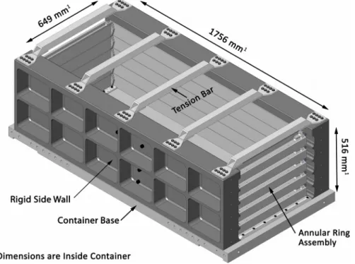
The present test sequence was the first to utilize the NEES@UCDavis hinged-plate model container (HPC) illustrated in Fig. 3. The HPC consists of five steel annular rings with end plates that are free to rotate (details can be found on the NEES@UCDavis website nees.ucdavis.edu). Each ring rests atop ball bearings supported by rigid side walls, and the container exhibits essentially zero shear stiffness (an empty container can easily be deformed by hand). Accordingly, the model stiffness is controlled by the soil inside the container with essentially zero contribution from the container itself. For this reason, the container is better suited to site response studies than comparatively stiff shear beam container systems used in prior testing on the UC Davis large centrifuge. The principal limitation of the container relative to “ideal” boundary conditions for site response is that it has finite mass that will contribute to the 169 170 171 172 173 174 175 176 177 178 179 180 181 182 183 184 185 186 187 188

dynamic response of the soil model. The mass of each ring assembly is 25 kg (125 kg total for all five rings), which is approximately 12% of the mass of the contained soil.

Figure 3. NEES@UCDavis hinged-plate container used in this study (Lars Pedersen, personal communication).

GROUND MOTIONS

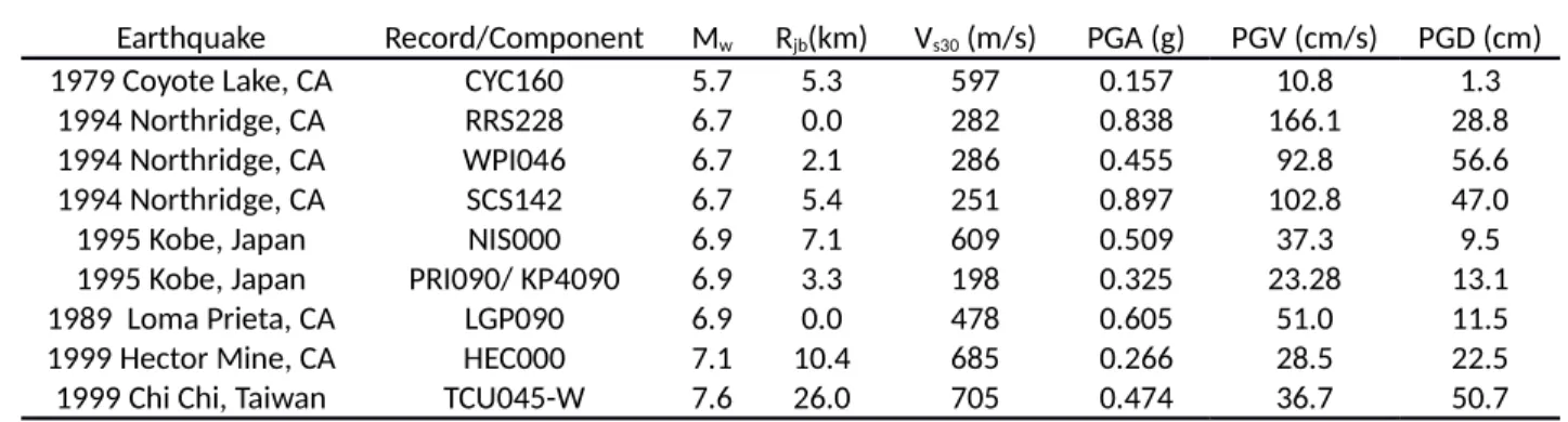
The base of the model container was shaken by a sequence of ground motions that included (i) scaled versions of earthquake recordings, (ii) small amplitude sine sweeps for the purpose of identifying the small-strain properties of the soil model, and (iii) small amplitude sine waves having approximately 20 cycles. We focus herein on the data produced by the scaled earthquake motions; results for other motions are given in data reports (Harounian et al. 2010a; Afacan et al. 2011). The selected ground motions are listed in Table 2, and response spectra are plotted in Fig. 4. The digital ground motion records and the metadata were obtained from the 189 190 191 192 193 194 195 196 197 198 199 200 201 202

PEER-NGA ground motion database (Chiou et al, 2008), and subsequently conditioned for use on the centrifuge. The selected motions cover a range of site conditions likely to exist beneath soft clay deposits (Vs30 = 198 to 705 m/s), and to cover a range of magnitudes that contribute

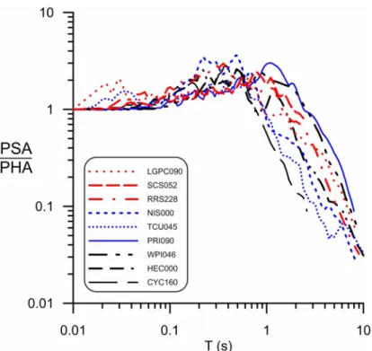
significantly to seismic hazard in many seismically active crustal regions. Furthermore, the peaks in the response spectra range from approximately 0.3s to 2s, which straddles the site period. In some cases, multiple scaled versions of the same ground motion were imposed on the model to observe effects of amplitude for the same motion, while in other cases a large amplitude motion was only applied once to mobilize large shear strains in the model. Excess pore pressures mobilized in the clay layers during shaking were small, and sufficient time was permitted between each sequential shake to permit these small excess pore pressures to dissipate.

Table 2. Characteristics of recorded earthquake ground motions utilized in this study. Motion and record/component codes are from PEER-NGA database (Chiou et al., 2008)

Earthquake Record/Component Mw Rjb(km) Vs30 (m/s) PGA (g) PGV (cm/s) PGD (cm)

1979 Coyote Lake, CA CYC160 5.7 5.3 597 0.157 10.8 1.3 1994 Northridge, CA RRS228 6.7 0.0 282 0.838 166.1 28.8 1994 Northridge, CA WPI046 6.7 2.1 286 0.455 92.8 56.6 1994 Northridge, CA SCS142 6.7 5.4 251 0.897 102.8 47.0 1995 Kobe, Japan NIS000 6.9 7.1 609 0.509 37.3 9.5 1995 Kobe, Japan PRI090/ KP4090 6.9 3.3 198 0.325 23.28 13.1 1989 Loma Prieta, CA LGP090 6.9 0.0 478 0.605 51.0 11.5 1999 Hector Mine, CA HEC000 7.1 10.4 685 0.266 28.5 22.5 1999 Chi Chi, Taiwan TCU045-W 7.6 26.0 705 0.474 36.7 50.7 203 204 205 206 207 208 209 210 211 212 213 214 215 216 217 218

Figure 4. Response spectra of the ground motions utilized in this study.

Fig. 5 shows the peak horizontal acceleration recorded in the soil near the base of the centrifuge models (PHAb) and recorded near the ground surface (PHA0). We generally see

amplification for PHAb ≤ 0.2g and de-amplification for PHAb ≥ 0.3g, with mixed results at

intermediate amplitudes. These varying levels of site amplification indicate nonlinearity. 219 220 221 222 223 224 225 226

Figure 5. Peak base acceleration (PHAb) and surface acceleration (PHA0) recorded in the

centrifuge models for tests involving earthquake ground motion excitation.

The centrifuge shaking table is able to replicate key features of the earthquake motions, although some differences arise from imperfections in the feedback control loop, particularly at high frequencies. Therefore, the recorded base motions should always be used in lieu of the command motions when analyzing the model response. Some of the motions utilized herein were conditioned for use on the centrifuge prior to the present work by Mason et al. (2010). Furthermore, the motions on the base plate of the model container are different from the motions within the soil near the base of the model container. This is likely caused by slip between the latex membrane and container base. For this reason, we herein interpret the most deeply embedded ground motion recording as being representative of the base motion.

TEST DATA

All experimental data are uploaded to the NEEShub central data repository (Harounian et al. 2013a,b), and details of the data processing methods utilized to convert the raw recorded data files into prototype engineering units are included in the data reports. In addition to recorded data, several derived quantities (e.g., 5% damped pseudo-acceleration response spectra) are archived in NEEShub. The data are presented in prototype units, and were converted using scale factors defined in the data reports (Harounian et al. 2010, Afacan et al. 2011). Acceleration time series were high-pass filtered in the frequency domain using an acausal Butterworth filter to 227 228 229 230 231 232 233 234 235 236 237 238 239 240 241 242 243 244 245 246 247

described by Boore and Bommer (2005), which is intended to apply the smallest possible amount of filtering while achieving realistic velocity and displacement.

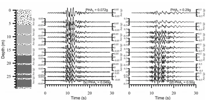
An example of corrected acceleration histories from the dense instrument array in the center of model AHA02 for the LGPC090 motion with PHAb = 0.049g and 0.50g are presented in

Fig. 6. At the ground surface, the small amplitude base motion was amplified by 1.5 (PGA0 =

0.072 g) whereas the large amplitude motion was de-amplified at high frequencies by 0.58 (PGA0 = 0.29 g). A change in frequency content is also evident for the strong base motion due to

nonlinear site response.

Figure 6. Acceleration time series for motion LGPC090 for (a) PHAb=0.049g and (b) PHAb=0.50g.

PERFORMANCE OF HINGED-PLATE CONTAINER

A number of previous centrifuge modeling studies utilized flexible shear beam (FSB) containers consisting of aluminum or steel rings separated by rubber layers that allow the container to deform in a step-wise manner. Container shear stiffness introduces an undesired boundary 249 250 251 252 253 254 255 256 257 258 259 260 261 262 263

condition for 1-D site response modeling due to reflections of seismic energy from the container walls. These undesired boundary conditions cause horizontal spatial variation in the ground motions, with the largest effects near the container rings and smaller effects near the center of the soil model. The effects are anticipated to be largest for soft soil conditions, and may be negligible for stiff soil profiles for which the finite container stiffness is a smaller fraction of the system stiffness. Similarly, the effects are anticipated to increase with shaking intensity due to reduction in the shear modulus of the soil at large shear strains.

Undesirable performance of shear beam containers is likely to have affected measured responses in previous studies. For example, Lai et al. (2001) and Elgamal et al. (2005) presented a test program on dense sand constructed in an FSB container. They found that damping values back-calculated from acceleration array data were higher than empirical curves. Utilizing wavelet analysis to analyze the time-dependent frequency content of vertical array acceleration data, they observed that near the walls of the container the frequency content of the ground motion was spread over a larger band than the motions near the center of the model. Moreover, shear strains were larger near the walls of the shear beam container for saturated sand models. These observations were attributed in part to p-waves generated at the container boundary. They acknowledged that container performance might contribute to the high damping values, but indicated that further investigation was needed to explain the experimental finding. Fiegel (1995) implemented a hinged-plate container on the small 1m diameter Schaevitz centrifuge at UC Davis, and found that the ground motions near the center of the container were very similar to those offset from the centerline at the same elevation. 264 265 266 267 268 269 270 271 272 273 274 275 276 277 278 279 280 281 282 283 284

Furthermore, significantly more ground motion amplification was observed in a rigid container compared with the hinged-plate container for high intensity input motions.

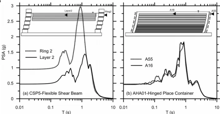
We examine the influence of container stiffness by comparing data from test CSP5 (Wilson et al. 1997) with test AHA01. This comparison was chosen because (i) CSP5 utilized a FSB container whereas AHA01 utilized the HPC container, (ii) both models contained layers of lightly overconsolidated San Francisco Bay mud, and (iii) the same ground motion recorded at Port Island during the 1995 Kobe earthquake was input to the base of both models. Furthermore, a high intensity ground motion is selected because large strains were induced in the clay thereby reducing its shear stiffness, exacerbating any undesired container effects. Acceleration response spectra (5% damping) for a ground motion recorded from an accelerometer embedded near the surface of the soft clay deposit, and on the container ring at the same elevation are shown in Fig. 7. The ground motion in the clay layer should be identical to the motion on the container at the same elevation if 1-D site response conditions were achieved during the tests. The two response spectra for CSP5 exhibit significant differences at short periods, with the container ground motion approximately twice as large as the soil ground motion. On the other hand, the two response spectra for AHA01 are essentially identical at all periods. This indicates that the HPC container produced better 1-D boundary conditions than the FSB container, and is therefore better suited for site response modeling.

285 286 287 288 289 290 291 292 293 294 295 296 297 298 299 300 301 302 303

Figure 7. Acceleration response spectra (5% damping) near the top of a soft clay layer and on the container ring at the same elevation for (a) test CSP5 tested in a flexible shear beam container (Wilson et al., 1997), and (b) test AHA01 tested in a hinged-plate container. Deformations exaggerated, and pile foundations from CSP5 omitted for clarity.

304 305 306 307 308 309 310

DATA INTERPRETATION

Derivation of Shear Stresses and Strains

The time-dependence of shear stresses and shear strains was evaluated at selected depths within clay layers from the corrected data using the procedure of Zeghal and Elgamal (1994). Referring to Fig. 8, shear stress at depth z and time t was computed by summing the inertia of overlying soil as:

 

_

 

where index i denotes discrete depth intervals above depth z, each of which has an accelerometer at the middle of the depth interval (i.e., depth z occurs at the boundary between intervals i and i+1); N(z) is the number of such depth intervals; i is mass density for depth

interval i;

 

is the horizontal acceleration for depth interval i at time t (from the corrected

acceleration time series), and zi is the tributary depth associated with interval i. 311 312 313 314 315 316 317 318 319 320 321 322 323

Figure 8. Schematic illustration of profile layering used for stress and strain computations.

The average shear strain at depth z was computed assuming 1-D wave propagation conditions (i.e.,  = ∂u/∂z) as:

 





The numerator in Eq. 5 represents the differential horizontal displacement between the accelerometers immediately above and below depth z, and the denominator represents the vertical distance between those accelerometers.

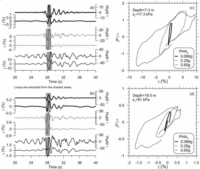
An example set of stress histories, strain histories, and normalized stress-strain curves at two depths are shown in Fig. 9. Shear stresses are normalized by the undrained monotonic shear strength computed using Eq. (3). The stress and strain histories are shown for the RRS228 motion with various base motion intensities (PHAb = 0.069g, 0.29g and 0.60g). The normalized

stress-strain curves span approximately one loading cycle at the time interval in the strain history when the peak strain occurs.

324 325 326 327 328 329 330 331 332 333 334 335 336 337

Figure 9. Stress and strain histories evaluated in relatively soft and firm clay layers when subjected to motion RRS228 at (a) 7.3 m depth, (b) 18.5 m depth and corresponding stress-strain loops extracted from the shaded areas (c) at 7.3 m depth and (d) 18.5 m depth.

The lowest-amplitude stress and strain histories (for PHAb = 0.069g in Fig. 9 a,b) have

similar waveforms, which is generally compatible with the assumption of linear (or equivalent-linear) analyses in which the strain history scaled by a constant shear modulus produces the stress history (along with some phase shift from damping). This similarity of waveforms breaks down at larger strains (e.g., PHAb = 0.60g in Fig. 9a), where the stress/strain ratio is higher for 338 339 340 341 342 343 344 345 346 347

the small cycles between 20 and 27s than for the large cycle at 28s. The different stress/strain ratios with time for the large intensity motion is caused by the significant reduction in shear modulus associated with such large shear strains. Equivalent linear analysis, in which the shear modulus is independent of time, cannot capture this type of behavior.

Turning next to the stress-strain loops, secant shear modulus decreases as cyclic strain increases in a manner that is similar to traditional cyclic laboratory tests. However, the stress-strain loops are not smooth due to the broadband nature of the input motions. At a depth of 7.3m near the center of the uppermost lift of clay, the shear strain for the motion with PHAb =

0.60g exceeds 10%, while the shear stress exceeds the monotonic undrained shear strength by more than 50%. Strain rate effects explain why the mobilized shear stress exceeded the monotonic undrained strength, as demonstrated later. At a depth of 18.5m, where the clay was overconsolidated, the shear strains are lower (near 1%), and mobilized shear stresses do not reach the monotonic undrained strength.

Modulus Reduction and Damping Behavior

Published modulus reduction and damping curves are generally empirically verified to shear strains up to approximately 0.3 to 0.5%, and are often fit with hyperbolic functions that provide a good match with data in this range of strains (e.g., Darendeli, 2001). In practice, these functional forms are often extrapolated to higher shear strains beyond the calibration range, and can provide implied shear strengths that are significantly different from the soil shear strength (e.g., Stewart and Kwok 2008). It is of interest to compare the modulus reduction and damping behavior evaluated from the centrifuge test data against these published curves, 348 349 350 351 352 353 354 355 356 357 358 359 360 361 362 363 364 365 366 367 368

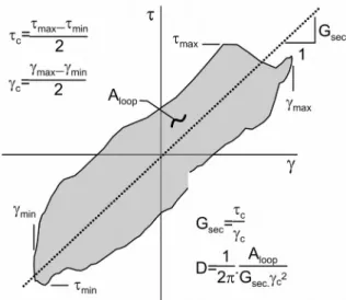
Referring to the schematic stress-strain loop in Fig. 10, we apply the approach of Zeghal and Elgamal (1994) to compute secant shear modulus, Gsec, and damping, D. Stress-strain loops

like those shown in Fig. 9 were generated for each ground motion imposed on the models, and

Gsec and D were computed. The area of each loop required to obtain D was computed using

trapezoidal integration. The small strain shear modulus was computed as Gmax = Vs2, and

normalized shear modulus Gsec/Gmax and D were plotted versus shear strain in Fig.10a-b.

Extracting Gsec and D from the centrifuge data is more complicated than with strain-controlled

harmonic laboratory tests because the broadband excitation in the centrifuge models caused asymmetric stress-strain loops that sometimes did not close (e.g., Fig. 10). Furthermore, shear strains smaller than about 0.02% could not be accurately measured in the centrifuge because the signal to noise ratio in the acceleration records is too low at small shaking levels, and because of A/D conversion resolution. Therefore, the data in Fig. 11 are plotted only for c >

0.02%.

Figure 10. Schematic illustration of non-symmetric stress strain loop and quantities used for evaluation of secant modulus Gsec and hysteretic damping D

370 371 372 373 374 375 376 377 378 379 380 381 382 383 384 385

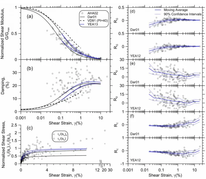
Figure 11. (a) Normalized shear modulus curves, (b) damping curves and (c) normalized shear stress vs shear strain curves for AHA02 and (d) modulus reduction residuals, (e) damping residuals, (f) stress residuals for Dar01 and YEA13 models. In legend, Dar01 = Darendeli (2001), VD91 = Vucetic and Dobry (1991), and YEA13 = Yee et al. (2013). Parameter (su)d is the strain

rate compatible shear strength.

Also shown in Fig.10a are the recommended modulus reduction relations from Vucetic and Dobry (1991) and Darendeli (2001). Two curves are plotted for the Darendeli relation to bound 386 387 388 389 390 391 392 393 394 395 396

the range of consolidation stress and overconsolidation ratio for the clay in the centrifuge models (the Vucetic and Dobry relation is independent of confining pressure).The Darendeli model is extended to 10% (beyond the upper bound of experimental validation) for the purpose of comparing with the centrifuge test data. In general, Darendeli’s functional form appears to provide a reasonable characterization of the observed modulus reduction behavior in the centrifuge models, although a more formal assessment of bias is given below.

Damping values computed from the centrifuge test data (Fig. 11b) exhibit significant scatter, and tend to be higher than the published trends. This observation is similar to several studies that have utilized 1-D array data to characterize stress-strain behavior for centrifuge models and field arrays (e.g., Elgamal et al. 2001, Tsai and Hashash 2009).

Fig. 11c shows backbone stress-strain data in which shear stress is normalized by the undrained monotonic shear strength (su) and a higher, strain rate-compatible shear strength,

(su)d. According to Sheahan et al. (1996), undrained shear strength increases approximately 9%

per log cycle increase of strain rate,

. The monotonic undrained strength was measured in the

laboratory at a traditional

 (e.g., 0.006%/s to reach 10% strain in 30 minutes), whereas as high as 6000%/s (model scale) was observed during the centrifuge tests. This six order of

magnitude increase in

 corresponds to

_{( )}

s s = = Values of (su)d were obtained for each motion by computing the peak strain rate mobilized during each motion, and 397 398 399 400 401 402 403 404 405 406 407 408 409 410 411 412 413 414

correcting as demonstrated above. This is admittedly an extrapolation of Sheahan’s findings because strain rates mobilized in the centrifuge were much higher than those imposed in laboratory studies. In Fig 10c, the c/(su)d values approach unity at high strain values, whereas

c/su values significantly exceed unity. This shows that strain-rate corrections should be applied

to shear strengths for site response problems. Strain rates mobilized in centrifuge models are approximately two orders of magnitude larger than those anticipated for prototype conditions, but the increase in shear strength is nevertheless significant. We recognize that rate effects may also be present for shear stiffness (i.e., Vs or Gmax), but in this case the geophysical

measurements were made at strain rates that were not significantly different from those mobilized during shaking since we used bender element measurements and high frequency harmonic motions to measure the Vs profile. Therefore we did not correct shear stiffness for

rate effects.

Along with the data, Fig. 11c also shows stress-strain curves implied by Darendeli’s functional form. The shear strength implied by extrapolating the function to high strain is significantly smaller than the monotonic undrained strength of the clay, which is clear from the stress-strain curves (Fig. 11c) but not evident from the modulus reduction plots (Fig. 11a). Yee et al. (2013) proposed a procedure to adjust the modulus reduction curve to provide the desired undrained shear strength [taken as (su)d] at high strains. The resulting modulus reduction,

damping, and stress-strain curves are shown with dotted lines in Figs. 11a-c. The modified stress-strain relation asymptotically approaches (su)d as shear strain goes to infinity, which

provides a better match to the c/(su)d data. The improved fit is not visible from the modulus

reduction curves, which are poorly suited to visualization of large-strain behavior (i.e., very 415 416 417 418 419 420 421 422 423 424 425 426 427 428 429 430 431 432 433 434 435 436

small variations in modulus reduction at high strain cause large variations in implied shear stress).

The data points in Figs. 11a-c correspond to a variety of v' and OCR values, complicating

the data-model comparison. To facilitate a more formal evaluation of model performance, we compute residuals defined as the difference between the recorded data and the models (Sheather, 2009) for modulus reduction (RG), damping (RD), and normalized stress (R) as follows:

sec sec max max G data Model G G R G G æ ö æ ö =_{ç ÷} - _{ç ÷} è ø è ø (6a) D data Model R =D - D (6b)

 

Model equations are omitted for brevity (they can be found in the references), but include effects of consolidation stress, OCR, and plasticity index. Within the strain range of range of applicability of the Darendeli model (c ≤  0.3%), modulus reduction residuals (Fig. 11d)

generally indicate negative bias (i.e., model too linear) whereas damping residuals indicate positive residuals (model damping too low). The dispersion of modulus reduction and damping results can be represented by standard deviations of the residuals in Figs. 10d-e, which are 0.083 and 8.33%, respectively, for  = 0.3%. These can be compared to standard deviations of 0.065 and 2.04% over a comparable strain range for the data used to develop the Darendeli model. 437 438 439 440 441 442 443 444 445 446 447 448 449 450 451 452 453 454

At large strains, the most relevant results are the stress residuals (Fig. 11f), which are significantly positive for Darendeli (model underpredicts stress) and close to zero for Yee et al. These differences in large strain soil properties have been shown to significantly affect the results of nonlinear ground response analyses, as shown for example in comparisons to vertical array data by Yee et al. (2013).

Spectral Amplification of Ground Motions

Having described dynamic properties of the clay during the centrifuge tests, we now turn our attention to spectral amplification. The term ‘spectral amplification’ refers to the ratio of the 5% damped pseudo acceleration (PSA) response spectra of the recorded ground surface and container base motions:

 

 

 

Response spectra for the LGPC090 motion at three intensity levels are shown in Fig. 12a, while Fig. 12b shows the period-dependent spectral amplification values, F. Several trends are evident from the spectra and amplification plots. First, amplification levels are relatively flat for

T< 0.5s and are strongly variable with the level of input motion (weak motions producing amplification near 2 and strong motions producing amplification near 0.5). Second, relatively narrow-band and substantial amplification up to a factor of 3 occurs near the elastic site period (near 1.0s) for the weakest motion, whereas stronger motions both lengthen the period to as much as 3s and broaden the spectral peak. These effects are expected because of the modulus decrease and damping increase when the soil is subjected to increased shaking intensities. 455 456 457 458 459 460 461 462 463 464 465 466 467 468 469 470 471 472 473 474

Third, for periods beyond the site period, amplification levels are larger than 1.0, with the relative levels of amplification being the inverse of the short period trends (amplification increasing with strength of input motion). This apparent reversal of traditionally understood nonlinear effects appears to result from the transfer of energy to increasingly long periods as the soil softens. The response spectra extend to periods of only 5s because low frequency noise in the acceleration records rendered poor signal-to-noise ratio at longer periods.

Figure 12. (a) Acceleration response spectra for base and top of the model for the LGPC090 ground motion for different PHAb=0.049g, 0.18g, 0.50 g respectively and (b) Amplification

Factors for the LGPC090 ground motion.

Spectral amplification is parameterized as a function of Vs30 in the site terms used in the

Next Generation Attenuation (NGA) ground motion prediction equations (GMPEs). GMPE site terms represent the ratio of mean ground motion for a given V to that for a reference velocity 475 476 477 478 479 480 481 482 483 484 485 486 487 488

(Vref), with both motions corresponding to outcropping (ground surface) conditions. The

functional form of the site terms includes a linear amplification term that captures the scaling of ground motion with Vs30 and a nonlinear term that captures the variation of F with PHAb (or a

reference PSA term) for the given Vs30. The centrifuge models have a strong impedance contrast

at the base of the clay (the container base is essentially rigid), which is atypical of field conditions. Moreover, spectral amplification from Eq. (7) is defined as surface-to-base rather than surface-to-surface for two different site conditions. Accordingly, we do not expect a perfect match to the overall level of site amplification (represented by the linear component of site terms) but we consider the test data to be useful for checking the nonlinear terms in the GMPEs.

To investigate the nonlinearity implied by the test results, we plot in Fig. 13 spectral amplification factors (F) for T = 0.01s, 0.1s, 1.0s, and 3.0s versus PHAb. Also shown for

comparison are the predictions of the site term in the Boore and Atkinson (2008) GMPE, which is adapted from the model of Choi and Stewart (2005). There are several interesting features in these plots. First, the slopes of the ln(F) vs. ln(PHAb) relations for large PHAb, which are denoted

as b values and effectively parameterize the nonlinearity, are similar between the GMPE and data. This is not necessarily expected, because the GMPE site term was derived for sites generally significantly stiffer than those in the centrifuge tests (even the NEHRP Class E sites used in the model development), so the comparison here represents an extrapolation of the model. Second, we do not see clear evidence of an inflection point in the ln(F) vs. ln(PHAb) data

for very strong PHAb, where soil failure is occurring. This suggest that amplification models with

a simple linear representation of the ln(F) - ln(PHA ) relationship at large PHA may be 489 490 491 492 493 494 495 496 497 498 499 500 501 502 503 504 505 506 507 508 509 510

acceptable. Third, the data for T = 0.1s and 1.0s indicate a clear break from relatively linear site response (roughly independent of PHAb) for low input motion levels to nonlinear at transitional

PHAb values ranging from about 0.01g to 0.1g. Roughly similar transitional PHAb values are

reflected in the GMPE site terms, as shown in Fig. 13. Fourth, the data for T = 3.0s indicate a generally flat trend with PHAb, potentially even trending upward (positive b) for high values of

PHAb. This effect is not captured by the model, which retains a reduced level of nonlinearity at

long period.

Figure 13. Amplification factor versus peak horizontal acceleration at (a) T=0.01 s, (b) T=0.1 s, (c) T=1 s and (d) T=3 s for all of the ground motions recorded in this study. In legend, BA08 = Boore 511 512 513 514 515 516 517 518 519 520 521

In Fig. 14 we plot the period-dependence of slope parameter b computed from the test data using results with PHAb ≥ 0.1g. Also shown in Fig. 14 are the trends of slope identified in

previous models derived from ground motion data (Choi and Stewart 2005) and equivalent-linear simulations (Walling et al. 2008). The principal difference between b value trends in the two prior models is the significant dip between 0.1s and 1.0s in the simulation-based results (Walling et al. 2008). Interestingly, the centrifuge data are more consistent with the relatively flat trend of the model derived from data (Choi and Stewart 2005).

Figure 14. Slope of the amplification factors from centrifuge test data compared with similar slopes from data- and simulation-driven models. In legend, CS05 = Choi and Stewart (2005), BA08 = Boore and Atkinson (2008), and WEA08 = Walling et al (2008).

523 524 525 526 527 528 529 530 531 532 533 534 535

CONCLUSIONS

We present a centrifuge modeling study of site response in soft clay spanning a broad strain range that includes nearly linear and strongly nonlinear soil behavior. The model response was characterized using dense sensor arrays and 1-D shaking conditions were achieved using an innovative hinged-plate container. The test data provides a useful resource for validating nonlinear site response from empirical models and wave propagation routines.

Modulus reduction and damping values back-calculated from the recorded acceleration data indicate modest misfit relative to empirical models within the strain range of applicability of those models (c< 0.3%). The bias is towards the models having too-high modulus

reduction at low strain and too-low damping. The damping values exhibited significant scatter as a result of the complex shapes of the hysteresis loops that result from broadband excitation. Perhaps the most significant aspect of the observed soil behavior was a large-strain response in which mobilized shear stresses significantly exceeded the undrained monotonic shear strength by factors on the order of 1.5 to 2.0. These large stresses mobilize at shear strains beyond approximately 5%. We attribute these high stresses to strain-rate effects that temporarily increase the available shear resistance in the clay during strong shaking. Following the recommendation of Sheahan et al. (1996) that shear strength increases by 9% per log-cycle increase in strain rate, shear strength at the model scale strain rates observed in the centrifuge models would be 67% higher than observed at typical laboratory strain rates. Although strain rates in the centrifuge are unrealistically high, strength increases on the order 40% would be expected based on the prototype strain rates more representative of field conditions compared with the much lower strain rates in typical laboratory tests. The rate correction is therefore a 536 537 538 539 540 541 542 543 544 545 546 547 548 549 550 551 552 553 554 555 556 557

potentially important consideration for selecting shear strength for nonlinear site response studies.

We compare the amplification of response spectral accelerations observed from centrifuge modeling to levels predicted by nonlinear site factors in ground motion prediction equations. Of particular interest in these comparisons is the nonlinearity of site response, which is typically quantified by the rate of change of amplification with base peak acceleration (PHAb).

When plotted in log-log space, amplification levels decrease nearly linearly with increasing PHAb

at a slope denoted as b. Values of b are poorly constrained by empirical ground motion databases, particularly for the soft soil condition utilized in the centrifuge modeling. The interpreted b-values indicate substantial nonlinearity for periods at and below the elastic site period of approximately 1.0s and effectively linear response at longer periods (e.g., 3.0s). Acknowledgments

The authors would like to thank Alek Harounian, DongSoon Park, and Lijun Deng for assistance constructing and testing the centrifuge models, and NEES@UCDavis personnel, including Dan Wilson, Ross Boulanger, Bruce Kutter, Chad Justice, Ray Gerhard, Peter Rojas, Lars Pederson, Anatoliy Ganchenko, and Jenny Chen for their assistance during this sometimes difficult project. Funding for this work was provided by the United States Geological Survey under contract number 08HQGR0037. The contents of this paper reflect the views of the authors who are responsible for the facts and accuracy of the data presented herein. The contents do not necessarily reflect the official views or policies of the United States federal government. This paper does not constitute a standard, specification, or regulation. This material is based upon research performed in a renovated collaboratory by the National Science Foundation under 558 559 560 561 562 563 564 565 566 567 568 569 570 571 572 573 574 575 576 577 578 579

Grant No. 0963183, which is an award funded under the American Recovery and Reinvestment Act of 2009 (ARRA).

References

Afacan, K.B., Harounian, A., Brandenberg, S.J., and Stewart, J.P., (2011). “Evaluation of non-linear site response of soft clay using centrifuge models: Centrifuge data report for AHA02.” UCLA-SGEL Report, University of California, Los Angeles, 43 pgs.

Baturay, M.B. and Stewart, J.P. (2003). "Uncertainty and bias in ground motion estimates from ground response analyses."Bull. Seism. Soc. Am., 93 (5), 2025-2042.

Boore, D.M. and Atkinson, G.M. (2008). "Ground-motion prediction equations for the average horizontal component of PGA, PGV, and 5%-damped PSA at spectral periods between 0.01s and 10.0s." Earthquake Spectra. 24(1), 99-138.

Boore, D.M. and Bommer, J.J. (2005). “Processing of strong-motion accelerograms: needs, options and consequences.” Soil Dyn. Earthquake Engrg., 25(2), 93-115.

Borcherdt, R.D., (1994). “Estimates of site-dependent response spectra for design (Methodology and Justification).” Earthquake Spectra, 10, 617-653.

Brandenberg, S.J., Kutter, B.L., and Wilson, D.W. (2008). "Fast stacking and phase corrections of shear wave signals in a noisy environment." J. Geotech. Geoenviron. Eng., ASCE, 134 (8), 1154-1165. Chiou, B.S.J., Darragh, R., Dregor, D., and Silva, W.J. (2008). “NGA project strong-motion database,”

Earthquake Spectra, 24, 23-44.

Choi, Y and Stewart, J.P., (2005). "Nonlinear site amplification as function of 30 m shear wave velocity,"

Earthquake Spectra, 21, 1-30.

Darendeli, M. B. (2001). “Development of a new family of normalized modulus reduction and material damping curves.” PhD Thesis, The University of Texas, Austin, TX.

580 581 582 583 584 585 586 587 588 589 590 591 592 593 594 595 596 597 598 599 600 601 602

Elgamal, A., Lai, T., Yang, Z., and He, L. (2001). “Dynamic soil properties, seismic downhole arrays and applications in practice.” Proc., 4th Int. Conf. on Recent Advances in Geotechnical Earthquake Engineering and Soil Dynamics, Univ. of Missouri-Rolla, San Diego.

Elgamal, A., Yang, Z., Lai, T., Kutter, B.L., and Wilson, D.W. (2005). "Dynamic response of saturated dense sand in laminated centrifuge container." J. Geotech. & Geoenviron. Eng., 131(5), 598-609.

Fiegel, G. L. (1995). “Centrifugal and Analytical Modeling of Soft Soil Sites Subjected to Seismic Shaking.” PhD Thesis, The University of California, Davis.

Hardin, B.O. and Drnevich, V.P. (1972). “Shear modulus and damping in soils: design equations and curves.” J. of the Soil Mechanics and Foundations Div., ASCE, 98 (SM7), 667-692.

Harounian, A. (2010). “Evaluation of non-linear site response of soft clay using centrifuge models: Centrifuge data report for AHA01.” M.S. Thesis, University of California, Los Angeles, Los Angeles, CA. Harounian, A., Afacan, K.B., Stewart, J.P., and Brandenberg, S.J. (2013a). “AHA01: Evaluation of nonlinear site response of soft clay using centrifuge models.” Network for Earthquake Engineering Simulation (database). Dataset. DOI: 10.4231/D32B8VB9D

Harounian, A., Afacan, K.B., Stewart, J.P., and Brandenberg, S.J. (2013b). “AHA02: Evaluation of nonlinear site response of soft clay using centrifuge models.” Network for Earthquake Engineering Simulation (database). Dataset. DOI: 10.4231/D3XK84Q4D

Hashash, Y.M., Philips, C., and Groholski, D.R. (2010). "Recent advances in non-linear site response analysis." 5th International Conference on Recent Advances in Geotechnical Earthquake Engineering and Soil Dynamics, May 24-29, San Diego, Paper no. OSP 4.

Jaky, J. (1944). “The coefficient of earth pressure at rest.” J. Soc. Hung.Archit. Eng., 78 (22), 355–358. Kramer, S.L. and Paulsen, S.B. (2004). “Practical use of geotechnical site response models.” Proc. Int.

Workshop on Uncertainties in Nonlinear Soil Properties and their Impact on Modeling Dynamic Soil Response, PEER Center Headquarters, Richmond, CA

Kwok, A.O., Stewart, J.P., Hashash, Y.M.A., Matasovic, N., Pyke, R., Wang, Z.,and Yang, Z. (2007).“Use of exact solutions of wave propagation problems to guide implementation of nonlinear seismic ground response analysis procedures.” J. Geotech. & Geoenv. Eng., ASCE, 133 (11), 1385-1398.

603 604 605 606 607 608 609 610 611 612 613 614 615 616 617 618 619 620 621 622 623 624 625 626 627 628 629

Ladd, C.C. (1991). “Stability evaluation during staged construction.” J. Geotech.Eng. Div., ASCE, 117(4), 540-615.

Lai, T., Elgamal, A., Wilson, D.W., and Kutter, B.L. (2001). "Numerical modeling for site seismic response in laminated centrifuge container." Proc. 1st Albert CAQUOT Int. Conf., Paris.

Lee, J.S. and Santamarina, J.C. (2005). "Bender elements: Performance and signal interpretation.” J.Geotech. & Geoenviron. Eng., ASCE, 131 (9), 1063-1070.

Mason, H.B., Kutter, B.L., Bray, J.D., Wilson, D.W., and Choy, B.Y. (2010). "Earthquake motion selection and calibration for use in a geotechnical centrifuge." 7th International Conference on Physical Modeling in Geotechnics, Zurich Switzerland, July 2010.

Park, D.S. (2011). “Strength loss and softening of sensitive clay slopes.” PhD Thesis, University of California, Davis, Davis, CA.

Phillips, C., and Hashash, Y.M.A. (2009). "Damping formulation for nonlinear 1-D site response analyses", Soil Dynamics and Earthquake Engineering,” 29, 1143–1158.

Santamarina, J.C., Klein K.A., and Fam, M.A. (2001). “Soils and waves.” John Wiley & Sons, Ltd., Chicester, West Sussex, England., 488 p.

Schmidt, B. (1966). “Discussion of earth pressures at rest related to stress history.” Canadian Geotechnical Journal, III (4), 239-242.

Sheahan, T., Ladd, C., and Germaine, J. (1996). ”Rate-dependent undrained shear behavior of saturated clay.” J.Geotech. & Geoenviron. Eng., ASCE, 122 (2), 99–108.

Sheather, S.J. (2009). A Modern Approach to Regression with R. Springer Science Business Media, New York, NY, 407 pg.

Stewart, J.P. and Kwok, A.O. (2008). "Nonlinear seismic ground response analysis: code usage protocols and verification against vertical array data.” Geotechnical Engineering and Soil Dynamics IV,, May 18-22, 2008, Sacramento, CA, ASCE Geotechnical Special Publication No. 181, D. Zeng, M.T. Manzari, and D.R. Hiltunen (eds.), 24 pgs

Tsai, C..C. and Hashash, Y.M. (2009). "Learning of dynamic soil behavior from downhole arrays." J. Geotech. & Geoenviron. Eng., ASCE, 135 (6), 745-757.

Vucetic, M. and Dobry, R. (1991). “Effect of soil plasticity on cyclic response.” J. Geotech. & Geoenviron. Eng., ASCE, 114 (2), 133–149. 630 631 632 633 634 635 636 637 638 639 640 641 642 643 644 645 646 647 648 649 650 651 652 653 654 655 656 657 658

Walling, M., Silva, W.J., and Abrahamson, N.A. (2008). “Nonlinear site amplification factors for constraining the NGA models.” Earthquake Spectra, 24, 243–255.

Wilson, D.W., Boulanger, R.W., and Kutter, B.L. (1997). "Soil-pile-superstructure interaction at soft or liquefiable soil sites - Centrifuge data report for Csp5." Report No. UCD/CGMDR-97/06, Center for Geotechnical Modeling, Department of Civil and Environmental Engineering, University of California, Davis.

Yamada, S., Hyodo, M., Orense, R. P., Dinesh, S. V., and Hyodo, T. (2008). “Strain-dependent dynamic properties of remolded sand-clay mixtures.” J. Geotech. & Geoenviron. Eng., ASCE, 134 (7), 972–981. Yee, E., Stewart, J.P., and Tokimatsu, K. (2013). “Elastic and large-strain nonlinear seismic site response

from analysis of vertical array recordings.” J. Geotech. Geoenviron. Eng., DOI: 10.1061/ (ASCE)GT.1943-5606.0000900

Zeghal, M. and A. W. Elgamal. (1994). “Analysis of site liquefaction using earthquake records.” J. Geotech. & Geoenviron. Eng., ASCE, 120 (6), 996-1017.

659 660 661 662 663 664 665 666 667 668 669 670 671